Flash-Efficient LTL Model Checking with Minimal Counterexamples

Flash-Efficient LTL Model Checking with Minimal Counterexamples Stefan Edelkamp

Damian Sulewski

May 21, 2008 Abstract Solid state disks based on flash memory are an apparent alternative to hard disks for external-memory search. Random reads are much faster, while random writes are generally not. In this paper we illustrate, how this influences the time-space trade-offs for scaling semi-external LTL model checking algorithms that request a constant number of bits per state in internal and full state vectors on external memory. We propose an extended complexity model in order to analyze the effect of outsourcing the perfect hash function from random access to flash memory. In this model a 1-bit semi-external I/O efficient LTL model checking algorithm is proposed that generates minimal counter-examples.

1

Introduction

We consider model checking of software [8], where a system is checked against a temporal property. More precisely, we look at solutions to the LTL model checking problem for finding an accepting cycle in a B¨uchi automaton of the state space graph, induced by an initial state and a successor generation function. Even if not generated completely, the state space graph is often too large to be kept in main memory. Hard disks, when exploited as swap space, can be ultimate performance killers, since they do not exploit any access locality. To bypass this bottleneck externalmemory model checking algorithms have been developed [13, 5, 4], that differ in their capabilities to locate bugs fast and strategies to eliminate duplicates. Even

1

SSD

compressed states

RAM

HDD

data processing and dupplicate elimination

full states

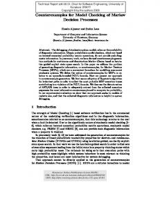
Figure 1: Memory hierarchy for LTL model checking. though hard disks become larger in size, their access behavior hardly scales; with a rotating magnetic disk of 5,400-15,000 rpm mechanical limits become apparent. Flash memory has seen a dramatic increase in power and decrease in price the last few years. High density flash memory cards are available at low prices. The development of solid state disks for substituting hard disks is an apparent consequence. They have no moving parts, and are, therefore, not susceptible to mechanical failure as a result of vibrations. Solid-state disks have a high reliability, and low power consumption. The main argument, however, is that solid-state disks are faster in certain operations like starting an application program and rebooting the computer. Current devices have a burst rate of up to 150 MB/s. Practical data readings of up to 100 MB/s compare well with high-end hard disks. Solid state disks often provide more than 30 MB/s also for writing, the usual backbone of flash memory. The most obvious advantage of solid state disks is the reduced time for random access. The average seek time is often below 0.2 ms, while hard disk seeks often take more than 15 ms. This allows a solid state disk to perform up to 7,000 I/Os per seconds, while a hard disk handles about 60. One observation [3] is that random reads, as needed, e.g. for binary search, are fast, but random writes are not, so that basic operations like external sorting do not obey any speed-up, when invoked on a solid state disk. Due to the discrepancy between random reading and writing, new designs for external-memory algorithms are wanted to exploit the advantages of flash media. Solid state disks will likely not substitute hard disks for large-scale verifications, with terabytes storage requirement [13, ?], for this paper, we assume a three-level hierarchy of: main memory, where data is processed and duplicates are eliminated, solid state disks where compressed states are stored, and hard disks where uncompressed states are kept (Fig. 1). We elaborate on the setting that the future for the verification of software may 2

be found in semi-external model checking [14], which demands a bounded number of bits per state in internal memory. The approach exploits recent advances for the I/O-efficient construction of perfect hash functions [6, 7]. We extend the discussion of semi-external LTL model checking in [14] to find counter-examples of minimal length. We externalize the internal memory-efficient but unimplemented algorithm of Gastin and Moro [16], and include some of its proposed refinements. We establish that finding a minimal counter-example semiexternally shows a good time-space trade-off, close to the non-optimal double depth-first search approach by Edelkamp et al. [14]. Compared to the only other optimal counter-example algorithm of [13], our proposal serves a stronger optimality criterion and has a better worst-case I/O performance. We additionally show that solid state disks can reduce the number of bits per state by moving the hash function from the RAM to the solid state disk. Therefore, we trade the space consumption in RAM (measured in bits) with the I/O complexity on disk (using the standard external-memory model) and the I/O complexity on flash memory (with different I/O-access times for random reads and writes). Let cPFH be the number of bits required (per stored state) to represent the hash function. If the hash function is stored entirely on the flash memory, the RAM requirements for detecting duplicates can be reduced from 1 + cPFH bits per state to 1. The information theoretic lower bound for cPFH is log2 e = 1.442, such that our RAM efficiency is superior to any other compression, which stores the states in main memory. Using only 2 GB RAM, we can enumerate state spaces with up to 231 states. In order to analyze the performance of the algorithms on flash devices, we contribute a complexity model based on linear functions for reading and writing n data elements. It extends the external-memory model of Vitter and Shriver [23] and distinguishes between an offset to access the first data and the efforts for accessing the data in a linear scan. Together with sorting and accessing n elements on disk the new model thus consists of the primitives sort(n), scan(n), write(n), and read(n). The paper is organized as follows. First, we introduce external and semiexternal graph search for reachability and the LTL model checking problem. The algorithms assume a perfect hash function for state vectors. We recall c-bit semiexternal algorithms. We then adapt the recently proposed internal minimal-counter LTL model checking problem to run semi-externally. After introducing the complexity model the approaches are evaluated in the new context of a memory hierarchy that includes flash memory. Afterwards, we provide random data experiments to study the impact of flash memory for semi-external search. 3

2

Algorithms for External and Semi-External LTL Model Checking

Automata-based LTL model checking [8] amounts to detecting accepting cycles in some global state space graph. The first I/O-efficient solution for the LTL model checking problem [13] builds on the reduction of liveness-to-safety property conversion [24] that originally has been designed for symbolic model checking [19]. The algorithm operates on-the-fly and applies heuristics for accelerated LTL property checking [13]. Since the exploration strategy is A* [17], the produced counter-examples are optimal. A further I/O-efficient algorithm for accepting cycle detection [4] is one-waycatch-them-young (OWCTY), which is based on topological sort. The algorithm generates the whole state space and then iteratively prunes away the parts of the state space that do not lead to any accepting cycle. Later on, an external on-thefly LTL model checking algorithm based on the maximal-accepting-predecessors algorithm (MAP) has been developed [5]. The underlying exploration strategy in both cases is a breadth-first enumeration of the state space. To avoid scans of previous layers for duplicate detection especially for large search depths, a delayed merging strategy has been applied. Perfect hashing [6] is a space-efficient way of associating unique identifiers to states. Perfect hash functions yield constant-time random access time in the worstcase. Minimum perfect hash functions are bijective. To construct a minimum perfect hash function for model checking problems, however, it is necessary to generate the entire state space graph first [7]. Practical minimum perfect hash functions [7] can be stored with less than 4 bits per state in RAM. Without insisting on perfect hashing to be minimal, the space performance can be improved slightly. With limited information per state (e.g. one flag for monitoring if a state has been visited), semi-external graph algorithms [1] store a constant number of bits per state. This has motivated the following definition [14]. A graph algorithm A is called c-bit semi-external for c ∈ R+ , if there is a constant c0 > 0, such that for each implicit graph G = (V, E) the internal memory requirements of A are at most c0 ·vmax +c·|V | bits. Including the state vector size vmax in the complexity is necessary, since this value varies for different graphs. Based on this definition, [14] propose semi-external depth-first search with use of minimum perfect hashing. First, an external-memory breadth-first [20] generates all states on disk (hence the semi-external nature). Then, a minimal 4

Perfect hash function, representing 67 states with 5 bits per state.

Visited bit array, representing 67 states with 1 bit per state

Figure 2: State space compression using a perfect hash function.(The position of a visited bit is determined by the states compressed representation in the function) perfect hash function is constructed on the basis of all these states. Finally, the actual verification is performed using this perfect hash function (Fig. 2). For semi-external LTL model checking [14], the double depth-first search algorithm proposed by [9] has been ported from internal to external search. The algorithm performs a first DFS to find all accepting states. The second DFS explores the state space seeded by these states. Besides the amount of storing the perfect hash function, the algorithm requires one additional bit per state. The on-the-fly variant is based on bounded model checking [14]. It is slightly less I/O efficient, but is able to find errors (and the corresponding counter-examples) faster. A strict iterative-deepening strategy searches for counter-examples every time a new BFS level is generated. Since every bounded search applies at most O(sort(|V |)) I/Os, generating the state space for the perfect hash function construction dominates the search complexity. In practice, searching counterexamples was too expensive to be invoked after the completion of each BFS level. Therefore, a check for counter-examples was invoked less frequently while searching on-the-fly.

3

Semi-External Minimal Counterexample LTL Model Checking

Depth-first-search based algorithms (usually) produce non-minimal counter-examples. As we are not aware of an internal linear-time algorithm for finding minimal counter-examples, we cannot expect a number of I/Os linear to the efforts of scanning the search space. Moreover, OWCTY [4] and MAP [5] cannot guarantee minimality of the counter-examples produced. There are two possible criteria for minimal counter-examples (see Figure 3). The external-memory LTL model checking algorithm of [13] produces a minimallength lasso-shaped counter-example τ1 τ2 among the ones that include the accept5

τ2

ρ2 ρ1

τ1

ρ3

Figure 3: Different LTL Counter-Example Optimality Criteria. ing state at the seed state of the cycle. Its worst case I/O complexity is defined by searching the cross product graph with node set |Accept| × |V |. More precisely, the algorithms runs in O(l · scan(|Accept||V |) + sort(|Accept||E|)), where l is the locality of the search graph. The worst-case space consumption amounts O(|Accept||V |), which is large, if |Accept| is large. At least in models with invalid property, due to direct search, the worst-case rarely approaches its worst case. For this paper, we consider an optimality criterion, in which the counterexample is minimal among all lasso-shaped counter-examples ρ1 ρ2 ρ3 not necessarily having an accepting state at the seed of the cycle. It is obvious that the value is smaller than or equal to the above. Here we produce an optimal counter-example with a worst-case I/O complexity, roughly |Accept| times the one of semi-external BFS with internal duplicate detection. As we will see, the algorithm’s I/O complexity amounts to O((l + |Accept|) · scan(|V |) + sort(|E|)), a considerable improvement to [13]. More importantly, the worst-case space consumption is linear in the model size and matches the one of OWCTY [4] and MAP [5]. The following implementation, calling O(|Accept|) semi-external BFS adapts the algorithm of [16]; an internal-memory algorithm that finds optimal counterexamples space-efficiently1 . The algorithm progresses only along forward edges. Figure 4 provides the pseudo-code for the search for a minimal counter-example with solid state and hard disks. The construction of the 1-level bucket based priority queue is shown in Fig.5, while the synchronized traversal is shown in Fig. 6. (The notation is chosen to align with [16], proofs of correctness and optimality are inherited.) The algorithm in [16] consists of three phases, corresponding to the three concatenated sub-paths of the counter-example ρ1 ρ2 ρ3 , path ρ1 to the cycle seed (phase 1), path ρ2 from the seed to the accepting state (phase 3) and path ρ3 back 1

In [16] the algorithm was not implemented. Due to the implementations we found some minor bugs in the pseudo-codes, which, nonetheless, did not harm the correctness proof of the approach.

6

Procedure Minimal-Counter-Example-Search Input: Initial State s, Successor Generating Function succ s : max depth of the BFS starting at s StateSpace : state vectors including BFS level on external memory Accept : accepting state vectors including BFS level on external memory (StateSpace, s ) := External-BFS(s, succ) h : perfect hash function with cPHF × |StateSpace| bits on external memory h := Construct-PHF(StateSpace) visited : internal bit-array [1..|StateSpace|] depth : internal or external array with |StateSpace| × dlog(s + 1)e bits G : file for state vectors on external memory visited := (0..0); G := ∅ (depth, Accept) := BFS-distance(s, succ, G) PQ : internal dynamic array of files for state vectors opt := ∞ for each r ∈ Accept with depth(r) < opt do visited := (0..0); G := ∅ PQ := BFS-PQ(r, succ, G) visited := (0..0); G := ∅ (t, n) := Prio-min(r, succ, PQ, G) if (n < opt) then s1 := t; s2 := r; opt := n visited := (0..0); G := ∅ ρ1 := Bounded-DFS(s, s1 , succ, G, depth(s1 )) visited := (0..0); G := ∅ dist(s1 , s2 ) := BFS(s1 , s2 , succ, G) visited := (0..0); G := ∅ ρ2 := Bounded-DFS(s1 , s2 , succ, G, dist(s1 , s2 )) visited := (0..0); G := ∅ ρ3 := Bounded-DFS(s2 , s1 , succ, G, opt − depth(s1 ) − dist(s1 , s2 )) Figure 4: Semi-External LTL Model Checking Constructing a Minimal CounterExample by traversing the state space with several breath-first-searches.

7

Procedure BFS-PQ Input: Accepting state r, successor generating function succ, file for state vectors G Output: Dynamic array for state vector files on external memory PQ if (depth(r) < opt) then PQ.Append[depth(r)](r) G.Append(r) visited[h(r)] := true n := 0; l := 1; l0 := 0; q := 0; loop := false while (q 6= |G|) and (n < opt)do u := G.Next(); q := q + 1; l := l − 1 for each v ∈ succ(u) do if (visited[h(v)] = false) then visited[h(v)] := true if (depth(v) + n + 1 < opt) then PQ[depth(v) + n + 1].Append(v) G.Append(v); l0 := l0 + 1 loop := loop ∨ (v = r) if (loop) and (depth(v) + n + 1 < opt) then opt := depth(v) + n + 1 if (l = 0) then l := l0 ; l0 := 0; n := n + 1 if (loop) then return PQ else return ∅ Figure 5: Constructing a 1-Level-Bucket Priority Queue of Files.

8

Procedure Prio-min Input: Accepting state r, successor generating function succ, file for state vectors G, dynamic array of state vector files PQ Output: Pair (u, t) of state u and lasso length t n := P min{i | PQ[i] 6= ∅} p := i |PQ[i]|; q := 0; l := 0; l0 := 0 while (p 6= 0 ∨ q 6= |G|) and (n + 1 6= opt) do for each (u ∈ PQ[i] with visited[h(u)]) = false do G.Append(u, u) visited[h(u)] := true p := p − 1; l := l + 1 while l 6= 0 do (u, u0 ) := G.Next() q := q + 2 for each v 0 ∈ succ(u0 ) do if v 0 = r then return (u, n + 1) if (visited[h(v 0 )] = false) then visited[h(v 0 )] = true G.Append(u, v 0 ) l0 := l0 + 1 l := l − 1 l := l0 ; l0 := 0; n := n + 1 return (⊥, ∞)

Figure 6: Synchronized Traversal driven by External 1-Level-Bucket Priority Queue.

9

from the accepting state to the seed (phase 2). Phase 1 of the algorithm executes a plain BFS traversal, that comes for free while constructing the perfect hash function, even though our implementation performs another semi-external BFS for it. This way we could also validate that the perfect hash function works correctly. Phase 2 and phase 3 start a BFS from each accepting state, incrementally improving a bound opt for the minimal counter-example. Phase 3 invokes a BFS driven by an ordering obtained by adding the BFS distances from phases 1 and 2. States in this phase are ordered with respect to |ρ1 | + |ρ3 | and stored in a 1-level bucket priority queue invented by Dial [11]2 . If duplicate elimination is internal, states can be processed in sequence. Hence, all three phases do allow streaming they can be implemented I/O-efficiently. Files are organized in form of queues, but they do not support Dequeue operation, for which deleting and moving the content of the file would be needed. Therefore, instead of Enqueue and Dequeue our algorithms are rewritten based on the operations Append and Next. As a consequence that files do not run empty, and in order to keep the data structures on the external device as simple as possible, we additionally adapted the pseudo code implementation. The counters l and l0 maintain the actual sizes of the currently active and the next BFS layer (at the end of a layer l0 is set to 0 counting the unique successors of the next layer). Value q denotes the current head position in the que file and is incremented after reading an element. When the queue file is scanned completely, all elements are removed and q is set to 0. With constant access time perfect hashing speeds-up all graph traversals to mere scanning. It provides duplicate detection and fast access to the BFS depth (wrt. the initial state) values associated with each state. Finally, solution extraction (slightly different to the one proposed in [16]) reconstructs the three minimal counter-example sub-paths ρ1 , ρ2 , and ρ3 between two given end states using bounded DFS3 . Counter-example reconstruction based on bounded DFS can also be implemented semi-externally. Let opt be the length of the optimal counter-example and dist the length of the shortest path between two states. It is not difficult to see that for start state s, seed state s1 , and accepting state s2 we have |ρ1 | = dist(s, s1 ), |ρ2 | = dist(s1 , s2 ) (to be computed with BFS), and |ρ3 | = opt − dist(s, s1 ) − 2

Originally a heap was used, which is less efficient and does not lead to an elegant externalization. 3 In difference to [16] we avoid overwriting the depth value. The DFS depth is determined by the stack size, such that once the threshold is known, no additional depth information is needed to truncate the search.

10

dist(s1 , s2 ). The reconstruction is slightly different to [16]) as we use the knowledge on |ρ1 | and opt to avoid BFS calls. The implementation already includes performance improvements from [16] while constructing the priority queue. For example, accepting states without loops or over-sized loops are neglected. In experiments, we observed improvements in search time by a factor of about 6. The upper size for the priority queue is bounded by the maximum depth s of the BFS starting at s plus the diameter of the search space diam = maxs1 ,s2 dist(s1 , s2 ). As the latter is not known in advance4 we use dynamic vectors for storing the priority queue. Besides delayed duplicate detection for constructing the perfect hash function, all duplicates are caught in RAM, such that for sorting-based initial external breadth-first search, we arrive at a total hard disk I/O complexity of sort(|E|)+(l+|Accept|+5)·scan(|V |) = O(sort(|E|)+(l+|Accept|)·scan(|V |)).

4

Flash-Based Semi-External LTL Model Checking

Solid state disks are expected to behave like faster hard disks. But sufficiently many differences remain. This implies that advances in external-memory algorithms are needed, even if the basic idea of block transfer will stay. The key idea to improve the RAM-efficiency of semi-external memory algorithms is rather simple. Instead of the hash function being maintained completely in RAM, it is stored (partially or completely) on the solid state disk. The visited bit array that denotes, whether a state was seen before, remains in RAM, consuming one bit per state. Note that static perfect hashing, as approached in this paper, is in contrast to dynamic (perfect) hashing, for which, each time RAM becomes sparse, the foreground function, which is storing the states in the RAM, has to be moved and merged with the background hash function, using external storage, flashefficiently. Most perfect hashing algorithms [15] can be made dynamic [12], but here we have the additional limitation of slow random writes, so that rehashing has to be sequential. In other words, foreground and background hash functions have to be compatible. The design of flash-efficient dynamic hashing algorithms is a research challenge on its own with a large impact for on-the-fly model checking algorithms like nested depth-first search [18]. 4

Only for undirected graphs we have diam ≤ 2 · s .

11

Procedure SSD-LTL-Model-Check StateSpace : State vectors on HDD StateSpace := External-BFS(s, succ) h : Perfect hash function with cPHF × |StateSpace| bits on SSD h := Construct-PHF(StateSpace) visited : internal bit-array [1..|StateSpace|] Semi-External-LTL-Model-Check(s, succ, h, visited)

Figure 7: Flash-efficient semi-external model checking. For our setting we distinguish three phases: state space generation, perfect hash function construction and search. In the construction phase of the perfect hash function for a set of keys, provided as a file, the perfect hash function is constructed, also in form of a file. The external-memory construction process due to [7] is streamed and includes sorting the input data according to some first-level hash function. Therefore, generation can be executed efficiently on the hard disk5 . The extended algorithm with integrated flash memory for storing and accessing the perfect hash function is shown in Fig. 7. It requires one bit per state for early duplicate detection in RAM. For the call to Semi-External-LTL-Model-Check different options are available. For the example of single, or double depth-firstsearch (possibly combined with iterative-deepening) one bit per state in vector visited is sufficient. Exploiting flash memory, the semi-external minimal counter-example algorithms described above can be made 1-bit semi-external, if the BFS depth is attached to the state in the perfect hash function on the solid state disk. Therefore, the number of bits required at each state on solid state disk is enlarged by the logarithm of the maximum BFS layer. Assuming that this value is smaller than 256, one byte per state is sufficient. 5

or from hard disk to solid-state disk or from flash media card to solid state disk. The compression ratio is impressive, e.g., for sets of 10-letter strings, we obtain a 18-fold reduction.

12

Characteristic Volatile Shock Resistant Physical Size Storage Capacity Energy Consumption Price Random Reads Random Writes Sequential Reads Sequential Writes Throughput

RAM Yes Yes Small Small Very High Very Fast Very Fast Very Fast Very Fast Big

Flash Disk No No Yes No Small Large Large Largest Medium High Medium Very Cheap Fast Slow Very Slow Slow Slow Fast Very Slow Fast Smallest Small

Table 1: Rough classification of Flash Media with respect to RAM and Hard Disk

5

Towards a Model for Flash-Efficient Search

For the devices tested in [3], we obtain a qualitative picture as shown in Table 1. For the current progress solid state disk technology the terms for random writes, sequential writes and throughput have already moved towards their disk equivalents. According to the model of Vitter/Shriver [2], for the hard disk I/Os we distinguish between scanning complexity scan(n) = dn/Be and sorting complexity sort(n) = dn/Be logbM/Bc dn/Be, where n is the number of input items that have to be scanned and sorted, B is the number of elements in a block that are accessed in one I/O, and M is main memory capacity (in items). So far, there is no accepted complexity theoretical memory model that covers flash memory. Driven by the observations in [3], we distinguish between writing of n items, denoted as write(n), and reading of n elements, denoted as read(n), mainly because reads are faster than writes. As, according to [3], standard external sorting does not differ much on both media we do not introduce a different term for flash memory. We have to accept that the complexity model we derive is not an exact match. For example there are discontinuities on flash media, e.g. restructuring the access tables requires longer idle times. There is one subtle problem, that we also have to avoid in modeling flash

13

memory, especially when comparing to the disk memory. Most operating systems implicitly use RAM disk 6 . If remaining RAM is available, I/O-intense applications with several reads or writes may not access disk at all, since this may be fully mapped to the RAM. Of course, this approach has limitations, at the time RAM gets exhausted. To avoid side effects we assume direct I/Os, i.e., we bypass all RAM disks. Disk reads also operate block-wise, as reads and writes on hard disk do, so reading small amounts of data from distant random positions takes considerably more time than reading the same amount of data stored linearly. This does match the design of flash media. The difference in read and write on flash devices have to reflect the fact that, since NAND technology is not able to write a single random bit, writing uses block copying and removal, before a small amount of data is written7 . This explains why random writing is significant slower then random reading. As observed by [3], a simple penalty factor is likely to be too pessimistic for random write, as it becomes faster if the data set gets larger. The theoretical model that we suggest is based on linear functions that include both the offsets to prepare the access to the data, and the times for reading it. As hard disk I/Os as well as read and write I/Os differ, we suggest not to count block accesses, but take some abstract notion of time. Nonetheless, we prefer to talk about I/Os. The model we propose distinguishes between the offset (including the seek time and other delays prior to the sequential access), and a linear term for reading the elements. One may either introduce individual block sizes for reading and writing, or devise suitable factors for read and write access. We prefer the second alternative and suggest the following primitives for analyzing algorithms on flash memory: scan(n) = tA + t0A · dn/Be, read(n) = tR + t0R · dn/Be, and write(n) = tW + t0W · dn/Be, where the value • tA denotes the time offset for hard disk access (either for reading or for writing). It reflects the seek time for moving the head to the location of the first data item that is executed only once in a sequential read operation. 6

On modern Unix systems there is even a parameter (swappiness) that controls the operating system in its decision to either swap internal memory to disk or to reduce the RAM disk. 7 The difference between read and write also relates to how the flash memory is organized. Even for NAND devices different trade-offs can be obtained in different designs.

14

• t0A is the time for reaching the next block in a linear scan. • tR and tW are the time offsets for reading and writing data on the flash. With tW being considerably larger than tR this explain the discrepancy between the two operations for random access. • t0R and t0W are the offsets for flash media access per block. Here t0W is only moderately larger than t0R , explaining that the burst rates do not differ that much. As tA is much larger than tR and tW (while t0A is about as large as t0R and t0W ) these terms agree with the observation that for flash media it is less important, where the block is located, while on disk, we clearly prefer blocks that are adjacent. For the actual analysis of an algorithm, we abstract from the values of tA tR , and tW as well as from t0A , t0R and t0W , by deriving complexities wrt. the primitive operations scan(n), sort(n), write(n), and read(n).

6

Analyzing the Algorithm

If the perfect hash function is outsourced to the flash memory, then the semiexternal LTL model algorithm described above improves from being (1 + cPHF )-bit semi-external. We assume RAM to be smaller than flash memory by a factor of more than cPHF . To understand the externalization of the minimum perfect hashing, we briefly motivate its construction process and its usage. Perfect hashing is a one-to-one mapping of some state set V to the index range {0, . . . , |V | − 1}. For the construction of the hash function, the set V has to be known. Perfect hash functions relies on results from random graph theory, that exceeds the scope of the current paper such that we can only outline the basic idea. Space-efficient perfect hashing shares similarities with cuckoo hashing [21] and comprises 2 hash functions and tables8 . The hash functions map elements to the two tables, from which a bipartite graph (see Figure 6) is constructed. An element is either in one table (left) or in the other (right). If we store information, whether or not a state is stored in the left or right hash table the lookup operates is constant time. The crucial observation it that with little extra space in each table, the resulting bipartite graph is acyclic with very high probability. 8

For more than two hash function the results have to be ported to hyper-graph theory.

15

h2 (x)

j

x

h1 (x) i y

m−1

m−1

Figure 8: Bipartite graph based on two hash tables as used for perfect hashing.

For a global state lookup, perfect hashing requires 1 seek, then reading a sequence of bits, depending on the implementation. If the number of bits is smaller than the block size besides multiple calls to the read operation no additional overhead is required. External perfect hashing [7] builds on a partition with buckets of at most n = 256 elements each using a simple first-level hash function, that guarantees 128 bucket elements on the average and no more than 256. For each of the buckets, we now have two individual hash tables on which a bipartite graph is built. The two hash functions of each bucket can be stored compactly in m = 2cn bits, with c ≈ 1.05. If the number of elements in the addressed bucket by a first-level hash function, is 256, then m ≈ 530 bits have to be stored to evaluate the perfect hash function correctly. We implemented two externalizations. In the first one, we only flushed the information on the m bits, which leaves about 184 remaining bits in the RAM. In the second externalization, we flushed all information except the file pointer to the bucket, which reduces the number of bits per bucket to 64. In all our implementations with access to the perfect hash function on flash memory, we store some information of the bucket in RAM, but beat the lower bound of 1.44 bits per state [12]. It is rather simple to extend our implementations to also externalize the remaining bits to the disk9 , such that we can arrive at a 1-bit semi-external algorithm. Such 1-bit semi-external algorithm allows using almost all available RAM for visited bits. The number of hard disk I/Os does not change. For semi-external LTL model checking it is dominated by BFS state space generation. Storing the hash function after generating the state space on hard disk, re9 By using a sparse representation of the buckets. A drawback of writing the uncompressed representation of the buckets on disk is that the file size increase by about 2 (from 128 on the average to 256).

16

quires write(|V |) flash memory I/Os. During (double) depth-first search for each state space edge we pose a query to the hash function, such that O(|E| · read(1)) flash memory I/Os are needed. As the hash function for the on-the-fly variant is computed for each BFS level the flash memory complexity can raise. For minimum counter-example generation we have the following situation. If allocating 1 + cPHF + dlog(s + 1)e bits per node exceed RAM, flash memory can help. Outsourcing the perfect hash function together with the BFS-level takes O(write(|V |)) flash memory I/Os, while total I/O complexity for the the lookups for duplicates detection is bounded by |Accept| · |E| · read(1) flash memory I/Os. Outsourcing the array depth to the solid state disk by enlarging the disk representation of the perfect hash function does not yield additional I/O, as the access to one compressed state with depth value included, is still below the block size. For this case, the access in the pseudo-code would change from depth(v) into depth[h(v)].

7

Experimental Results

For empirical results have consider the following 2 system settings. • ASUS eeeComputer with Intel 900 MHz CPU (32 bit), 512 MB RAM, 4GB on-board solid state disk, with 0.51 ms seek time for one random read and about 23 MB/s for sequential read. From the 4GB SSD about 3 GB were used already for the operating system such that only 1 GB was available for experiments. The computer has an additional SD card slot, which we equipped with a 4 GB SDHC card (1.1 ms random access time, 15 MB/s sequential read) and an external HDD. connected via USB 2.0 (19 ms random access time, 11 MB/s sequential read). • An Desktop PC with AMD Athlon CPU (32 bit) and SATA HDD (Reiser FS) of 280 GB with 13.8 ms seek time and about 61.5 MB/s for sequential reading. We equipped the PC with a 32 GB 3.5” SATA high-speed flash memory solid state disk (HAMA) which has 0.14 ms seek time and about 93 MB/s for sequential reading. We implemented our algorithms in DiVinE (DIstributed VerIficatioN Environment)10 , including only part of the library deployed with DiVinE, namely state 10

http://anna.fi.muni.cz/divine

17

generation and internal storage. For the implementation of external-memory container and for algorithms for efficient sorting and scanning we use STXXL (Standard Template Library for Extra Large Data Sets) [10]. Models are taken from the BEEM library [22].

7.1

Minimal Counter Examples

First, we evaluate the efficiency of the minimum counter-example generation. To save time, we generate the state space on SSD, if possible. We observed a speedup of about 2, compared to the hard disk. Our first case study is Lifts(7) with property P4. The state space consists of 7,496,336 states and 20,080,824 transitions and is generated in 262 layers. Its generation time amounts to about 1122s on the SSD. The perfect hash function is first split into 58 parts, and then finalized in 66s. The first BFS that initialized the depth array, and flushes the set of accepting states, required 187s. The number of accepting states is 2,947,840. Our minimum counter-example algorithm implementation first finds a counter-example with seed depth 81 and lasso length 117 (found within 10s), which is then improved to seed depth 87 and cycle length 2. Proving this to be optimal yields a total run time of 4,035s, with a CPU operating at 86%. According to [14] the non-optimal semi-external double DFS approach takes about 32 minutes to generate one counter-example. Factor 2.1 as a trade-off for optimality is acceptable, as optimality is an assertion about all path, not only about one. For the Szymanski (4) model with property P2, the state space consists of 2,256,741 states and 12,610,593 transitions and is generated in 110 layers. Its generation took 511s on the SSD. The hash function is split into 17 parts. The first BFS took 96s and generated 1,128,317 accepting states. The minimum counterexample length found are 31 = 1 + 30 and 19 = 2 + 11. The last one is optimal. The total run-time is 2,084s. According to [14], semi-external double DFS takes about 10 minutes to generate a counter-example and is thus faster by about factor 3.4 only.

7.2

Flash-Efficient Hashing

In initial experiments, we studied and validated our assumptions about flash media and perfect hash functions. We generated some x million disjoint random

18

strings of length 10, x ∈ {5, 10, 15, 20, 25, 30, 35, 40, 45, 50}11 . From these random strings we generated the perfect hash function using the implementation of Botelho et al. [7] available from the Internet12 . The c-value we took is 4 (for all experiments). The space consumption for the keys are 58 MB, 115 MB, 172 MB, 229 MB, 287 MB, 344 MB, 401 MB. 458 MB, 515 MB, 573 MB, respectively. The perfect hash functions consume 3.8 MB, 6.9 MB, 12 MB, 16 MB, 19 MB, 23 MB, 27 MB, 31 MB, 35 MB, and 38 MB space, respectively. As expected, we observe a good compression. Figure 9 shows that performance in seconds. As the data is still small compared to the RAM, we first observe a influence of OS (in this case Linux) caches in form of RAM disks. Even of the eee Computer all file processing is actually executed in RAM, so that we cannot compare hard to solid state disk performance. This effect cancels out, if we scale space consumption to the limit of RAM, but even then we have to be careful that the operating system does not prefer swapping RAM contents instead of reducing RAM disk size. To measure the efficiency gap between hard and solid state disks, we therefore, enforce direct I/O, and obtain a much fairer picture. These plots are also depicted in Figure 9. As additional effect we see that hard disk performance suddenly drops at about 20 million keys. This is due to the disk cache implemented on the hardware. The ascent is linear, showing that the per-key exploration efficiency stabilizes. These caches can hardly be avoided, they blur the results, but only for small data sets; the effect diminishes for larger data sets. As expected the core reason for the loss in time performance is the amount of I/O wait in the CPU (I/O wait denotes the time the CPU waits for data from external memory). This assertion is validated in Figure 10, showing the percentage of the CPU level for internal processing. We see that RAM disks achieve almost full speed, while the high number of random hard disk reads results in what is denoted as thrashing. We also experimented with 100 and 1,000 million keys on the eee Computer. As the space consumption of 1.2 GB was too much for the remaining amount on the solid state disk, the keys file for perfect hash function creation and for search were read from SDHC card. Even the intermediate file created was stored on SDHC card. The compressed files that store the perfect hash function require 76 11

disjointness is assured by operating system sorting (sort) and duplicate elimination (uniq). The perfect hash generator checks for duplicates, using extra memory, that we avoid. 12 http://cmph.sourcefourge.net

19

200000 eee RAM DISK eee SSD Direct I/O PC SSD Direct I/O PC HDD Direct I/O

180000 160000

time in seconds

140000 120000 100000 80000 60000 40000 20000 0 5

10

15

20

25 30 million keys

35

40

45

50

Figure 9: Time Performance on Random Strings. MB. The CPU time amounts to 30m. for perfect hash function creation. For 1, 000 million keys, the space consumption is 12 GB stored on an external HDD and it takes 5 hours to compute a 757 MB large perfect hash function. Note that the file size for the perfect hash function of 757 MB does not fit into RAM, which is restricted to 512 MB. Moreover, the operating system forbids the solid state disk to serve as swap space. So an implementation that loads the perfect hash function into RAM is infeasible, and an externalization is required. The search for the 100 million keys took 26m, but, unfortunately, the search for 1,000 million keys did not finalize due to hardware failure13 . The RAM consumption were 33 MB and CPU usage was at about 20 %.

7.3

Flash-Efficient Model Checking

Last, but not least we look at the externalization of the hash tables to the SSD. As we have not yet externalized the depth array, we applied LTL model checking with the double DFS implementation of [14]. Table 2 shows our results. First, the space consumption of the data structures for the models is reported, then we 13 The solid state disk stops working properly after running a couple of hours at full speed. We blame the SSD heat, or driver implemetation for this strange behavior.

20

CPU eee RAM Disk CPU eee SSD Direct I/O CPU PC SSD Direct I/O CPU PC HDD Direct I/O

100

80

%

60

40

20

0 5

10

15

20

25 30 million keys

35

40

45

50

Figure 10: CPU Performance on Random Strings. compare the time-space trade-off in three different externalizations. The first one stores the perfect hash function in the RAM, and thus matches the implementation of [14]. The other approaches externalize the hash function via direct I/O on either hard or solid state disk. Note that all experiments have a static storage offset of 238.89 MB due to the inclusion of the Divine model checker and STXXL. Value StateSpace indicates the complexity of each model as stored on the hard disk. We have not used the number of states here to highlight the compression ratio between the size of the statespace and the size of the perfect hash function h. Row h and visited show that the size of h is proportional to the size of the visited array. Since visited is |StateSpace| bits long and h contains a representation of each state this is what one might have expected. Note that the Szymanski protocol needs 4.95 bits per state and the Lifts protocol 6.34 on the average, due to the implementation of Botelho and Ziviani [7] not being capable to create a perfect hash function for this protocol using 4.95 bits per state. For memory comparison between [14] and our extension to it, we report main memory usage for h. The experiments show that the RAM usage drops by a factor of 14 for Szymanski and even by a factor of 20 for the Lifts protocol. As mentioned above, it is possible to externalize h completely, using more space on the external device, without an increase in I/O: the RAM usage is due to the fact 21

Table 2: Flash Performance on Double Depth-First Search on Models with Invalid Temporal Properties (times are given in mm:ss, memory consumption in human readable form). Space Consumption h in RAM h on External Device Experiment StateSpace h visited RAM Time RAM SSD HDD Szyman.(2),P3 1.5MB 38,48KB 7.78KB 28.77KB 0:06 2KB 0:50 0:37 Szyman.(3),P3 65MB 1.33MB 275KB 0.99MB 2:58 68.92KB 39:02 26:11 351MB 5.67MB 915KB 4.55MB 4:27 0.22MB 68:56 48:17 Lifts(7),P4 Lifts(8),P2 1,559MB 25.21MB 4,071KB 20.24MB 19:44 0.99MB 377:22 o.o.t.

that filepointers are stored to every bucket in the h file14 and could be omitted by a constant bucket length in the file. We see that outsourcing h on the external medium needs more time for the search and that for small experiments, where h fits into the hard disk cache, the externalization on hard disk is faster. Lifts(8),P2 is one experiment, where h is larger then 16MB and does not fit into the hard disk cache. The experiment was stopped after six hours of working. During this time the CPU usage never climbed above 5%, while the average CPU usage was 48% on solid state disk. This is exactly the same observation that was made with the random data experiments described above. The time deficiency corresponds to a 19.12 fold slowdown with respect to [14], using 1/20 of the main memory. For very large model sizes [14] is infeasible. Moreover using swap space on solid state disk is prohibited by the operating system, so that hard disk is mandatory as a swapping partition. Time-efficiency is the main argument why to use solid state disk instead of hard disk for storing the perfect hash function in semi-external LTL model checking.

8

Conclusion and Discussion

Recent designs of external-memory algorithms [23] exploit hard disks to work with large data sets that do not fit into RAM, while flash memory devices (solid state disks, memory cards) ask for new time-space trade-offs [3]. Memory cards are cheap, but their access time is limited. In solid state disks (hard disks on flash memory) random reads operate at a speed that lies (in orders of magnitudes) 14

E.g. h(Lifts(8)), is stored in 260,579 buckets (127.99 entries per bucket in average) and a filepointer is 4 byte long which results in 1,042,316B = 0.99MB

22

between RAM and hard disk; while random writes are much slower and should be avoided. Mass production for solid state disks has recently started; in the near future prices are expected to drop and storage capacities are expected to rise. To exploit the advantages of flash memory compared to disk access, semi-external LTL model checking algorithms have been adapted. As random reads are fast, the lesson to be learned is that flash media is good for outsourcing static dictionaries, but generally not for outsourcing dynamic dictionaries that change with random access over time. This restriction in the computational model limits the applicability of flash memory for on-the-fly model checking. Nevertheless, the advent of solidstate disks allows semi-external model checking algorithms to traverse larger state spaces. By exploiting fast random seeks, we obtain interesting trade-offs between loss of speed and savings in RAM. Based on limited time we had for the experiments, we could not scale the model checking problem sizes on the PC hardware, so that the memory requirements for the perfect hash function would exceed main memory. Therefore, we simulated limited RAM by using direct I/O. We have observed that the standard external-memory model by Vitter and Shriver hardly covers the discrepancy between (random) reads and writes. Hence, our refined memory model has been designed for three layers: one for random access, one for flash, and one for the hard disk memory. Basic operations covered by the model are reads and writes on the flash medium and scans and sort to the hard disk. For existing semi-external algorithms, the number of I/Os for accessing the hard disk does not change. Therefore, the design of semi-external algorithms should be the first step for flash-efficient model checking. By externalizing the perfect hash function to the flash, we discussed the transformation of an (1+cPFH )bit to 1-bit semi-external memory algorithms. For minimal counter-example search in LTL model checking, we adapted an internal-memory algorithm to be O(1+cPHF +dlog(s +1)e)-bit semi-external with O((|Accept| + l) · scan(|V |) + sort(|E|)) hard disk I/Os. We discussed a flashefficient solution, which reduces the RAM requirement from (1 + cPHF + dlog s e) bits per state to (1+cPHF ) bits by moving the depth-array to the flash and to 1 bit per state, by additionally moving the perfect hash function to the flash memory. Due to the fact that for minimal counter-example search we perform many independent BFS (one for each accepting state). This suggests an effective parallelization on multi-core processors and on workstation clusters.

23

References [1] J. Abello, A. L. Buchsbaum, and J. Westbrook. A functional approach to external graph algorithms. In ESA ’98: Proceedings of the 6th Annual European Symposium on Algorithms, pages 332–343, London, UK, 1998. Springer-Verlag. [2] A. Aggarwal and J. S. Vitter. The input/output complexity of sorting and related problems. Journal of the ACM, 31(9):1116–1127, 1988. [3] D. Ajwani, I. Malinger, U. Meyer, and S. Toledo. Characterizing the performance of flash memory storage devices and its impact on algorithm design. Technical Report MPI-I-2008-1-001, Max-Planck Institut f¨ur Informatik, Germany, 2008. [4] J. Barnat, L. Brim, and P. Simecek. I/O efficient accepting cycle detection. In CAV, 2007. [5] J. Barnat, L. Brim, P. Simecek, and M. Weber. Revisiting resistance speeds up I/O-efficient LTL model checking. In TACAS, 2008. [6] F. C. Botelho, R. Pagh, and N. Ziviani. Simple and space-efficient minimal perfect hash functions. In F. K. H. A. Dehne, J.-R. Sack, and N. Zeh, editors, WADS, volume 4619 of Lecture Notes in Computer Science, pages 139–150. Springer, 2007. [7] F. C. Botelho and N. Ziviani. External perfect hashing for very large key sets. In CIKM ’07: Proceedings of the sixteenth ACM conference on Conference on information and knowledge management, pages 653–662, New York, NY, USA, 2007. ACM. [8] E. Clarke, O. Grumberg, and D. Peled. Model Checking. MIT Press, 2000. [9] C. Courcoubetis, M. Vardi, P. Wolper, and M. Yannakakis. Memory-efficient algorithms for the verification of temporal properties. Form. Methods Syst. Des., 1(2-3):275–288, 1992. [10] R. Dementiev, L. Kettner, and P. Sanders. STXXL: Standard template library for XXL data sets. In ESA, pages 640–651, 2005. [11] R. B. Dial. Shortest-path forest with topological ordering. Communications of the ACM, 12(11):632–633, 1969. 24

[12] M. Dietzfelbinger, A. Karlin, K. Mehlhorn, F. M. auf der Heide, H. Rohnert, and R. E. Tarjan. Dynamic perfect hashing: Upper and lower bounds. SIAM Journal of Computing, 23:738–761, 1994. [13] S. Edelkamp and S. Jabbar. Large-scale directed model checking LTL. In SPIN, pages 1–18, 2006. [14] S. Edelkamp, P. Sanders, and P. Simecek. Semi-external LTL model checking. In CAV, 2008. [15] M. L. Fredman, J. Koml´os, and E. Szemer´edi. Storing a sparse table with o(1) worst case access time. Journal of the ACM, 3:538–544, 1984. [16] P. Gastin and P. Moro. Minimal counterexample generation in SPIN. In SPIN, pages 24–38, 2006. [17] N. Hart, J. Nilsson, and B. Raphael. A formal basis for the heuristic determination of minimum cost paths. IEEE Transactions on System Science and Cybernetics, 4(2):100–107, 1968. [18] G. J. Holzmann, D. Peled, and M. Yannakakis. On nested depth first search. The SPIN Verification System, pages 23–32, 1972. [19] K. L. McMillan. Symbolic Model Checking. Kluwer Academic Press, 1993. [20] K. Munagala and A. Ranade. I/O-complexity of graph algorithms. In SODA, pages 687–694, 1999. [21] R. Pagh and F. F. Rodler. Cuckoo hashing. In European Symposium on Algorithms (ESA), pages 121–133, 2001. [22] R. Pel´anek. BEEM: benchmarks for explicit model checkers. In SPIN, pages 263–267, 2007. [23] P. Sanders, U. Meyer, and J. F. Sibeyn, editors. Springer, 2003.

Memory Hierarchies.

[24] V. Schuppan and A. Biere. Efficient reduction of finite state model checking to reachability analysis. International Journal on Software Tools for Technology Transfer, 5(2–3):185–204, 2004.

25