Jun 25, 2001 - arXiv:cond-mat/0106494v1 [cond-mat.stat-mech] 25 Jun 2001. Flat histogram simulation of lattice polymer systems. Lik Wee Lee and ...
Flat histogram simulation of lattice polymer systems Lik Wee Lee and Jian-Sheng Wang
arXiv:cond-mat/0106494v1 [cond-mat.stat-mech] 25 Jun 2001
Department of Computational Science, National University of Singapore, Singapore 119260, Republic of Singapore (25 June 2001)
to the broad histogram method [10,11]. However, when it was first proposed by Oliveira et al in 1996, the dynamics gave incorrect results in that the method did not generate true microcanonical averages [6]. When corrected, the flip rate is identical to flat histogram’s but the name remains a historic misnomer. A central quantity in the broad histogram formulation is hN (σ, ∆E)iE , the microcanonical average of the number of potential moves that increase energy by ∆E = E ′ − E. Using this definition together with the requirement that moves must be reversible, a general equation called the broad histogram equation can be derived [12]. Although the definition of hN (σ, ∆E)iE works well for Ising model and can be used to construct the transition matrix T (E → E ′ ), this interpretation is less general and poses a problem for other class of problems, such as polymer system. We shall define a more general quantity, T∞ (E → E ′ ), the transition matrix at infinite temperature or simply called “infinite temperature transition matrix”. The matrix elements of the infinite temperature transition matrix reduces to hN (σ, ∆E)iE for some particular cases. The density of states n(E), corresponds to the left eigenvector of the infinite temperature transition matrix. However, it is easier to obtain the density of states through another set of equations, the detailed balance equations (analogous to the broad histogram equation) explained later. Our procedure for solving the density of states is also different from what is prescribed by the broad histogram method. In the following section, we shall briefly describe our simulation model, the HP model and its connection to protein folding. The subsequent section is on the transition matrix Monte Carlo and flat histogram sampling algorithm. We shall discuss how it can be applied to polymer models. We give some numerical results in the fourth section and the conclusion in fifth section.
We demonstrate the use of a new algorithm called the Flat Histogram sampling algorithm for the simulation of lattice polymer systems. Thermodynamics properties, such as average energy or entropy and other physical quantities such as end-to-end distance or radius of gyration can be easily calculated using this method. Ground-state energy can also be determined. We also explore the accuracy and limitations of this method. 02.70.Uu, 05.10.Ln, 75.40.Mg
I. INTRODUCTION
With the rapid rise of computing power, Monte Carlo methods [1] have become an important tool for studying high-dimensional systems such as proteins, polymers and spin-glass models where many questions remain to be answered. While the Metropolis algorithm [2], due to its simplicity, remains the most popular choice of method, it faces some severe drawbacks. Firstly, the dynamics are slow for a class of problems that involve rugged energy landscapes with multiple local minima. Secondly, a series of simulation at different temperatures is needed to obtain the temperature dependence of thermodynamic quantities. Coupled with slow dynamics, the computation time can be prohibitive. Thirdly, it is difficult to calculate free energy or entropy using this method. While the use of histogram method [3] can alleviate the second problem by reweighting the canonical distribution, the accuracy is limited to a small region in a parameter space. Recent methods based on the direct computation of the density of states are capable of overcoming the abovementioned drawbacks of Metropolis algorithm. The multicanonical method [4] is the earliest of these. Entropic sampling [5] is commonly cited as an equivalent but simpler formulation of multicanonical method. The flat histogram sampling algorithm [6] is able to generate a flat histogram in energy space similar to multicanonical simulations, but in a simpler and more efficient way. The transition matrix Monte Carlo method [7–9] can be used to either obtain the density of states directly or construct the canonical distribution for different temperatures. The method is based upon the definition of a stochastic matrix, the transition matrix T (E → E ′ ). The flat histogram sampling algorithm is an ideal algorithm for obtaining the transition matrix elements through simulations. The transition matrix Monte Carlo method and associated flat histogram sampling algorithm are closely related
II. THE HP MODEL
One of the most challenging problems in computational biology is the problem of protein folding. Proteins are heteropolymer consisting of long chains of amino acids. It is observed that proteins generally adopt a single unique “native” structure. The biological function of a protein is often intimately dependent upon the precise geometrical structure of this folded native state. How does the protein encodes this unique native state in an extremely large conformational space? Understanding this will be a major breakthrough with implications in biochemistry
1
S(σ → σ ′ ) = S(σ ′ → σ). This symmetry in S can be relaxed for general Monte Carlo simulation [17] but is needed for the flat histogram sampling algorithm. By summing up the detailed balance equations for all states σ with energy E and all states σ ′ with energy E ′ , we have X X P (σ)W (σ → σ ′ ) =
and drug design. It is believed that the native state lies at the global free energy minimum. Only a small fraction of the total conformational space can be explored using high-resolution force-field methods. Even more computing power is required when solvent effects are included. Hence coarse grained models have been developed to model the folding process. The HP model [13] is a commonly used simple lattice model with the basic assumption that it is the hydrophobic forces that determines the native structure of the protein. The model recognizes only two types of amino acids: hydrophobic (H) and polar (P). There are some good arguments for supporting this assumption which we shall not elaborate [14]. Our chief concern is to study the statistical mechanical aspect of the model and the performance of our algorithm. Given a sequence of H and P, each self-avoiding chain on a twodimensional lattice is counted as one conformation. Only non-bonded neighbouring HH contributes to the total energy, i.e. ǫHH = −1 and ǫHP = ǫPP = 0. Under such conditions, low-energy conformations are compact with H residues residing mainly in the core and P residues on the outside. The principle disadvantage of this model is that it leads to highly degenerate ground states, especially in three dimensions [15,16].
E(σ)=E E(σ′ )=E ′
X
E(σ)=E E(σ′ )=E ′
E(σ)=E E(σ )=E
we have n(E)f (E)T (E → E ′ ) = n(E ′ )f (E ′ )T (E ′ → E).
(7)
The transition matrix T (E → E ′ ) is also a stochastic matrix with the histogram h(E) = n(E)f (E)/Z being the equilibrium distribution: X h(E)T (E → E ′ ) = h(E ′ ). (8) E
Since the acceptance rate a(σ → σ ′ ) in Eq. (3) is the same for configurations with a fixed energy, T (E → E ′ ) can also be written as a product of two independent factors — the infinite temperature transition matrix T∞ (E → E ′ ) and acceptance rate in energy a(E → E ′ ):
In a Monte Carlo simulation, it is usual to generate a sequence of states {σ 1 , σ 2 , . . .} using a Markov chain where each state denoted by σ lies in the phase space of the model. The Markov chain is defined by a transition matrix W (σ → σ ′ ). This stochastic matrix must satisfy P ′ ′ σ′ W (σ → σ ) = 1 and W (σ → σ ) ≥ 0. In addition, we require the detailed balance condition
T (E → E ′ ) = T∞ (E → E ′ ) a(E → E ′ ),
E 6= E ′ , (9)
where a(E → E ′ ) can be any acceptance rate satisfying Eq. (1), the detailed balance equation, e.g. Metropolis acceptance rate min(1, f (E ′ )/f (E)), and
(1)
to guarantee an equilibrium probability distribution P (σ), i.e. X P (σ)W (σ → σ ′ ) = P (σ ′ ). (2)
T∞ (E → E ′ ) =
X
X
E(σ)=E E(σ′ )=E ′
S(σ → σ ′ ) . n(E)
(10)
When S(σ → σ ′ ) is taken to be a constant, the expression can be simplified. For example, in spin systems we usually pick a spin randomly to be flipped so that S(σ → σ ′ ) = 1/N , for σ and σ ′ related by a single spin flip and zero otherwise, where N is the total number of spins. In this case
σ
It is useful to view the matrix W (σ → σ ′ ) as composed of two independent parts — selection probability S(σ → σ ′ ) and acceptance rate a(σ → σ ′ ). W (σ → σ ′ ) = S(σ → σ ′ )a(σ → σ ′ ).
P (σ ′ )W (σ ′ → σ). (5)
If the configuration probability distribution is a function of energy only, i.e. P (σ) ∝ f (E(σ)), and defining the transition matrix in energy as X X 1 W (σ → σ ′ ), (6) T (E → E ′ ) = n(E) ′ ′
III. TRANSITION MATRIX MONTE CARLO AND FLAT HISTOGRAM SAMPLING METHOD
P (σ)W (σ → σ ′ ) = P (σ ′ )W (σ ′ → σ)
X
(3) T∞ (E → E ′ ) =
For example, the standard Metropolis algorithm [2] uses � � P (σ ′ ) ′ a(σ → σ ) = min 1, , σ 6= σ ′ , (4) P (σ)
X N (σ, ∆E) hN (σ, ∆E)iE 1 = , n(E) N N E(σ)=E
(11) where ∆E = E ′ − E and N (σ, ∆E) represents the number of spins that changes the energy of the current configuration σ by ∆E when flipped, i.e. N (σ, ∆E)/N = P ′ ′ ′ E(σ )=E S(σ → σ ).
′
with S(σ → σ ) usually set to a constant. We can easily check that it satisfies the detailed balance condition when the selection probability S is symmetric, i.e. 2
Substituting the Eq. (9) into Eq. (7), and using the equation f (E) a(E → E ′ ) = f (E ′ ) a(E ′ → E),
(12) FIG. 1. Three types of moves, i.e. crankshaft move.
which is derived from the detailed balance equation Eq. (1) and Eq. (3) with the requirement that S(σ → σ ′ ) is symmetric, which also implies that moves must be reversible, we obtained a set of equations
end, corner and
(17)
To model protein folding by a Markov process, it is necessary to first define the move set. There are several choices and it has been shown that different move sets can affect kinetic quantities, like the mean first passage time [19]. We use a local move set consisting of end, corner and the crankshaft move [20,21]. These are shown in Fig. 1. Note that the end moves are restricted to 90◦ rotations and thus can have one or two possible positions depending on current configuration. The set of valid moves from current conformation σ to new conformation σ ′ is those that can be performed using end, corner or crankshaft move, while preserving the excluded volume constraint. The choice of the move set used will affect the sampling space of configurations and also the correlation time of our algorithm. It can be shown that our set of local moves is non-ergodic, meaning that it does not generate all possible self-avoiding chains on the lattice. However, the number of such configurations is probably negligible compared to our sampling error [21]. We can also consider the definition of our model to include only those states accessible by the move set specified. As long as our native state is accessible, there will not be a problem. The ergodicity problem can be overcome by pivot moves [22]. Pivot moves are defined by randomly choosing a monomer as a pivot and rotating or reflecting one segment of the chain with the pivot as origin. However, pivot moves also fills more entry in our transition matrix making it less banded. Moreover, it is also found that pivot moves do not necessary lead to faster dynamics in the simulation [15]. Although some studies only consider conformations as distinct when they are not related by reflection or rotational symmetry, the choice should not matter since they differ by a factor of 8 in counting the number of states. For the special configurations on a straight line, the factor is 4. However, such configurations have the highest energy and are thus almost negligible. While the selection probability is commonly taken to be 1/N in spin systems, we have some freedom in deciding the specific selection probabilities based on different moves in polymer systems. We list three possibilities.
where H(E) = i=1 δE(σi ),E is the cumulative histogram for a given energy, m is the total number of samples generated so far, σ i is the configuration at step i of the simulation and σ ′i are the available configurations that can be reached from σ i in one move. Whenever data is unavailable to compute the acceptance rate, we simply accept the move in order to sample the unexplored states.
• Given a configuration, we can construct a list of all possible valid moves satisfying the excluded volume constraint. Each move is selected with a fixed equal probability. In practice, we assign moves into a list that can contain up to M moves. Since M is the upper bound to maximum possible valid moves available to any configuration, the remaining unassigned moves are considered invalid. A move is picked at
′
′
′
n(E)T∞ (E → E ) = n(E )T∞ (E → E).
(13)
When S(σ → σ ′ ) is fixed to a constant, we can write n(E)hN (σ, ∆E)iE = n(E ′ )hN (σ ′ , −∆E)iE ′ .
(14)
This equation, known as broad histogram equation, was first presented by Oliveira in [11] and by Berg and Hansmann [18]. Their derivation is based on property that moves between configurations are reversible and is somewhat simpler than our arguments above. However, the interpretation of N (σ, ∆E) cannot be applied when the selection probability is not a constant as the definition of N (σ, ∆E) limits it to be an integer. The general definition of T∞ (E → E ′ ) that can be applied to any choice of S(σ → σ ′ ) is given by Eq. (10). Eq. (13) is a general equation with two important assumptions made in our formulation: the probability of every configuration is a function of its energy only and allowable moves between any pair of configurations are selected with the same probability in both directions. The energy detailed balance equation can thus also be written as h(E) T∞ (E → E ′ ) a(E → E ′ ) = h(E ′ ) T∞ (E ′ → E) a(E ′ → E). (15) If we require that the histogram is constant or flat, i.e. h(E) = h(E ′ ), we choose the acceptance rate � � T∞ (E ′ → E) ′ a(E → E ) = min 1, . (16) T∞ (E → E ′ ) This equation was first proposed in [6] and [9]. While equivalent to the entropic sampling [5] acceptance rate min(1, n(E)/n(E ′ )), the simulation procedure is different. We use a cumulative average to construct the acceptance rate during simulation, i.e. m
T∞ (E → E ′ ) ≈
1 X δ i H(E) i=1 E(σ ),E
X
E(σ′i )=E ′
S(σ i → σ ′i ),
Pm
3
simulation. For other choices of selection probability, we will have to calculate S(σ → σ ′ ) explicitly for each move before adding. Once T∞ (E → E ′ ) is sampled, we solve Eq. (13). Since n(E) varies by a huge order of magnitude, we solved for ln n(E) instead. Broad histogram method uses a forward difference scheme of integration. We solve it instead using a least squares method. When multiple simulations are performed, we can view it as an optimization problem taking the variance of sampling data into account [8].
random. If it is valid, we accept the move using the acceptance ratio in Eq. (16). In our simulation, we set M equal to N , the number of monomers. • Given a configuration, we pick a monomer at random. If it is an end monomer, it is able to rotate to two possible positions.1 We select one randomly without considering the excluded volume constraint. If it is not an end monomer, then corner or crankshaft moves are possible. These two moves are mutually exclusive. Once a move is selected, we check the excluded volume constraint. If a move results in moving a monomer into an already occupied position, the move is rejected. Otherwise, we accept the move using the acceptance ratio in Eq. (16). For cases where no moves are possible for the monomer picked, the current configuration is included in the average and the time step is incremented by one. This method of selecting move is used in Ref. [23]. It relies on the fact that in moving to a new configuration using a particular type of move, only the same type of move in reverse can bring it back to the original configuration. Thus, the move set must be chosen with this property to ensure that selection probability is symmetric.
IV. NUMERICAL RESULTS
We present results on a sequence with 14 monomers with the sequence HHHPHPHPPHPHPH. Through enumeration, we found that this sequence have a unique ground state (i.e. 8 possible configurations in our counting) of energy −7. The full density of states is given in Table I.
• We can designate end moves and corner moves as 1monomer move and crankshaft move as 2-monomer move. With probability e.g. 0.2, we choose to perform 1-monomer move; if an end monomer is picked, end moves are selected and corner moves otherwise, in the same manner as above (see footnote). With remaining probability 0.8, pick a monomer from 1 to N − 3, a 2-monomer move is selected if monomers from i to i+3 forms a crankshaft otherwise a move is unsuccessful. This method is used in Ref. [24].
FIG. 2. Native state for the sequence HHHPHPHPPHPHPH.
TABLE I. Density of states for the sequence HHHPHPHPPHPHPH. n ˜ (E) is Monte Carlo results using flat histogram sampling algorithm and n(E) is through enumeration. E 0 -1 -2 -3 -4 -5 -6 -7
For compact configurations, the rejection rate for the second method would be very high. We use the first method, although a large M can also make the method inefficient for compact (thus low-energy) configurations since the number of possible moves is low compared to the value of M . However, this can be overcome if an N-fold way simulation [25] is done. A move is always accepted in the N-fold way and the average lifetime of a configuration is taken into account when averaging. The first method also has the advantage of saving some computations. Since the selection probability is a constant, we can just add a constant (equivalent to counting moves) when calculating T∞ (E → E ′ ) in Eq. (10). The list of moves can also be used in constructing an N-fold way
1
This is different from our case where 180◦ rotations are not allowed. It is necessary for the number of possible moves of each type be unambiguous for this case.
4
n(E) 581340 228416 56344 12472 2432 464 24 8
n ˜ (E) 540416.37 217016.11 55837.55 12666.23 2465.45 485.93 23.66 8
% error 7.04 5.00 0.89 1.56 1.38 4.73 1.42 0
0
−0.1
−0.2
10 10 rel. error
−0.3
−0.4
10 10 10
−0.5
the increasingly deep kinetic traps with decreasing temperature. The flat histogram sampling algorithm is unaffected by this effect with slightly better accuracy for low temperature range. The single histogram method also produces roughly the same degree of accuracy. Here we do not observe the reweighting errors due to the exponential decay of the canonical distribution because the energy spectrum is narrow and thus adequately sampled. The single histogram method works well only in such a situation. The entropy which can be easily calculated from the knowledge of n(E), is shown in Fig. 5. It is difficult to obtain this from Metropolis simulation.
Metropolis algorithm Flat Histogram Single histogram (T=0.75) exact enumeration
0
0
−2
−4
−6
1
−8
0
0.5
0.5
1
1
1.5
Flat Histogram exact enumeration
1.5
T
0.8
FIG. 3. The average energy per monomer against temperature. The insert shows the relative error between using enumerated n(E) and each method.
0.6
−2
s
10
The average energy per monomer and radius of gyration are plotted in Fig. 3 and 4 and are compared with the single histogram method and the Metropolis algorithm. We used 106 Monte Carlo steps for the flat histogram sampling algorithm and each temperature point of Metropolis algorithm and also the single histogram reweighted at T = 0.75. There are about 140 temperature points in the Metropolis simulation, which requires around a 100 times more computing time compared to the flat histogram simulation. 2.2
0
rel. error
−4
10
Rg
−6
10
−8
0
0.5 1
1
0.5 1
1
1.5 1.5
Finding the energy of the native state is also an important task in protein folding. To generate the native states using Metropolis algorithm, the temperature must be low enough so that the canonical distribution covers the low energy range adequately. However, the canonical distri√ bution has width N and low temperature simulation causes the system to be trapped in local minima. Various methods, such as genetic algorithm [26] and methods employing heuristic [27] have been proposed to overcome this problem. Often, an annealing schedule is adopted whereby the temperature is lowered as the simulation progress. There is no standard way and considerable trial-and-error is necessary. The flat histogram sampling algorithm can be used as a method for determining the native state energy. Since the energy barriers no longer exist, we expect a random walk along the energy scale in the ideal case. An advantage is that in most polymer models, the energy range do not increase rapidly with system size. We also do not have to devise any annealing schedule or adjust many parameters. We can therefore use our algorithm for determining the native state energy. Although we cannot attach any physical significance to the time for finding the
−2
0.5
0
0.5
FIG. 5. The average entropy per monomer against temperature. The insert shows the relative error.
10
0
0
T
0
1.4
−4
10
−5
10
10
10
10
2
1.6
rel. error
0.2
Metropolis algorithm Flat Histogram Single histogram (T=0.75) exact enumeration
1.8
−3
0.4
1.5 1.5
T
FIG. 4. The radius of gyration against temperature. The insert shows the relative error between using enumerated n(E) and each method.
The plots indicate that the Metropolis algorithm becomes unreliable below around T = 0.5. This slowing down in dynamics is also found in [23] and attributed to 5
8
native state since the ensemble is non-Boltzmann (multicanonical), it is still useful for analyzing the performance of our algorithm. This native state time τ0 , the time to reach the native state from an unfolded conformation, is shown for four sequences in Table II. We select the first two sequence to have unique native state. The other two sequences were taken from [26].
10
TABLE II. Sequence of HP monomers used in simulation with their lowest energy and native state time averaged from 104 simulations. The last column is the standard deviation of τ0 .
10
Sequence E0 τ0 σ τ0 HPHPPHPPHH -4 339.7 405.7 HHHPHPHPPHPHPH -7 5641.4 6340.4 HPHPPHHPHPPHPHHPPHPH -9 81788.1 85478.5 PPHPPHHPPPPHHPPPPHHPPPPHH -8 196137.9 318722.3
10
τ0 τd τu 7.1 τ0 ∼ N 5.9 τd ∼ N 5.1 τu ∼ N
7
10
6
10
5
10
4
3
10
2
N 10 14 20 25
1
10
0
10
τu 66.8 592.6 2224.3 8418.0
std 60.7 551.5 3612.3 9616.3
count 4272 2615 638 190
τd 167.3 3229.3 13427.8 44214.1
std 208.3 3940.6 13976.7 61316.7
100
We fit the times to find the minimum energy (native) states and the tunnelling times for the four sequences to a power law. The time to find native state follows approximately τ0 ∝ N 7.1 . The “up” and “down” tunnelling time gives the fitted parameter τu ∝ N 5.1 and τd ∝ N 5.9 respectively. This suggests that the algorithm takes increasingly longer time to reach the lowest energy states but moves easily towards the upper energy levels. It reflects our observation that the flat histogram sampling algorithm does not scale very well for longer chains especially when the density of states increase sharply with energy. This also implies that the performance is not ideal for sequences with a unique native ground state. We note that our simulation is non-Markovian and thus the convergence is difficult to analyze. This can lead to detailed balance violation [28]. However, this problem can be alleviated by a two pass simulation. The first pass is the same as before. The second pass uses a fixed flip rate, min (1, n(E)/n(E ′ )), obtained from the first pass.
TABLE III. Tunnelling times, τu and τd for different sequences. E0 -4 -7 -9 -8
10 N
FIG. 6. The points are native state time and tunnelling times obtained from simulation. The straight lines are fits to a power law τ ∝ N p .
The tunnelling time can also be used as a measure of the efficiency of our algorithm. We denote τu , the “up” tunnelling time as the average MCS taken for a state with minimum energy to reach a state with maximum energy while τd , the “down” tunnelling time is for the opposite direction. These are shown in Table III. Unlike spin systems, where the two tunnelling times are the same due to the symmetry in the Hamiltonian, it is faster to tunnel to higher energies than to lower energies. Fig. 6 shows the general behaviour of the native state time and tunnelling times as the size increases. It is usual in disorder systems to average over different random realizations corresponding to different sets of coupling constants or sequences. However, it is recognized that proteins are not random sequences since they fold into unique native states with specific properties. The probability of selecting a sequence with this property from all possible sequences is very small. This leads to the problem of designing sequences with protein-like properties.
N 10 14 20 25
1
count 4271 2615 638 190
V. CONCLUSION
We have shown that the flat histogram sampling algorithm, which was first proposed and implemented for spin systems, can be used for the simulation of lattice polymer systems. We give some measures of its accuracy and also efficiency in terms of thermodynamics properties, native state time and tunnelling times. The current implementation is useful for up to about 20 monomer HP chain. However, we would like to emphasize that the flat histogram sampling algorithm is still vastly superior to Metropolis algorithm, especially in terms of accuracy for low temperature properties. The simulation time is
6
modest as there is no need for simulation at each temperature point. It also has the advantage of easily obtaining the density of states for free energy or entropy calculations. While the algorithm is rather basic, there are improvements to be made such as the extensions and modifications proposed in Ref. [8].
[24] A. Sali, E. I. Shakhnovich and M. Karplus, J. Mol. Biol. 235, 1614 (1994). [25] A. B. Bortz, M. H. Kalos and J. L. Lebowitz, J. Comput. Phys. 17, 10 (1975). [26] R. Unger and J. Moult, J. Mol. Biol. 231, 75 (1993). [27] L. Toma and S. Toma, Protein Sci. 5, 147 (1996). [28] J.-S. Wang and L. W. Lee, Comp. Phys. Commun. 127, 131 (2000).
[1] K. Binder (ed), The Monte Carlo Method in Condensed Matter Physics, Topics in Applied Phys, Vol 71, 2nd ed, (Springer-Verlag, 1995). [2] N. Metropolis, A. W. Rosenbluth, M. N. Rosenbluth, A. H. Teller and E. Teller, J. Chem. Phys. 21, 1087 (1953). [3] A. M. Ferrenberg and R. H. Swendsen, Phys. Rev. Lett. 61, 2635 (1988); A. M. Ferrenberg and R. H. Swendsen, Phys. Rev. Lett. 63, 1195 and 1658 (1989). [4] B. A. Berg and T. Neuhaus, Phys. Lett. B 267, 249 (1991), B. A. Berg and T. Celik, Phys. Rev. Lett. 69, 2292 (1992). [5] J. Lee, Phys. Rev. Lett. 71, 211 (1993). [6] J.-S. Wang, Eur. Phys. J. B 8, 287 (1999). [7] J.-S. Wang, T. K. Tay, and R. H. Swendsen, Phys. Rev. Lett. 82, 476 (1999). [8] J.-S. Wang and R. H. Swendsen, Transition Matrix Monte Carlo Method, preprint (cond-mat/0104418). [9] S.-T. Li, ‘‘The transition matrix Monte Carlo method”, Ph.D. dissertation, Carnegie Mellon University (1999), unpublished. [10] P. M. C. de Oliveira, T. J. P. Penna and H. J. Herrmann, Braz. J. Phys. 26, 677 (1996); P. M. C. de Oliveira, Braz. J. Phys. 30, 195 (2000). [11] P. M. C. de Oliveira, T. J. P Penna and H. J. Herrmann, Eur. Phys. J. B 1, 205 (1998). [12] P. M. C. de Oliveira, Eur. Phys. J. B 6, 111 (1998). [13] K. F. Lau and K. A. Dill, Macromolecules 22, 3986 (1989). [14] K. A. Dill, S. Bromberg, K. Yue, K. M. Fiebig, D. P. Yee, P. D. Thomas and H. S. Chan, Protein Sci. 4, 561 (1995). [15] P. Clote and R. Backofen, Computational Molecular Biology p229-232, (John Wiley, 2000). [16] K. Yue, K. M. Fiebig, P. D. Thomas, H. S. Chan and E. I. Shakhnovich and K. A. Dill, Proc. Natl. Acad. Sci. USA 92, 325 (1995). [17] W. K. Hastings, Biometrika 57, 97 (1970). [18] B. A. Berg and U. H. E. Hansmann, Eur. Phys. J. B 6, 395 (1998). [19] H. S. Chan and K. A. Dill, J. Chem Phys. 99, 2116 (1993) and 100, 9238 (1994). [20] P. H. Verdier and W. H. Stockmayer, J. Chem Phys. 36, 227 (1962). [21] K. Kremer and K. Binder, Comp. Phys. Rept. 7, 259 (1988). [22] N. Madras and A. D. Sokal, J. Stat. Phys. 50, 109 (1988). [23] N. D. Socci and J. N. Onuchic, J. Chem. Phys. 101, 1519 (1994) and 103, 4732 (1995).
7