Box 118, S-221 00 Lund, Sweden ... 21914, CUMULI and the Swedish Research Council for Engineering Sci- ..... PhD thesis, ISBN 91-628-1784-1, Lund.
Flexible Calibration : Minimal Cases for Auto-calibration� Anders Heyden, Kalle Åström Centre for Mathematical Sciences, Lund University Box 118, S-221 00 Lund, Sweden {heyden,kalle}@maths.lth.se
Abstract This paper deals with the concept of auto-calibration, i.e. methods to calibrate a camera on-line. In particular, we deal with minimal conditions on the intrinsic parameters needed to make a Euclidean reconstruction, called flexible calibration. The main theoretical results are that it is only needed to know that one intrinsic parameter is constant. The method is based on an initial projective reconstruction, which is upgraded to a Euclidean one. The number of images needed increases with the complexity of the constraints, but the number of points needed is only the number needed in order to obtain a projective reconstruction. The theoretical results are exemplified in a number of experiments. An algorithm, based on bundle adjustments and a linear initialization method are presented and experiments are performed on both synthetic and real data.
1. Introduction One of the main goals of computer vision is to extract three-dimensional properties from a number of twodimensional perspective images, for an overview see [4]. One such property is the three-dimensional structure of an object seen in several images. This problem is often called the structure and motion problem, since both the structure of the scene and the motion of the camera are obtained. The classical approach, made by photogrammetrists, is to used pre-calibrated cameras. Then it is possible to reconstruct the object and the motion up to an unknown similarity transformation, for an overview see [2]. In contrast to the classical approach, the uncalibrated reconstruction assumes only image feature correspondences and no calibration information. In this case it is only possible to reconstruct the object up to an unknown projective transformation. � This work has been done within then ESPRIT Reactive LTR project 21914, CUMULI and the Swedish Research Council for Engineering Sciences (TFR), project 95-64-222
During the last years there has been an intensive wave of research on the possibility to obtain reconstructions up to an unknown similarity transformation (often called Euclidean reconstructions), without using fully calibrated cameras. In this case it is necessary to have some additional information about either the intrinsic parameters, the extrinsic parameters or the object in order to obtain the desired Euclidean reconstruction. One common situation is when the intrinsic parameters are constant during the whole (or a part) of the image sequence. Auto-calibration from the assumption of constant intrinsic parameters is traditionally known as selfcalibration. This problem leads to the so called Kruppa equations. These equations are highly nonlinear and difficult to solve numerically. Several attempts to solve this problem have been made, see [11, 5]. In [6] the same problem is solved by a global optimization technique, where a lot of smaller optimization problems have to be solved in order to get a starting point for the last optimization. More recent approaches to self-calibration, using more robust methods, can be found in [1] (using the more general Kruppa constraints), [14] (using the so called modulus constraints) and [15] (using the classical formulation with the absolute conic combined with a robust estimation method). During the last years, several attempts have been made to develop auto-calibration techniques under less restrictions on the intrinsic parameters of the camera. The first step in this direction was made in [7] and another approach using the so called modulus constraint in [13], where the selfcalibration method presented in [14] is extended to allowing changing focal length. However, the practical implications of this result is questionable since when the focal length varies, by zooming, the principal point varies also. In [8], for the first time an existence proof for the possibility to do flexible calibration was given, in the case of known skew and aspect ratio. The next step in the development of flexible calibration techniques was to weaken the assumptions further. Simultaneously, it was shown in [9] and [12] that it is sufficient to know the skew. In fact, it was even shown in the former
paper the more general result that it is sufficient to know any one of the intrinsic parameters. Observe that all other intrinsic parameters are unknown and allowed to vary between the different imaging instances. In this, we will generalize the result on flexible calibration to the case of one constant intrinsic parameter. The theoretical results are verified by experiments on both simulated and real data.
2. Problem Formulation The image formation system (the camera) is modeled by the equation 2 3
2
x γf λ 4y 5 = 4 0 0 1 λx = K [ R j
sf f 0
2 3
3
x0 y0 5 [ R j 1
X
?
? Rt ]X = PX
6Y 7 7 Rt ] 6 4Z 5
,
(1)
1 :
Here X = [ X Y Z 1]T denotes object coordinates in extended form and x = [ x y 1]T denotes extended image coordinates. The scale factor λ, called the depth, accounts for perspective effects and (R; t ) represent a rigid transformation of the object, i.e. R denotes a 3 � 3 rotation matrix and t a 3 � 1 translation vector. Finally, the parameters in the calibration matrix, K, represent intrinsic properties of the image formation system: f represents focal length, γ represents the aspect ratio, s represents the skew and (x0 ; y0 ) is called the principal point and is interpreted as the orthogonal projection of the focal point onto the image plane. The parameters in R and t are called extrinsic parameters and the parameters in K are called the intrinsic parameters. In this paper we will deal with sequences of camera matrices, obeying different constraints on the intrinsic parameters. Let
P
= (Pi = Ki [ Ri
j ? Riti ])i=1
;::: ;
m
about: (i) the plane at infinity (3 parameters), (ii) the absolute conic (5 parameters), (iii) the origin and orientation of the Euclidean coordinate system (6 parameters) and (iv) the global scale (1 parameter). The global scale can not be determined because of the speed-scale ambiguity. The origin and orientation of the Euclidean coordinate system are internal Gauge freedoms, i.e. depends on how a coordinate system is chosen. The plane at infinity encodes the affine structure and is represented by its normal vector containing 4 components defined up to scale in the projective space. Finally, the absolute conic encodes the Euclidean structure within the affine space and is represented by a symmetric 3 � 3 matrix defined up to scale. The main goal of the existence proofs that will be presented in this paper is to characterize the set of projective transformations H such that the transformed camera matrices Pi H can be factorized as Pi H � Ki [ Ri j
? Riti ]
;
(3)
where Ki fulfils the desired constraints. We are now ready to state the flexible calibration problems from constant intrinsic parameter more formally: Problem 2.1. (Flexible calibration from constant intrinsic parameter) Given a projective reconstruction of the scene in the form of a sequence of camera matrices, characterize the subset of projective transformations H that makes it possible to factorize Pi H as in (3) with Ki representing an intrinsic calibration matrix with one intrinsic parameter constant. Although this problem formulations seems similar to the problem of flexible calibration from one known intrinsic parameter, see [9] it is of a more complex nature, Moreover, it does not follow from the solution to flexible calibration from known intrinsic parameter that Problem 2.1 is solvable.
(2)
denote a sequence of m camera matrices. We make the following definitions: Definition 2.1. A sequence of camera matrices containing cameras modeled as in (1), with constant s is called a constant skew sequence. When γ is constant it is called an constant aspect-ratio sequence and when both s and γ are constant it is called a rigid image sequence. When a projective reconstruction has been obtained, the camera matrices are known up to an unknown projective transformation, i.e. (Pi ) and (Pi H ) are both valid sequences of camera matrices for any non-singular 4 � 4 matrix H. The projective transformation H contains 15 parameters (16 parameters defined up to scale) encoding information
3. Constraints on the Camera Matrices We start with a lemma giving the constraints for sequences of camera matrices with one constant intrinsic parameter. Lemma 3.1. A sequence of camera matrices (Pi ) with 2
uTi Pi = 4 vTi wTi
3
ti 5
;
(4)
normalized such that wi :wi = 1, represents a constant skew sequence, a constant aspect ratio sequence, a camera with constant focal length, a camera with constant x-coordinate
and y-coordinate of the principal point if and only if
� wi ) (vi � wi) jvi � wi j2 j(ui � wi) � (vi � wi )j j(vi � wi )j2 jvi � wi j (ui
:
(5) (6)
ui :wi
(7) (8)
vi :wi
(9)
respectively is constant. Proof. Insert the notations above in (1) and manipulate then the equations 8 T u = γ f r1 + s f r2 + x0 r3 ; >
: T w = r3
cameras with constant focal length, constant x-coordinate of principal point and and constant y-coordinate of principal point, respectively. Note that the sequences of camera matrices with, e.g. s = s0 form a sub-manifold of MScs , des=s s=s0 will noted MScs 0 , etc. In particular, an element in MScs 0 be denoted by (Pi )s=s , etc. The subclass of transformations that preserves the properties in Lemma 3.1 is denoted by GScs , GSca , GSc f , GScx and GScy respectively. Again the group of similarity transformations is contained in GScs , GSca , GSc f , GScx and GScy since these transformations do not change the intrinsic parameters. Theorem 4.1. Let GScs , GSca , GSc f , GScx and GScy respectively denote the class of transformations in 3D-space that preserves the conditions in Lemma 3.1 and GS the group of similarity transformations in 3D-space. Then
(10)
GScs = GSca = GSc f
:
= GScx = GScy = GS 0
4. Proof of Minimal Conditions For a moment, we do not take into account the special form of the camera matrices, (1), for cameras with a constant intrinsic parameter, and instead work with totally uncalibrated cameras. Then it is possible to make reconstruction up to an unknown projective transformation. This means that it is possible to calculate camera matrices Pi , i = 1; : : : ; m that fulfills i = 1; : : : ; m
(11)
:
Given one sequence of camera matrices, Pi , i = 1; : : : ; m, and a reconstruction, X, also Pi H, i = 1; : : : ; m and H ?1 X is a possible choice of camera matrices and reconstruction, where H denotes a non-singular 4 � 4 matrix. The goal is to characterize the set of projective transformations H such that the transformed camera matrices Pi H can be factorized as Pi H � Ki [ Ri j ? Riti ], where Pi H fulfils the corresponding constraint in Lemma 3.1. Let MSP denote the manifold of all (possibly infinite) sequences of camera matrices. The group consisting of all projective transformations, i.e. GP acts on the manifold MSP in the following way ?
f=f0
�
GP � MSP 3 H ; (Pi )
,
y = x = and MScy0 are fixed under transformations with MScx0 elements in GS , implying that it is not possible to transform x00
λi xi = Pi X;
γ=
:
s=s , M Moreover, the sub-manifolds MScs Scg , MSc f γ0
7! (PiH ) 2 MSP
:
In the same way the group GS of similarity transformation acts on the manifold MSP . Denote by MScs , MSca , MSc f , MScx and MScy the submanifold of all sequences of camera matrices that represents constant skew cameras, constant aspect-ratio cameras,
y00
between two different values of the constant intrinsic parameter. Proof. From the discussion above we have GS � GS�� , where again �� is one of the properties in Lemma 3.1. Assume that we have a sequence of camera matrices, (Pi ) 2 MS�� , with Pi = Ki [ Ri j ? Ri ti ]. We may without restrictions assume that s = 0, γ = 1, f = 1, x0 = 0 or y0 = 0 in Ki , since changes of coordinate systems in the images achieves this. Now, we would like to characterize the set of transformations, H, such that H (Pi ) 2 MS�� . Let �� denote one of the cases: s = s0 , γ = γ0 , f = f 0 , x0 = x00 or y0 = y00 , with s0 6= 0, γ0 6= 1, f0 6= 1, x00 6= 0 and y00 6= 0 and let � denote one of the cases: s = 0, γ = 1, f = 1, x0 = 0 or y0 = 0. Assume that H (Pi ) 2 MS�� �� , We now have Pi = Ki� [ Ri j ? Riti ] and HPi � Ki�� [ R0i j ? R0iti0 ]. Combining these equations gives Ki� [ Ri j ti ]
�
Ab c d
�
�
= Ki [ Ri A + ti c
j Ri b + tid ] � K¯i��[ R0i j ti0 ]
Choosing ti = 0 gives Ki� Ri A � K¯ i�� R00i . Assume that A has the property that for every sequence of calibration matrices Ki� and orthogonal Ri , it is possible to factorize Ki� Ri A according to Ki� Ri A � K¯ i�� R00i , for some sequence of calibration matrices K¯ i�� and orthogonal R00i . Then also UAV has this property for every pair of orthogonal matrices U and V . Thus we might replace A with D1 = UAV = diag(a; b; c), where a, b and c denote the singular values of A. Thus we 00 get Ki� R00i D1 � K¯ i�� R000 i and choosing Ri = I we obtain Ki� D1 � K¯ i�� R000 i
:
(12)
:
The left hand side of (12) is upper triangular implying that R000 i = I. Constant aspect-ratio: Writing out (12) gives 2
af 40 0
3
2
ax0 γ0 f 0 5 4 by0 � 0 0 c
as f bf 0
s0 f f0 0
3
x00 y00 5 1
(13)
implying (a f )=(b f ) = (γ0 f 0 )( f 0 ) and a = γ0 b. Making a permutation of a and b gives b = γ0 a, from which it follows that γ0 = 1. Constant skew: Writing out (12) in this case gives 2
aγ f 4 0 0
3
2
ax0 γ0 f 0 by0 5 � 4 0 c 0
0 bf 0
s0 f f0 0
3
x00 y00 5 1
(14)
5. Finding a Solution using Bundle Adjustments
(15)
A bundle adjustment algorithm was developed for estimating all unknown parameters, from an initial estimate. The motivation for this algorithm is as follows. Introduce parameters for all 3D-points, X j , all unknown intrinsic parameters in Ki , all rotation matrices Ri and all translation vectors ti , as in (1). Given these parameters, calculate the coordinates of the resulting image points xˆi; j (image number i and point number j) from (1),
implying s0 f = 0 and thus s0 = 0. Constant focal length: Writing out (12) again gives 2
3
2
aγ as ax0 γ0 f 0 40 5 4 b by0 � 0 0 0 c 0
3
s0 f f0 0
x00 y00 5 1
implying b= f 0 = c and b = f 0 c. Making a permutation of b and c gives c = f 0 b, from which it follows that f 0 = 1. Constant x0 or y0 : Writing out (12) gives immediately x00 = 0 and y0 = 0 similarly to the case of constant skew. In all cases we have reduced property �� to property �, i.e. we know that γ0 = 1, s0 = 0, f 0 = 1, x00 = 0 or y00 respectively. From the theorem on flexible calibration from one known intrinsic parameter, see [9], it follows immediately that GS�� � GS and the theorem is proven. This theorem is valid only under the assumption that the camera motion is sufficiently general and that an infinite number of images covering all possible choices of Ki , Ri and ti are available. This fact is used implicit in the formulation of the theorem and in the proof, by requiring that Pi = Ki [ Ri j ? Riti ] can be chosen arbitrarily. However, it can be argued that only a finite number of images are needed in order to auto-calibrate the camera. The only requirement is that the camera motion has to be sufficiently general. Start with a projective reconstruction represented by a sequence of camera matrices (Pi ), with P1 � [ I j 0 ]. Then the projective transformation H is of the form 2
γf 60 H =6 40 a
sf f 0 b
x0 y0 1 c
3
0 07 7 05 1
;
at infinity (in total 8 parameters). The sequence of transformed camera matrices (Pi H ) has to obey one of the constraints in Lemma 3.1. Assuming that only one intrinsic parameter is constant, we obtain one polynomial constraint for each camera (apart from the first one). Thus at least 10 images are needed to obtain a unique solution (9 equations in 8 unknowns), i.e. one more image than in the case of a known intrinsic parameter. In the case of rigid image planes we have 2 polynomial constraints from each image (apart from the first one), requiring at least 6 images to obtain a unique solution, i.e. 2 more than in the case of Euclidean image planes.
(16)
containing the unknown intrinsic parameters of the first camera and parameters describing the location of the plane
xˆi; j = f (Ki ; Ri ; ti ; X j )
(17)
:
The goal of the bundle adjustment algorithm is to minimize the deviation of these re-projected coordinates to the actual measured coordinates in the 2-norm, i.e.
∑(xi j ? xˆi j )2
min
Ki ;Ri ;ti ;X j i; j
;
;
(18)
:
This solution is actually optimal in a statistical sense, i.e. when the measured coordinates of the image points are assumed to be corrupted by Gaussian noise of zero mean and equal standard deviation. In fact, it can be proven that the Cramér-Rao lower bound is reached, see [10, 3]. In general, the Gauss-Newton method is used to find the minimum, see [2]. Other variants of this methods can also be found, e.g. Levenberg-Marquardt, see [6]. Let m denote the number of images and n the number of points. Denote by m the bundle of all unknown parameters, m = fP1 ; : : : ; Pm ; X1 ; : : : ; Xn g. Each such element belongs to a non-linear manifold, M . Introduce a local parameterization m(∆x), around m0 2 M according to
M
� RN 3 (m0 ∆x) 7! m(m0 ∆x) 2 M ;
;
;
(19)
where N = 10m + 3n + 1 if one intrinsic parameter is constant. For convenience the local parameter ∆x is divided into two parts according to ∆x = [ ∆a1 ; : : : ; ∆am ; ∆b1 ; : : : ; ∆bn ]T , i.e. ∆ai parameterize
changes in camera matrix Pi and ∆b j parameterize changes in reconstructed point X j . Each camera matrix is written Pi = Ki [ Ri j ? Riti ] and changes in Ki are parameterized as fi (m0 ; ∆x) = f + ∆ai (1) etc., where the ∆ai :s are restricted differently according to the different assumptions on the intrinsic parameters. Changes in Ri are parameterized as Ri (m0 ; ∆x) = exp([ ∆ai (6) ∆ai (7) ∆ai (8) ]�)Ri and changes in ti and X j similarly (using ∆b j for X j ). Introduce a residual vector Y, formed by putting all deviations between measured and re-projected image coordinates in a column vector. These residuals depend on the measured image positions xi j as well as on the estimated parameters m. The sum of squared residuals f = YT Y is minimized with respect to the unknown parameters ∆x, using the Gauss-Newton method as follows. A linearization of Y(∆x) gives Y(∆x) � Y(0) +
∂Y (0) ∆x ∂∆x
(20)
:
We want to find ∆x so that Y(∆x) = 0, giving the update ∆x = ?(AT A)?1 AT b;
A=
∂Y (0); b = Y(0) ∂∆x
;
(21)
In practice it is useful to use the Levenberg-Marquardt method, i.e. to add εI to AT A before taking the inverse, where ε is a small positive number. A method to find initial values, proposed by Pollefeys in [12], is based on (16), originating from [7], [1]. This method is based on the assumptions that, generally, the principal point, skew and aspect ratio can be guessed fairly accurately, e.g. s = 1, γ = 1, and principal point located in the centre of the image. Starting from (3), inserting (16) and eliminating Ri by multiplying with the transpose gives (considering the first 3 � 3 block) K1 K1T
�
�
PiT
K1 K1T nK1T
�
K1 nT Pi nnT
:
(22)
and adding the assumptions made above on the intrinsic parameters This equations contains 6 linear equations in the 7 unknowns λi , λi fi , fi , a, b, c and a2 + b2 + c2 . Thus we can solve for n and fi using a quasi-linear method, when at least three images are available.
6. Experiments Experiments have been performed on both simulated and real data in order to show the applicability of the presented flexible calibration techniques and to compare the different constraints to each-other. Simulated data: An experiment was performed with 27 points in 26 images. The points were positioned regularly with coordinates between ?500 and +500 units. The
−3
1.5
x 10
1
0.5
0
−0.5
−1
−1.5
−2
0
5
10
15
20
25
30
Figure 1. The estimated skew for aspect free cameras (solid curve), constant aspect ratio (dashed curve), rigid image planes (solid horizontal line) and constant skew (dotted horizontal line).
camera positions were chosen at random approximately 1000 units away. Also the orientation were chosen at random. The intrinsic parameters were chosen as follows: f = 1000 + N (0; 50), s = 0, γ = 1, (x0 ; y0 ) = (0; 0) + (N (0; 10); N (0; 10)), where N (0; σ) denotes a stochastic variable with mean zero and standard deviation σ. The magnitude of the calculated image coordinates are approximatively 500 pixels. Finally, a stochastic error of standard deviation 1 pixel has been added to the image coordinates. Experiments have been performed on these simulated data by starting close to the simulated values of the structure and motion and applying the bundle adjustment algorithm in the cases Euclidean image planes (s = 0, γ = 1), non-skew cameras (s = 0), aspect-free cameras (γ = 1), rigid image planes, constant skew cameras and constant aspect ratio cameras. In Figure 1 the obtained skew in each camera is plotted. In Table 1 the RMS (root mean square) of the errors are shown in all six cases. Note that the RMS in the images, i.e. the error between the re-projected and the given image coordinates, decreases when more parameters are allowed to vary, but are similar for known and constant parameters. Note also that the estimates of the aspect ratio and skew are very accurate, especially when they are assumed to be constant. Moreover, the errors in focal length are rather small compared to the variation of the focal length and the error in the principal point is only a few pixels. Real data: We have tested the algorithms on real image data. Figure 2 shows one of 42 images of a scene containing point markers and some curves and silhouettes. The images have been taken by the same camera without zooming or focusing. Firstly a projective reconstruction was made using iterative factorization followed by projective bundle adjustment. Secondly, Pollefeys method was used to calculate initial Euclidean structure and motion assuming known
Eip ns af rip cs ca
∆f 1.735 1.964 2.002 1.709 2.168 2.711
image 0.891 0.878 0.880 0.891 0.878 0.880
∆γ n.a. 8.805 n.a. 0.000 8.960 0.000 �10?4
∆s n.a. n.a. 7.723 0.000 0.000 8.378 �10?4
∆x0 1.534 2.040 2.155 1.490 2.136 2.906
∆y0 1.478 2.214 1.663 1.506 2.412 2.094
References
Table 1. Root mean square errors of the reprojected coordinates and the estimated intrinsic parameters for Euclidean image planes (Eip), nonskew cameras (ns), aspect-free cameras (af), rigid image planes (rip), constant skew cameras (cs) and constant aspect ratio cameras (ca). 120
100
80
60
40
20
0 −4
−3
−2
−1
0
1
2
3
4
5
500
f1
450
f2
400
350
300
x0
250
200
150
y0 100
50
0
0
5
10
15
20
25
30
sic parameter or even from the knowledge that only one intrinsic parameter is constant, called flexible calibration. We have also presented an algorithm that auto-calibrate the camera from these assumptions and shown the applicability on both real and simulated data.
35
40
Figure 2. One of 42 images used in the experiment. Histogram of re-projected residuals. Estimated focal lengths and principal point coordinates for the 42 images.
skew, aspect ratio and principal point. This result was then used as initial values to the bundle adjustment routine in the case of non-skew cameras. In Figure 2 is also shown a histogram of errors between estimated point positions and re-projected point positions. In the same figure are shown the two focal lengths ( fx and fy ) and the coordinates of the principal point (x0 and y0 ) for the image sequence. Note that the magnitude of the errors is a few pixels and that the focal lengths and the coordinates of the principal point are in reality constant.
7. Conclusions In this paper we have shown that it is possible to autocalibrate a camera from the knowledge of only one intrin-
[1] K. Åström and A. Heyden. Euclidean reconstruction from constant intrinsic parameters. In Proc. International Conference on Pattern Recognition, Vienna, Austria, pages 339– 343, 1996. [2] K. B. Atkinson. Close Range Photogrammetry and Machine Vision. Whittles Publishing, 1996. [3] H. Cramér. Mathematical Methods of Statistics. Princeton University Press, 1946. [4] O. Faugeras. Three-Dimensional Computer Vision. MIT Press, Cambridge, Mass, 1993. [5] O. D. Faugeras, Q.-T. Luong, and S. J. Maybank. Camera self-calibration: Theory and experiments. In G. Sandini, editor, ECCV’92, volume 588 of Lecture notes in Computer Science, pages 321–334. Springer-Verlag, 1992. [6] R. I. Hartley. Euclidean reconstruction from uncalibrated views. In J. L. Mundy, A. Zisserman, and D. Forsyth, editors, Applications of Invariance in Computer Vision, volume 825 of Lecture notes in Computer Science, pages 237–256. Springer-Verlag, 1994. [7] A. Heyden. Geometry and Algebra of Multiple Projective Transformations. PhD thesis, ISBN 91-628-1784-1, Lund University, Sweden, 1995. [8] A. Heyden and K. Åström. Euclidean reconstruction from image sequences with varying and unknown focal length and principal point. In Proc. Conf. Computer Vision and Pattern Recognition, pages 438–443, 1997. [9] A. Heyden and K. Åström. Minimal conditions on intrinsic parameters for Euclidean reconstruction. In Proc. 22nd Asian Conf. on Computer Vision, Hong Kong, China, 1998. [10] K. Kanatani. Statistical Optimization for Geometric Computation: Theory and Practice. Elsevier Science, 1996. [11] Q.-T. Luong. Matrice Fondamentale et Calibration Visuelle sur l’Environnement-Vers une plus grande autonomie des systèmes robotiques. PhD thesis, Université de Paris-Sud, Centre d’Orsay, 1992. [12] M. Pollefeys, R. Koch, and L. Van Gool. Self-calibration and metric reconstruction in spite of varying and unknown internal camera parameters. In Proc. 6th Int. Conf. on Computer Vision, Mumbai, India, 1998. [13] M. Pollefeys, L. Van Gool, and A. Oosterlinck. Euclidean reconstruction from image sequences with variable focal length. In B. Buxton and R. Cipolla, editors, ECCV’96, volume 1064 of Lecture notes in Computer Science, pages 31–44. Springer-Verlag, 1996. [14] M. Pollefeys, L. Van Gool, and M. Oosterlinck. The modulus constraint: A new constraint for self-calibration. In Proc. International Conference on Pattern Recognition, Vienna, Austria, pages 349–353, 1996. [15] B. Triggs. Autocalibration and the absolute quadric. In Proc. Conf. Computer Vision and Pattern Recognition, 1997.