Jan 28, 2013 - performance, high fidelity multiscale biomedical simulations .... submodel requires a local machine with a set of Python libraries, and another ..... with a voxel size of 3.5Ã10â5 m and consisting of about 4.2 million lattice sites.
arXiv:1211.2963v2 [cs.DC] 28 Jan 2013
Flexible composition and execution of high performance, high fidelity multiscale biomedical simulations D. Groen1 , J. Borgdorff2 , C. Bona-Casas2 , J. Hetherington1 , R.W. Nash1 , S.J. Zasada1 , I. Saverchenko3 , M. Mamonski4 , K. Kurowski4 , M.O. Bernabeu1 , A.G. Hoekstra2 & P.V. Coveney1 1 2
Centre for Computational Science, University College London, UK.
Section Computational Science, University of Amsterdam, the Netherlands 3 4
Leibniz-Rechenzentrum, Garching, Germany
Poznan Supercomputing and Networking Center, Poznan, Poland
Abstract Multiscale simulations are essential in the biomedical domain to accurately model human physiology. We present a modular approach for designing, constructing and executing multiscale simulations on a wide range of resources, from desktops to petascale supercomputers, including combinations of these. Our work features two multiscale applications, instent restenosis and cerebrovascular bloodflow, which combine multiple existing single-scale applications to create a multiscale simulation. These applications can be efficiently coupled, deployed and executed on computers up to the largest (peta) scale, incurring a coupling overhead of 1 to 10% of the total execution time.
1
Introduction
Models of biomedical systems are inherently complex; properties on small time and length scales, such as the molecular or genome level, can make a substantial difference to the properties observed on much larger scales, such as the organ, full-body and even the population level; and vice-versa [1, 2]. We therefore need to apply multiscale approaches when modelling many biomedical problems. Example biomedical multiscale challenges include predicting the impact of a surgical procedure [3], investigating the effects of pathologies (e.g. arterial malformations or fistulas [4]), or assessing the effects of a targeted drug on a given patient [5]. In all these cases, we need to examine processes that not only occur across several time and/or length scales, but that also rely on different underlying physical and/or biological mechanisms. As a result, modelling these
1
processes may require substantially different algorithms and varying levels of computational effort. Historically, these problems have often been modelled using single scale approaches, focussing exclusively on those aspects of the problem which are deemed most relevant. However, applying a single scale model is frequently insufficient to fully understand the problem at hand, as additional processes occurring on different scales must be incorporated to obtain sufficient accuracy. It is this need for understanding the composite problem, rather than its individual subcomponents alone, that has driven many research groups to explore multiscale modelling; for example [6, 7, 8, 9]. In a multiscale model, the overall system is approximated by coupling two or more single scale submodels. Establishing and performing the data exchange between these submodels is an important aspect of enabling multiscale modelling. It is often addressed by using coupling tools, such as MUSCLE [10, 11], the Multilevel Communicating Interface [12] and GridSpace [13]. Groen et al. [14] provide a review of coupling tools and the computational challenges they address. Another important aspect is adopting a data standard which submodels can adopt to exchange meaningful quantities. Several markup languages, such as SBML [15] and CellML [16], resolve this problem by providing a description language for the storage and exchange of model data and submodel definitions. CellML specifically allows for submodel exchange between ODE and PDE solvers, whereas SBML is aimed towards biochemical pathway and reaction ODE submodels. Both SBML and CellML, being languages for the description of submodels and system data, have serious limitations in that they require additional tools to perform tasks that are not directly related to ensuring data interoperability. These include transferring data between submodels, deploying submodels on appropriate resources and orchestrating the interplay of submodels in a multiscale simulation. Additionally, they only provide very limited features to describe submodels that do not rely on ODE-based methods, such as finite-element/volume methods, spectral methods, lattice-Boltzmann, molecular dynamics and particle-based methods, which are of increasing importance in the biomedical domain. Here we present a comprehensive approach to enable multiscale biomedical modelling from problem definition through the bridging of length and time scales, to the deployment and execution of these models as multiscale simulations. Our approach, which has been developed within the MAPPER project 1 , relies on coupling existing submodels and supports the use of resources ranging from a local laptop to large international supercomputing infrastructures, and distributed combinations of these. We present our approach for describing multiscale biomedical models in section 2 and for constructing and executing multiscale simulations on large computing infrastructures in section 3. We describe our approach for biomedical applications in section 4. We have applied our approach to two biomedical multiscale applications, in-stent restenosis and 1 http://www.mapper-project.eu/
2
hierarchical cerebrovascular blood flow, which we present in sections 5 and 6 respectively. We conclude with a brief discussion.
2
Multiscale biomedical modelling
Multiscale modelling gives rise to a number of challenges which extend beyond the translation of model and system data. Most importantly, we seek to allow application developers, such as computational biologists and biomedics, to couple multiscale models for large problems, supporting any type of coupling, using any type of submodel they wish to include, and executing this using any type of computational resource, from laptop to petascale. Since we cannot expect computational biologists to have expertise in all the technical details of multiscale computing, we also aim to present a uniform and easy-to-use interface which retains the power of the underlying technology. This also enables users with less technical expertise to execute previously constructed multiscale simulations. Multiscale systems are, in general, characterized by the interaction of phenomena on different scales, but the details vary for different scientific domains. To preserve the generality of our approach, we adopt the Multiscale Modelling and Simulation Framework (MMSF) to reason about multiscale models in a domain-independent context and to create recipes for constructing multiscale simulations independent of the underlying implementations or computer architectures. This MMSF is based on earlier work on coupled cellular automata and agent-based systems [17, 18] and has been applied to several computational problems in biomedicine [19, 20, 3]. Within the MMSF, the interactions between single-scale submodels are confined to well-defined couplings. The submodels can therefore be studied as independent models with dependent incoming and outgoing links. The graph of all submodels and couplings, the coupling topology, can either be cyclic or acyclic [21]. In a cyclic coupling topology the submodels will exchange information in an iterative loop, whereas in an acyclic topology the submodels are activated one after another, resulting in a directional data flow which makes them well-suited for workflow managers. Two parts of the MMSF are particularly useful for our purposes, namely the Scale Separation Map [17] and the Multiscale Modelling Language (MML) [22, 11]. The Scale Separation Map is a graphical representation which provides direct insights into the coupling characteristics of the multiscale application. MML provides a formalization of the coupling between the submodels, independent of the underlying implementation. In addition, it simplifies the issues associated with orchestrating submodels by capturing the orchestration mechanisms in a simple model which consists of only four distinct operators. MML definitions can be stored for later use using an XML-based file format (xMML) or represented visually using graphical MML (gMML) [11]. The generic MML definitions allow us to identify commonalities between multiscale applications in different scientific domains. Additionally, the stored xMML can be used as input for a range of supporting tools that facilitate multiscale simulations (e.g., tools that automate the deployment or the submodel
3
coupling of these simulations, as discussed in section 3).
3
From multiscale model to production simulation
We have developed a range of tools that allow us to create, deploy and run multiscale simulations based on the xMML specification of a multiscale model. Two of the main challenges in realising successful multiscale simulations are to establish a fast and flexible coupling between submodels and to deploy and execute the implementations of these submodels efficiently on computer resources of any size. In this section we review these challenges and present our solutions to them.
3.1
Coupling submodels
Effective and efficient coupling between submodels encompasses three major aspects. First, we must translate our MML definitions to technical recipes for the multiscale simulation execution. Second, we need to initiate and orchestrate the execution of the submodels in an automated way, in accordance with the MML specification. Third, we need to efficiently exchange model and system information between the submodels. The Multiscale Library and Coupling Environment (MUSCLE) [10, 11] provides a solution to the first two aspects. It uses MML in conjunction with a definition of the requested resources to bootstrap and start the different submodels and to establish a connection for data exchange between the submodels. It also implements the coupling definitions defined in the MMSF to orchestrate the submodels. The submodels can be coupled either locally (on a workstation for example), via a local network, or via a wide area network using the MUSCLE Transport Overlay (MTO) [23]. Running submodels in different locations and coupling them over a wide area network is especially important when submodels have very different computational requirements, for example when one submodel requires a local machine with a set of Python libraries, and another submodel requires a large supercomputer. However, messages exchanged across a wide area network do take longer to arrive. Among other things, MTO provides the means to exchange data between large supercomputers while adhering to the local security policies and access restrictions. The exchanges between submodels overlap with computations in many cases (see section 6 for an example), allowing for an efficient execution of the overall simulation. However, when the exchanges are particularly frequent or the exchanged data particularly large, inefficiencies in the data exchange can severely slow down the multiscale simulation as a whole. We use the MPWide communication library [24], previously used to run cosmological simulations distributed across supercomputers [25], to optimise our wide area communications for performance. We already use MPWide directly within the cerebrovascular blood-
4
flow simulation and are currently incorporating it in MUSCLE to optimise the performance of the MTO.
3.2
Deploying and executing submodels on production resources
When large multiscale models are deployed and executed as simulations on production compute resources, a few major practical challenges arise. Production resources are often shared by many users, and are difficult to use even partially at appropriate times. This in turn makes it difficult to ensure that the submodels are invoked at the right times, and in cases where they are distributed on different machines, to ensure that the multiscale simulation retains an acceptable time to completion. We use the QosCosGrid environment (QCG) [26] to run submodels at a predetermined time on large computing resources. QCG enables us, if installed on the target resource, to reserve these resources in advance for a given period of time to allow our submodels to be executed there. This is valuable in applications that require cyclic coupling, as we then require multiple submodels to be executed either concurrently or in alternating fashion. Additionally, with QCG we can explicitly specifiy the sequence of resources to be reserved, allowing us to repeat multiple simulations in a consistent manner using the same resource sequence each time. A second component that aids in the execution of submodels is the Application Hosting Environment (AHE) [27]. AHE simplifies user access to production resources by streamlining the authentication methods and by centralising the installation and maintenance tasks of application codes. The end users of AHE only need to work with one uniform client interface to access and run their applications on a wide range of production resources.
4
Using MAPPER for biomedical problems
We apply the MAPPER approach to a number of applications. We present two of these applications here (in-stent restenosis and cerebrovascular blood flow), but we have also used MAPPER to define, deploy and execute multiscale simulations of clay-polymer nanocomposite materials [28], river beds and canals [29], and several problems in nuclear fusion. MAPPER provides formalisms, tools and services which aid in the description of multiscale models, as well as the construction, deployment and execution of multiscale simulations on production infrastructures. It is intended as a general-purpose solution, and as such tackles challenges in multiscale simulation that exist across scientific disciplines. There are a number of challenges which are outside the scope of our approach, because they may require different solutions for different scientific disciplines. These include choosing appropriate submodels for a multiscale simulation and defining, on the application level, what information should be exchanged between submodels at which times to provide a scientifically accurate and stable multiscale simulation. However, MMSF does
5
simplify the latter task by providing a limited number of orchestration mechanisms. The formalisms, tools and services presented here are independent components, allowing users to adopt those parts of our approach which specifically meet their requirements in multiscale modelling. This modular approach makes it easier for users to exploit the functionalities of individual components and helps to retain a lightweight simulation environment.
5
Modelling in-stent restenosis
Coronary heart disease (CHD) is one of the most common causes of death, and is responsible for about 7.3 million deaths per year worldwide [30]. CHD is typically expressed as artherosclerosis, which corresponds with a thickening and hardening of blood vessels caused by build-up of atheromatous plaque; when this significantly narrows the vessel, it is called a stenosis. A common intervention for stenosis is stent-assisted balloon angioplasty where a balloon, attached to a stent, is inserted in the blood vessel and inflated at the stenosed location, consequently deploying the stent. The stent acts as a scaffold for the blood vessel, compressing the plaque and holding the lumen open. Occasionally, however, this intervention is followed by in-stent restenosis (ISR), an excessive regrowth of tissue due to the injury caused by the stent deployment [31, 32]. Although there are a number of different hypotheses [33], the pathophysiological mechanisms and risk factors of in-stent restenosis are not yet fully clear. By modelling in-stent restenosis with a three-dimensional model (ISR3D) it is possible to test mechanisms and risk factors that are likely to be the main contributors to in-stent restenosis. After evaluating the processes involved in in-stent restenosis [19], ISR3D applies the hypothesis that smooth muscle cell proliferation drives the restenosis, and that this is affected most heavily by wall shear stress of the blood flow, which regulates endothelium recovery, and by growth inhibiting drugs diffused by a drug-eluting stent. Using the model we can evaluate the effect of different drug intensities, physical stent designs, vascular geometries and endothelium recovery rates. ISR3D is derived from the two-dimensional ISR2D [20, 3] code. Compared to ISR2D it provides additional accuracy, incorporating a full stent design, realistic cell growth, and a three-dimensional blood flow model, although it requires more computational effort. We present several results from modelling a stented artery using ISR3D in figure 2. This figure shows the artery both before and after restenosis has occurred. From a multiscale modelling perspective, ISR3D combines four submodels, each operating on a different time scale: smooth muscle cell proliferation (SMC), which models the cell cycle, cell growth, and physical forces between cells; initial thrombus formation (ITF) due to the backflow of blood; drug diffusion (DD) of the drug eluding stent through the tissue and applied to the smooth muscle cells; and blood flow (BF) and the resulting wall shear stress on smooth muscle cells. We show the time scales of each submodel and the relations between them in figure 1. The SMC submodel uses an agent-based algorithm on the cellular
6
spatial scale
tissue
geometry with thrombus
Blood flow
Drug diffusion
cell geometry
Thrombus SMC proliferation formation
cells drug concentration wall shear stress sec
min
hr
day
temporal scale
Figure 1: Scale Separation Map of the ISR3D multiscale simulation, originally presented in [11].
Figure 2: Images of a stented artery as modelled using ISR3D, before restenosis occurs on the left and after 12.5 days of muscle cell proliferation on the right.
7
scale, which undergoes validation on the tissue level. All other submodels act on a cartesian grid representation of those cells. For the BF submodel we use 1,237,040 lattice sites, and for the SMC submodel we use 196,948 cells. The exchanges between the submodels are in the order of 10 to 20 MB. The SMC sends a list of cell locations and sizes (stored as 8-byte integers) to the ITF, which sends the geometry (stored as a 3D matrix of 8-byte integers) to BF and DD. In turn, BF and DD respectively send a list of wall shear stress and drug concentrations (stored as 8-byte doubles) to SMC. Each coupling communication between SMC and the other submodels takes place once per SMC iteration. The submodels act independently, apart from exchanging messages, and are heterogeneous. The SMC code is implemented in C++, the DD code in Java, and the ITF code in Fortran. The BF code, which unlike the other codes runs in parallel, uses the Palabos lattice-Boltzmann application2 , written in C++. The MML specification of ISR3D contains a few conversion modules not mentioned above, which perform basic data transformations necessary to ensure that the various single scale models do not need to be aware of other submodels and their internal representation or scales. Specifically, the submodels operate within the same domain, requiring the application to keep the grid and cell representation consistent, as well as their dimensions.
5.1
Tests
We have performed a number of tests to measure both the runtime and the efficiency of our multiscale ISR3D simulation. The runs that were performed here were short versions of the actual simulations, with a limited number of iterations. The runs constributed to the integration testing of the code and allowed us to estimate the requirements for future computing resource proposals. We have run our tests in five different scenarios, using the EGI resource in Krakow (Zeus, one scenario), a Dutch PRACE tier-1 machine in Amsterdam (Huygens, two scenarios), or a combination of both (two scenarios). We provide the technical specifications of the resources in table 1. Since the runtime behaviour of ISR3D is cyclic, determined by the number of smooth muscle cell iterations, we measured the runtime of a single cycle for each scenario. Because only the BF model is parallelised, the resources we use are partially idle whenever we are not executing the BF model. To reduce this overhead of ‘idle time’, we created two double mapping scenarios, each of which runs two simulations in alternating fashion using the same resource reservation. In these cases, the blood flow calculations of one simulation takes place while the other simulation executes one or more of the other submodels. We use a wait/notify signalling system within MUSCLE to enforce that only one of the two simulations indeed executes its parallel BF model. We have run one double mapping scenario locally on Huygens, and one distributed over Huygens and Zeus.
8
name HECToR Huygens Henry Zeus
processor AMD Interlagos IBM Power6 Intel Xeon Intel Xeon
freq. 2.3 GHz 4.7 GHz 2.4 GHz 2.4 GHz
cores 512/2048 32 1 4
mem/node 32 GB 128 GB 6 GB 16 GB
middleware UNICORE UNICORE none QCG-Comp.
Table 1: Computational characteristics of the machines we use in our multiscale simulations for ISR3D and HemeLB. Clock frequency is given in the second column, the number of cores used in the third column, and the amount of memory per node in the fourth column. The administrative details are listed in table 2. name HECToR Huygens Henry Zeus
provider EPCC SARA UCL Cyfronet
location Edinburgh, United Kingdom Amsterdam, The Netherlands London, United Kingdom Krakow, Poland
infrastructure PRACE Tier-1 PRACE Tier-1 Local workstation EGI (PL-Grid)
Table 2: Administrative information for the resources described in table 1. 5.1.1
Results
We present our performance measurements for the five scenarios in table 3. The runtime of our simulation is reduced by almost 50% when we use the Huygens machine instead of Zeus. This is because we run the BF code on Huygens using 32 cores, and on Zeus using 4 cores. However, the usage of the reservation was considerably lower on Huygens than on Zeus for two reasons: first, the allocation on Huygens was larger, leaving more cores idle when the sequential submodels were computed; second, the ITF solver uses the gfortran compiler, which is not 2 http://www.palabos.org/
scenario Zeus Huygens Huygens-double Zeus-Huygens Zeus-Huygens-double
BF 2100 480 480 480 480
other 1140 1260 1320 960 1080
coupling 79 73 131 92 244
total 3240 1813 1931 1532 1804
usage % 80% 27% 45% 32% 56%
Table 3: Runtimes with different scenarios. The name of the scenario is given in the first column, the time spent on BF in the second, and the total time spent on the other submodels in the third column (both rounded to the nearest minute). We provide the coupling overhead in the fourth column and the total simulation time per cycle in the fifth column. In the sixth column we provide the average fraction of reserved resources doing computations (not idling) throughout the period of execution. All time are given in seconds.
9
well optimized for Huygens architecture. As a result it requires only 4 minutes on Zeus and 12 minutes on Huygens. The performance of the other sequential submodels is less platform dependent. When we run our simulation distributed over both resources, we achieve the lowest runtime. This is because we combine the fast execution of the BF module on Huygens with the fast execution of the ITF solver on Zeus. When we use double mapping, the runtime per simulation increases by about 6% (using only Huygens) to 18% (using both resources). However, the doublemapping improves the usage of the reservation by a factor of ∼ 1.7. Doublemapping is therefore an effective method to improve the resource usage without incurring major increases to the time to completion of each simulation. The coupling overhead is relatively low throughout our runs, consisting of no more than 11% of the runtime throughout our measurements. Using our approach, we are now modelling different in-stent restenosis scenarios, exploring a range of modelling parameters.
5.2
Clinical directions
We primarily seek to understand which biological pathways dominate in the process leading to in-stent restenosis. If successful, this will have two effects on clinical practice: first, it suggests which factors are important for in-stent restenosis, in turn giving clinicians more accurate estimates of what the progression of the disease can be; second, it may spur further directed clinical research of certain pathways, which will help the next iteration of the model give more accurate results. The methods for achieving this divide naturally in two directions: general model validation and experiments; and virtual patient cohort studies. For general model validation we consult the literature and use basic experimental data, such as measurements from animal studies. In addition, we intend to use virtual patient cohort studies to assess the in-stent restenosis risk factors of virtual patients with different characteristics. In clinical practice, this will not lead to personalized estimates, but rather to patient classifiers on how ISR3D will progress. Once the primary factors leading to in-stent restenosis have been assessed, a simplified model could be made based on ISR3D, which takes less computational effort and runs within a hospital.
6
Modelling of cerebrovascular blood flow
Our second hemodynamic example aims to incorporate not only the local arterial structure in our models, but also properties of the circulation in the rest of the human body. The key feature of this application is the multiscale modelling of blood flow, delivering accuracy in the regions of direct scientific or clinical interest while incorporating global blood flow properties using more approximate methods. Here we provide an overview of our multiscale model and report on its performance. A considerable amount of previous work has been done where
10
groups combined bloodflow solvers of different types, for example in the area of cardiovascular [34, 35, 36] or cerebrovascular bloodflow [37, 12]. We have constructed a distributed multiscale model in which we combine the open source HemeLB lattice-Boltzmann application for blood flow modelling in 3D [38, 39] with the open source one-dimensional Python Navier-Stokes (pyNS) blood flow solver [40]. HemeLB is optimized for sparse geometries such as vascular networks, and has been shown to scale linearly up to at least 32,768 cores [41]. PyNS is a discontinuous Galerkin solver which is geared towards modelling large arterial structures. It uses aortic blood flow input based on a set of patient-specific parameters and it combines 1D wave propagation elements to model arterial vasculature with 0D resistance elements to model veins. The numerical code supports thread-level parallelization, and is written in Python in conjunction with the numpy numerical library.
6.1
Simulations
We have run a number of coupled simulations using both HemeLB and pyNS as submodels. Within pyNS we use a customised version of the ’Willis’ model, based on [42], with a mean pressure 90 mmHg, a heart rate of 70 beats per minute and a cardiac output of 5.68 litres per minute. Our model includes the major arteries in the human torso, head and both arms, as well as a full model for the circle of Willis, which is a major network of arteries in the human head. For pyNS we use a time step size of 2.3766 × 10⁻⁴ s. We have modified a section of the right mid-cerebral artery (MCA) in pyNS to allow it to be coupled to HemeLB in four places, exchanging pressure values in these boundary regions. In HemeLB we simulate a small network of arteries, with a voxel size of 3.5 × 10⁻⁵ m and consisting of about 4.2 million lattice sites which occupy 2.3% of the simulation box volume. The HemeLB simulation runs with a timestep of 2.3766 × 10⁻⁶ s, a Mach number of 0.1 and a relaxation parameter τ of 0.52. We run pyNS using a local machine at UCL (Henry), while we run HemeLB for 400,000 time steps on the HECToR supercomputer in Edinburgh. The round-trip time for a network message between these two resources is on average 11 milliseconds. We provide technical details of both machines in table 2. Both codes exchange pressure data at an interval of 100 HemeLB time steps (or 1 pyNS time step). Because HemeLB time steps can take as little as 0.0002 seconds, we adopted MPWide to connect our submodels, which run concurrently, and minimize the communication response time. The exchanged data is represented using 8-byte doubles, and has a small aggregate size (less than 1 kb). As a comparison, we have also run HemeLB as a standalone single scale simulation (labelled ‘ss’), retrieving its boundary values from a local configuration file. The pyNS code requires 116 seconds to simulate 4000 time steps of our modified circle of Willis problem when run as a stand-alone code. We present our results in table 4. For 512 cores, the single scale HemeLB simulation takes 2271 seconds to perform its 400,000 lattice-Boltzmann time steps. The coupled HemeLB-pyNS simulation is only marginally slower, reaching completion in 2298 seconds. We measure a coupling overhead of only 24 11
ss/ms
cores
ss ms ss ms
512 512 2048 2048
Init t/s 47.9 51.2 46.4 50.5
HemeLB* t/s 2223 2223 815 815
coupling t/s n/a 24 n/a 37
total t/s 2271 2298 862 907
coupling efficiency n/a 98.8% n/a 95.0%
Table 4: Performance measurements of coupled simulations which consist of HemeLB running on HECToR and pyNS running on a local UCL workstation. The type of simulation, single scale (ss) or coupled multiscale (ms) is given in the first colums. The number of cores used by HemeLB and the initialisation time are respectively given in the second and third column. The time spent on HemeLB and coupling work are given respectively in the fourth and fifth column, the total time in the sixth column and the efficiency in the seventh column. The times for HemeLB model execution in the multiscale runs are estimates, which we derived directly from the single scale performance results of the same problem on the same resources. seconds, which is the time to do 4,002 pressure exchanges between HemeLB and pyNS. This amounts to about 6 milliseconds per exchange, well below even the round-trip time of the network between UCL and EPCC alone. The communication time on the HemeLB side is so low because pyNS runs faster per coupling iteration than HemeLB, and the incoming pressure values are already waiting at the network interface when HemeLB begins to send out its own. As a result, the coupling overhead is only 24 seconds, and the multiscale simulation is only 1.2% slower than a single-scale simulation of the same network domain. When using 2048 cores, the runtime for the single-scale HemeLB simulation is 815 seconds, which is a speedup of 2.63 compared to the 512 core run. The coupling overhead of the multiscale simulation is relatively higher than that of the 512 core run due to a larger number of processes with which pressures must be exchanged. This results in an overall coupling efficiency of 0.95, which is lower than for the 512 core run. However, the 2048 core run contains ∼ 2000 sites per core, which is a regime where we no longer achieve linear scalability [41] to begin with. As a future task, we plan to coalesce these pressure exchanges with the other communications in HemeLB, using the coalesced communication pattern [43].
6.2
Clinical directions
We aim to understand the flow dynamics in cerebrovascular networks and to predict the flow dynamics in brain aneurysms for individual patients. The ability to predict the flow dynamics in cerebrovascular networks is of practical use to clinicians, as it allows them to more accurately determine whether surgery is required for a specific patient suffering from an aneurysm. In addition, our work supports a range of other scenarios, which in turn may drive clinical in-
12
vestigations of other vascular diseases. Our current efforts focus on enhancing the model by introducing velocity exchange and testing our models for accuracy. As a first accuracy test we compared different boundary conditions and flow models within HemeLB [39]. Additionally we used our HemeLB-pyNS setup to compare different blood rheology models, which we describe in detail in [44]. Next steps include more patient-specific studies, where we wish to compare the flow behavior within patient-specific networks of arteries in our multi-scale simulations with the measured from those same patients. We have already established several key functionalities to allow patient-specific modelling. For example, HemeLB is able to convert 3D rotational angiographic data into initial conditions for the simulation, while pyNS provides support for patient-specific global parameters and customized arterial tree definitions.
7
Conclusions and Future Work
We have shown that MAPPER provides a usable and modular environment which enables us to efficiently map multiscale simulation models to a range of computing infrastructures. Our methods provide computational biologists with the ability to more clearly reason about multiscale simulations, to formally define their multiscale scenarios, and to more quickly simulate problems that involve the use of multiple codes using a range of resources. We have presented two applications, in-stent restenosis and cerebrovascular bloodflow, and conclude that both applications run rapidly and efficiently, even when using multiple compute resources in different geographical locations.
Acknowledgements We thank our colleagues in the MAPPER consortium, the HemeLB development team at UCL, as well as Simone Manini and Luca Antiga from the pyNS development team. This work received funding from the MAPPER EU-FP7 project (grant no. RI-261507) and the CRESTA EU-FP7 project (grant no. RI-287703). This work made use of computational resources provided by the PL-Grid Infrastructure (Zeus), by PRACE at SARA in Amsterdam, the Netherlands (Huygens) and EPCC in Edinburgh, United Kingdom (HECToR), and by University College London (Henry).
References [1] P. M. A. Sloot and A. G. Hoekstra. Multi-scale modelling in computational biomedicine. Briefings in Bioinformatics, 11(1):142–152, 2010. [2] P. Kohl and D. Noble. Systems biology and the virtual physiological human. Molecular Systems Biology, 5(1), July 2009.
13
[3] H. Tahir, A. G. Hoekstra, E. Lorenz, P. V. Lawford, D. R. Hose, J. Gunn, and D. J. W. Evans. Multi-scale simulations of the dynamics of instent restenosis: impact of stent deployment and design. Interface Focus, 1(3):365–373, 2011. [4] F. Migliavacca and G. Dubini. Computational modeling of vascular anastomoses. Biomechanics and Modeling in Mechanobiology, 3:235–250, 2005. [5] C. Obiol-Pardo, J. Gomis-Tena, F. Sanz, J. Saiz, and M. Pastor. A multiscale simulation system for the prediction of drug-induced cardiotoxicity. Journal of Chemical Information and Modeling, 51(2):483–492, 2011. [6] D. Noble. Modeling the heart–from genes to cells to the whole organ. Science, 295(5560):1678–1682, 2002. [7] A. Finkelstein, J. Hetherington, L. Li, O. Margoninski, P. Saffrey, R. Seymour, and A. Warner. Computational challenges of systems biology. Computer, 37:26–33, May 2004. [8] J. Hetherington, I. D. L. Bogle, P. Saffrey, O. Margoninski, L. Li, M. Varela Rey, S. Yamaji, S. Baigent, J. Ashmore, K. Page, R. M. Seymour, A. Finkelstein, and A. Warner. Addressing the challenges of multiscale model management in systems biology. Computers and Chemical Engineering, 31(8):962 – 979, 2007. [9] J. Southern, J. Pitt-Francis, J. Whiteley, D. Stokeley, H. Kobashi, R. Nobes, Y. Kadooka, and D. Gavaghan. Multi-scale computational modelling in biology and physiology. Progress in Biophysics and Molecular Biology, 96(1-3):60 – 89, 2008. [10] J. Hegewald, M. Krafczyk, J. T¨olke, A. Hoekstra, and B. Chopard. An agent-based coupling platform for complex automata. In Proceedings of the 8th international conference on Computational Science, Part II, ICCS ’08, pages 227–233, Berlin, Heidelberg, 2008. Springer-Verlag. [11] J. Borgdorff, C. Bona-Casas, M. Mamonski, K. Kurowski, T. Piontek, B. Bosak, K. Rycerz, E. Ciepiela, T. Gubala, and D. et al. Harezlak. A Distributed Multiscale Computation of a Tightly Coupled Model Using the Multiscale Modeling Language. Procedia Computer Science, 9:596–605, 2012. [12] L. Grinberg, V. Morozov, D. Fedosov, J.A. Insley, M.E. Papka, K. Kumaran, and G.E. Karniadakis. A new computational paradigm in multiscale simulations: Application to brain blood flow. In High Performance Computing, Networking, Storage and Analysis (SC), 2011 International Conference for, pages 1–12, nov. 2011. [13] E. Ciepiela, D. Harezlak, J. Kocot, T. Bartynski, M. Kasztelnik, P. Nowakowski, T. Gubala, M. Malawski, and M. Bubak. Exploratory programming in the virtual laboratory. In Computer Science and Information 14
Technology (IMCSIT), Proceedings of the 2010 International Multiconference on, pages 621 –628, oct. 2010. [14] D. Groen, S. J. Zasada, and P. V. Coveney. Survey of Multiscale and Multiphysics Applications and Communities. ArXiv e-prints arXiv:1208.6444, August 2012. [15] M. Hucka, A. Finney, H. M. Sauro, H. Bolouri, J. C. Doyle, and H. et al. Kitano. The systems biology markup language (SBML): a medium for representation and exchange of biochemical network models. Bioinformatics, 19(4):524–531, 2003. [16] C. M. Lloyd, M. D. B. Halstead, and P. F. Nielsen. CellML: its future, present and past. Progress in Biophysics and Molecular Biology, 85(23):433 – 450, 2004. [17] A. G. Hoekstra, E. Lorenz, J.-L. Falcone, and B. Chopard. Toward a complex automata formalism for multiscale modeling. International Journal for Multiscale Computational Engineering, 5(6):491–502, 2007. [18] A.G. Hoekstra, A. Caiazzo, E. Lorenz, J.-L. Falcone, and B. Chopard. Complex Automata: Multi-scale Modeling with Coupled Cellular Automata, pages 29–57. Understanding Complex Systems. Springer-Verlag, 2010. [19] D. J. W. Evans, P. V. Lawford, J. Gunn, D. Walker, D. R. Hose, R. H. Smallwood, B. Chopard, M. Krafczyk, J. Bernsdorf, and A. Hoekstra. The application of multiscale modelling to the process of development and prevention of stenosis in a stented coronary artery. Philosophical Transactions of the Royal Society A: Mathematical, Physical and Engineering Sciences, 366(1879):3343–3360, 2008. [20] A. Caiazzo, D. J. W. Evans, J. L. Falcone, J. Hegewald, E. Lorenz, B. Stahl, D. Wang, J. Bernsdorf, B. Chopard, and J. et al. Gunn. A Complex Automata approach for In-stent Restenosis: two-dimensional multiscale modeling and simulations. Journal of Computational Science, 2(1):9–17, 2011. [21] J. Borgdorff, J.-L. Falcone, E. Lorenz, B. Chopard, and A. G. Hoekstra. A principled approach to distributed multiscale computing, from formalization to execution. In Proceedings of the IEEE 7th International Conference on e-Science Workshops, pages 97–104, Stockholm, Sweden, 2011. IEEE Computer Society Press. [22] J.-L. Falcone, B. Chopard, and A. Hoekstra. Mml: towards a multiscale modeling language. Procedia Computer Science, 1(1):819 – 826, 2010. [23] S. J. Zasada, M. Mamonski, D. Groen, J. Borgdorff, I. Saverchenko, T. Piontek, K. Kurowski, and P. V. Coveney. Distributed infrastructure for multiscale computing. In Proceedings of the 2012 IEEE/ACM 16th International Symposium on Distributed Simulation and Real Time Applications, DS-RT ’12, pages 65–74, 2012. 15
[24] D. Groen, S. Rieder, P. Grosso, C. de Laat, and P. Portegies Zwart. A lightweight communication library for distributed computing. Computational Science and Discovery, 3(015002), August 2010. [25] D. Groen, S. Portegies Zwart, T. Ishiyama, and J. Makino. High Performance Gravitational N-body simulations on a Planet-wide Distributed Supercomputer. Computational Science and Discovery, 4(015001), January 2011. [26] K. Kurowski, T. Piontek, P. Kopta, M. Mamonski, and B. Bosak. Parallel large scale Simulations in the PL-Grid Environment. Computational Methods in Science and Technology, pages 47–56, 2010. [27] S.J. Zasada and P.V. Coveney. Virtualizing access to scientific applications with the application hosting environment. Computer Physics Communications, 180(12):2513 – 2525, 2009. [28] J. Suter, D. Groen, L. Kabalan, and P. V. Coveney. Distributed multiscale simulations of clay-polymer nanocomposites. In Materials Research Society Spring Meeting, volume 1470, San Francisco, CA, April 2012. MRS Online Proceedings Library. [29] M. Ben Belgacem, B. Chopard, and A. Parmigiani. Coupling method for building a network of irrigation canals on a distributed computing environment. In Georgios Sirakoulis and Stefania Bandini, editors, Cellular Automata, volume 7495 of Lecture Notes in Computer Science, pages 309– 318. Springer Berlin / Heidelberg, 2012. [30] WHO; World Heart Federation; World Stroke Organization, editor. Global atlas on cardiovascular disease prevention and control. Policies, strategies and interventions. World Health Organization, 2012. [31] A. Moustapha, A. R. Assali, S. Sdringola, W. K. Vaughn, R. D. Fish, O. Rosales, G. Schroth, Z. Krajcer, R. W. Smalling, and H. V. Anderson. Percutaneous and surgical interventions for in-stent restenosis: long-term outcomes and effect of diabetes mellitus. Journal of the American College of Cardiology, 37(7):1877–1882, June 2001. [32] A. Kastrati, D. Hall, and A. Sch¨omig. Long-term outcome after coronary stenting. Current Controlled Trials in Cardiovascular Medicine, 1(1):48–54, 2000. [33] J. W. Jukema, J. J. W. Verschuren, T. A. N. Ahmed, and P. H. A. Quax. Restenosis after PCI. Part 1: pathophysiology and risk factors. Nature Reviews Cardiology, 9(1):53–62, September 2011. [34] Y. Shi, P. Lawford, R. Hose, et al. Review of zero-d and 1-d models of blood flow in the cardiovascular system. Biomedical engineering online, 10:33, 2011.
16
[35] F.N. van de Vosse and N. Stergiopulos. Pulse wave propagation in the arterial tree. Annual Review of Fluid Mechanics, 43:467–499, 2011. [36] K. Sughimoto, F. Liang, Y. Takahara, K. Yamazaki, H. Senzaki, S. Takagi, and H. Liu. Assessment of cardiovascular function by combining clinical data with a computational model of the cardiovascular system. The Journal of Thoracic and Cardiovascular Surgery (in press), 2012. [37] J. Alastruey, S. M. Moore, K. H. Parker, T. David, J. Peir, and S. J. Sherwin. Reduced modelling of blood flow in the cerebral circulation: Coupling 1-d, 0-d and cerebral auto-regulation models. International Journal for Numerical Methods in Fluids, 56(8):1061–1067, 2008. [38] M. D Mazzeo and P. V. Coveney. HemeLB: A high performance parallel lattice-Boltzmann code for large scale fluid flow in complex geometries. Computer Physics Communications, 178(12):894–914, 2008. [39] H. B. Carver, R. W. Nash, M. O. Bernabeu, J. Hetherington, D. Groen, T. Kr¨ uger, and P. V. Coveney. Choice of boundary condition and collision operator for lattice-Boltzmann simulation of moderate Reynolds number flow in complex domains. Submitted to Phys Rev. E, November 2012. [40] L. Botti, M. Piccinelli, B. Ene-Iordache, A. Remuzzi, and L. Antiga. An adaptive mesh refinement solver for large-scale simulation of biological flows. International Journal for Numerical Methods in Biomedical Engineering, 26(1):86–100, 2010. [41] D. Groen, J. Hetherington, H. B. Carver, R. W. Nash, M. O. Bernabeu, and P. V. Coveney. Analyzing and modeling the performance of the HemeLB lattice-boltzmann simulation environment. ArXiv e-prints arXiv:1209.3972, 2012. [42] G. Mulder, A. C. B. Bogaerds, P. Rongen, and F. N. van de Vosse. The influence of contrast agent injection on physiological flow in the circle of willis. Medical Engineering and Physics, 33(2):195 – 203, 2011. [43] H. B. Carver, D. Groen, J. Hetherington, R. W. Nash, M. O. Bernabeu, and P. V. Coveney. Coalesced communication: a design pattern for complex parallel scientific software. ArXiv e-prints arXiv:1210.4400, October 2012. [44] M. O. Bernabeu, R. W. Nash, D. Groen, H. B. Carver, J. Hetherington, T. Kr¨ uger, and P. V. Coveney. Choice of blood rheology model has minor impact on computational assessment of shear stress mediated vascular risk. ArXiv e-prints arXiv:1211.5292, accepted by Interface Focus, November 2012.
17