flexible fuzzy priority scheduling of the can bus - CiteSeerX

Asian Journal of Control, Vol. 7, No. 4, pp. 401-413, December 2005

401

FLEXIBLE FUZZY PRIORITY SCHEDULING OF THE CAN BUS Tao Bai, Li-sheng Hu, Zhiming Wu, and Genke Yang ABSTRACT With the increasing complexity of distributed real-time systems, the need for improved CAN bus performance is continually increasing. Normally, a scheduling scheme with static-priority has low network schedulability/utilization; while using dynamic priority will improve the QoS of the network at the cost of a narrow service range or a high overhead, compared with the fixed priority scheduling schemes. Actually, because of the fluctuation of network traffic, these priority policies may not guarantee flexibility for different kinds of messages. Based on the broadcast nature of the CAN bus, a closed-loop fuzzy scheduling scheme is proposed in this paper. Compared with the dynamic priority schemes, this fuzzy scheduling scheme uses fewer bits to encode fewer priority levels, which widens the service range of the network without increasing overhead. Based on game theory, a fuzzy parameter updating algorithm for the fuzzy scheme is developed to improve the adaptation of the scheme, which guarantees the required QoS of the network even with traffic fluctuation. Simulation results well demonstrate the abilities of the fuzzy scheme to guarantee high schedulability for real-time messages, as well as the fairness and the same QoS for nonreal-time messages in networks. KeyWords: CAN bus, fuzzy logic control, schedulability, fairness, Nash equilibrium.

I. INTRODUCTION The controller area network (CAN) [1] is an advanced serial real-time communication bus. It operates on the basis of the CSMA/CD (carrier sense multiple access with collision detection) mechanism. Because of its low implementation costs, optimum responsiveness, reconfiguration Manuscript received April 23, 2004; revised November 10, 2004; accepted December 22, 2004. Tao Bai is with the Department of Automation, Shanghai Jiao Tong University, Shanghai, 200030, China, and Department of Automation, Tai Yuan Heavy Machinery Institute, Shan Xi, 030024, China (e-mail: [email protected], [email protected]). Li-sheng Hu, Zhiming Wu, and Genke Yang are with the Department of Automation, Shanghai Jiao Tong University, Shanghai, 200030, China (e-mail: [email protected]). This work was partially supported by the Natural Science Foundation of Shan Xi Province under Grant 20051020, National Natural Science Foundation of China, under Grants 60074011, 60474020 and 60174009 (e-mail: gkyang@sjtu. edu.cn).

flexibility and high reliability, the CAN bus is widely used in distributed real-time control systems, in automotive engineering, the process industry etc. [3-6]. With the increasing complexity of distributed real-time systems, improving the performance of CAN has been the subject of much research. However, the original fixed-priority scheduling schemes, whether rate monotonic (RM) or deadline monotonic (DM), exhibit low network schedulability/utilization; for examples, see [7] and the references therein. Therefore, systematic studies [7-13] on dynamic priority scheduling schemes have been conducted in order to improve bandwidth utilization and optimize network performance. The existing dynamic priority scheduling mechanisms are roughly divided into two types, distributed [7-10,14] and centralized ones [11-13]. In [7], the authors proposed a mixed traffic scheduler (MTS) to schedule network traffic for different real-time requirements. Through earliest deadline first (EDF) scheduling with linear encoding for highspeed messages and DM scheduling for low-speed messages, it provides higher schedulability than the fixed-priority schemes while incurring less overhead than EDF scheduling with infinity priorities. The relative deadline logarithmic encoding method was presented in [10] to realize EDF

402

Asian Journal of Control, Vol. 7, No. 4, December 2005

scheduling, which achieves the much higher schedulability than MTS does and reduces the cost of priority inversions compared with deadline linear encoding. Similar works include the hybrid scheduling scheme [9], which is an integration of TDMA scheduling for hard real-time traffic and dynamic least-laxity-first (LLF) resource scheduling for soft traffic, as well as the randomized adjacent priority (RAP) and the randomized priority with overlapping (RPO) [8] schemes, which guarantee the “controlled” degree of fairness. The schemes mentioned above are implemented through dynamic assignment of the identifier field for messages. Because of the limited number of bits in the identifier field, to guarantee high schedulability, multiple priority levels and, hence, more bits in the identifier field are needed, which decreases the serving range of the network unless the overhead is allowed to increase. Different from the above distributed schemes, the round-robin access method in [14] was realized by broadcasting messages to obtain the same QoS. For flexible time-triggered CAN (FTT-CAN), the authors presented a method for combining event-triggered and time-triggered traffic [13]. In FTTCAN, all transactions take place within the elementary cycles (ECs), which are initiated by a special message, calleda trigger message (TM). This TM contains the EDFbased schedule for synchronous messages that will be sent within an EC. In [11], a share-driven server-based scheduling method was proposed, in which the master node enables fairness and bandwidth isolation among different streams of messages. Moreover, a hierarchical scheduling using server-based techniques was proposed in [12] to realize bandwidth isolation and improve flexibility. Similar to the round-robin access method [14], these centralized schemes [11-13] do not manipulate the identifier field of messages. Hence, the priority levels can be infinite in number, which avoids priority inversions [11] because only a limited number of bits in the identifiers are used to encode the limited priority levels in the above distributed scheduling schemes. As a result, they can guarantee high network utilization and real-time performance. However, the network reliability decreases due to the one point failure of the master node, and the extra overhead increases due to the length of the TM and EC. With the increase in the number of served nodes/messages and the decrease in the length of the EC, the extra overhead will increase accordingly, which will degrade the network utilities. In this paper, a new scheme called a fuzzy priority scheduler is designed. The broadcast information of the CAN bus is introduced as one of the inputs, which hence forms a closed-loop scheduling. Moreover, a fuzzy parameter updating algorithm for the fuzzy scheme is developed based on game theory [15] to improve the flexibility of the scheme. The configuration shows that the fuzzy scheduling scheme admits a wide service range of the network without incurring high overhead. It guarantees the desired QoS of the network even with fluctuating traffic. Simulation results will well demonstrate the abilities of the

fuzzy scheme to guarantee high schedulability for real-time messages, as well as the fairness and the same QoS for non-real-time messages in networks. The reminder of the paper is organized as follows. Fuzzy logic is introduced in Section 2. A new distributed dynamic priority scheduling scheme based on fuzzy logic is proposed in Section 3. Fuzzy scheduling rules for real-time and non-real-time messages are presented in Sections 4 and 5, respectively. Their effectiveness was tested through simulation, and the results are compared with those for other dynamic priority scheduling schemes. Section 6 introduces game theory, which is used to adjust the fuzzy parameters. It is proven that the adjustment converges at the unique Nash equilibrium. Then our fuzzy parameter updating algorithm is proposed and shown to be stable. The last section gives conclusion and discusses future work.

II. PRELIMINARIES ON FUZZY LOGIC Different from classical boolean logic, which uses two values, 0 (true) and 1 (false), fuzzy logic [16,17] utilizes If-Then rules and so-called linguistic variables to mimic human reasoning. For example, considering a system with an input ς and an output ζ, the variable ς takes its value from a domain interval U = [a1, a3]. This interval is divided into two subintervals, [a1, a2] and [a2, a3], which are referred to using by two verbal values, such as Low and High, respectively. A similar process is also applied to the output ζ. The variables ς and ζ are also called linguistic variable if they take verbal values. Over each of these subintervals, for example, triangle functions, µς(⋅) and µζ(⋅), are also assigned to the input and output, respectively, and are called membership functions. Equipped with these terms, for example, an If-Then rule,

If ς is Low, Then ζ is High, is used to describe a relationship between the input, ς, and the output, ζ, when they take particular verbal values, Low and High, respectively. Similarly, a set of rules can be defined to establish the system behavior. From these rules, the following relationship is inferred [17]:

∑ l =1 ζ µζ , K ∑ l =1 µζ K

ζ=

K

µζ = max [sup min(µ ς , µlς , µlζ )] , l =1

(1)

(2)

ς∈U

where K is the number of rules and ζ denotes the center value of region µζ. Representations (1) and (2) provide a nonlinear mapping between the inputs and the output. Usually, a fuzzy control system consists of four parts: a rule base, fuzzifier, inference engine and defuzzifier; see

T. Bai et al.: Flexible Fuzzy Priority Scheduling of the CAN Bus

Fig. 2. The rule base represents a collection of fuzzy IfThen rules for the systems of concern. The inference engine combines these fuzzy If-Then rules into a mapping from the verbal values of the inputs to those of the output. The fuzzifier transforms the real-valued inputs into verbal values, and the defuzzifier transforms the verbal-valued output into the final desired output. Remark 1. The underlying model for practice applications can only be incompletely (coarsely) defined; it is difficult to express the input/output relationship in a quantitative form. The fuzzy rules offer an appropriate way to represent experts’ knowledge. The use of fuzzy rules allows multicriteria-optimization and makes the system more robust.

III. FUZZY PRIORITY SCHEDULING SCHEME CAN is a contention-based multi-master network operated on the basis of the CSMA/CD mechanism. A CAN frame has several fields [4], as shown as Fig. 1, where the identifier (ID) field serves two purposes: bus arbitration and data routing. The ID determines the priority of a message such that a lower ID value means higher priority. In order to prevent a tie, the ID for each message must be unique. Existing dynamic scheduling schemes allocate priority to each message according to the laxity of its QoS requirement. The more strict the QoS requirement is, the higher is the priority set. Hence, this kind of priority allocation mode is monotonic. In order to maintain higher schedulability and better QoS, many more priority levels are needed. However, in the distributed scheduling modes [7,10], the priority and identification of a message are encoded separatively in the ID field. As the number of effective bits used to encode the priority is limited, only a finite number of priority levels are available. Consequently, priority inversion is unavoidable, which degrades the network performance. Moreover, the permissible service range of the network is limited due to the fact that only the remaining effective bits in the ID field are available. On the other hand, in the centralized modes [11,12], bus arbitration is controlled by the TM at each EC, and is allocated by a master node in the network. A broader service range is obtained at the cost of higher overhead, compared to the distributed modes. In this work, we propose a fuzzy priority scheduling scheme, which serves as a basis for a nonlinear priority encoding method. Hence, it uses fewer priority levels than the existing distributed dynamic schemes do to maintain superior network performance. Moreover, it provides a broad service range with low overhead.

3.1 Structure of the ID for fuzzy scheduling The extended format of CAN with 29-bit IDs has enough bits to represent priority levels and to identify

403

Fig. 1. Structure of the ID for fuzzy scheduling.

nodes. However, compared with the standard 11-bit format of CAN, it wastes 20-30% of the bandwidth because of the use of a longer ID format, which negates any benefit obtained by going from fixed-priority to dynamic priority scheduling [7]. In this paper, we consider the CAN frame with the standard 11-bit format. As shown in Fig. 1, the ID of the CAN frame is divided into two parts for fuzzy priority scheduling. In order to guarantee that real-time messages will always have higher priority than non-real-time ones, the first bit in the Priority field is used to distinguish real-time messages from non-real-time messages. The other three bits in the Priority field are used to encode eight priority levels, and the remaining seven bits form its Uniqueness field, which ensures that each message will have a unique code. Hence, the proposed fuzzy scheme can form up to 27 real-time and 27 non-real-time servable messages, respectively, which broadens the service range of the network.

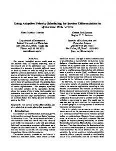
3.2 Structure of the fuzzy priority scheduler Based on the CAN mechanism, all the bits in the ID field are used to arbitrate the bus; that is, the message identifier is used as the secondary priority to compete the bus when two or more messages have the same priority level. In this case, priority inversion may result, which is key reason for QoS degradation of the network. Hence, the effects of the message identifier on the network performance should be considered. Other information about the broadcast characteristics of CAN play an important role, too. This information provides an estimation of the network status, for example, whether the network is idle, which node wins message arbitration, and which priority level the last transmitted message has. It makes it possible to set the priority of a message according to the network status, which hence forms a closed-loop feedback schedule. However, these two important factors are not considered in the existing dynamic schemes. In this paper, a new dynamic priority scheduling scheme based on fuzzy logic is constructed by using these factors. The structure of the fuzzy dynamic priority scheduler for node j is shown as Fig. 2. It has three inputs, LQS(j), Pri(i), and Id(j) and one output, Pri(j). LQS(j) reflects the laxity of different QoS requirements of a message. Id(j) is the message identifier. Pri(i) is the feedback input, which is the priority of a message from node i transmitted successfully last time. Pri(j) denotes the priority of a message for node j in the current contention determined by three pa-

Asian Journal of Control, Vol. 7, No. 4, December 2005

404

To enable faster execution of this fuzzy scheduler, the fuzzy inference mechanism based on Mamdani’s min implication and max-min composition, and the centroid of area method for defuzzification [19] are used. Therefore, the relationship between the output and inputs can be formulated similar to Eqs. (1) and (2). Priority is, thus, assigned nonlinearly.

Fig. 2. Structure of the fuzzy dynamic priority scheduler for node j.

rameters. It should be noted that, for node j, if the network is busy, the last recorded value of Pri(i) is used to encode its priority. On the other hand, if the network is idle, the historical value of Pri(i) is of no use any more and will be set to the lowest value possible.

3.3 Fuzzification, fuzzy inference and defuzzification Three verbal values are defined for each input/output. The verbal values for the linguistic variables Pri(i)/Pri( j), High, Medium, and Low, are defined in accordance with the CAN protocol. The trapezoidal membership functions are assigned to these verbal values, High, Medium, and Low, respectively, as shown in Fig. 3. The verbal values of Id( j) are Near, Medium, and Far. Two sigmoidal membership functions and one Π shape function are assigned to Near, Far, and Medium, respectively, as shown in Fig. 3. There are different QoS requirements for real-time and non-realtime messages; hence, different definitions for LQS( j) and the corresponding fuzzy scheduling rules should be specified separately, which will be discussed in the following two sections.

Fig. 3. Membership functions of Pri(i)/Pri(j) and Id(j).

Remark 2. Existing scheduling schemes [7-13] are openloop scheduling schemes. Because only the QoS requirements are considered in priority assignment, priority varies monotonically. In [14], the broadcast information was used as a control threshold; that is, a message with priority higher than this control threshold is allowed to solely compete for the network transmission. In this paper, broadcast information is used to set up a closed-loop scheduling scheme. Moreover, since fuzzy logic is used, priority can be assigned nonlinearly. The proposed scheme is feasible if the fuzzy chip is added to each CAN node. As for the CAN bus, the transmission time of the minimum CAN frame is 47 µs at a maximum speed of 1 Mbps. The inference speed of analog fuzzy chips is 1 or 2 Mega FLIPS (fuzzy logic inferences per second) [18], and that of digital fuzzy chips is 3.3 Mega FLIPS [19], so the processing overhead for fuzzy logic inferences is only 4.5 to 15 µs, which is much lower than the transmission time of the minimum CAN frame.

IV. FUZZY SCHEDULING FOR REAL-TIME MESSAGES In this section, the fuzzy input of LQS( j) is defined for a real-time message which reflects the transmission laxity. The performance and effectiveness of the proposed scheme were tested through simulation and are compared here with that of other dynamic priority scheduling schemes.

4.1 Fuzzy scheduling rules for real-time messages For real-time messages, LQS( j) is described as the current transmission laxity TL( j) of a message. TL( j) is defined as the difference between its relative deadline, rd( j), and its waiting time, tn(j) – tg( j), where tn( j) is the current instant and tg( j) is the generating instant of a message. To normalize TL( j), we introduce its bound, RTB (real time bound). That is, if the transmission laxity of a message exceeds this time horizon, its priority is set to the lowest level without using the fuzzy rules. Therefore, LQS( j) is defined as the ratio of TL( j) to RTB, as shown as Eq. (3). Three verbal values are defined for LQS( j): Urgent, Anticipant and Lax. The membership functions defined for Urgent and Lax are sigmoidal in form, and that for Medium is Π in shape, as shown as Fig. 4. The influence of RTB on the schedulable performance was tested through simulation:

T. Bai et al.: Flexible Fuzzy Priority Scheduling of the CAN Bus

Fig. 4. Membership functions of LQS(j) for real-time messages.

LQS ( j ) =

TL( j ) rd ( j ) − (tn ( j ) − t g ( j )) = . RTB RTB

(3)

Fuzzy scheduling rules for real-time messages are listed in Table 1. As Rule 1, LQS( j) in Eq. (3) is equal to Lax, which means that the QoS requirement of a message at node j is not critical now. The rule that Id(j) is Not Far means that the identifier of node j as the secondary priority is high, so it is more likely to win the competition. Therefore, no matter which priority level Pri(i) the last transmitted message had, setting a high priority Pri(j) for this message is not needed. However, if the priority Pri(i) is high, Pri( j) should be estimated based on the urgency of its message’s current LQS( j) and the value of its identifier Id( j), such as those of Rules 7, 8, 9, and 14. For example, with Pri(i) = Low, the priority for a message with Id(j) = Near will be set to a value in the set {4, 5, 6, 7} according to the urgency of its LQS(i), while the priority for a message with Id(j) = Far will be assigned a value in the set {2, 3, 4, 5}. Table 1. Fuzzy scheduling rules for real-time/non-real-time messages. Rule No. 1 2 3 4 5 6 7 8 9 10 11 12 13 14 15

LQS(j) Lax Lax Lax Anticipant Anticipant Anticipant Anticipant Anticipant Anticipant Urgent Urgent Urgent Urgent Urgent Urgent

Input Id(j) NotFar Far Far Near Medium Far Near Medium Far Near Medium Far Near Medium Far

Pri(i) − Low Not Low Not High Not High Not High High High High Low Not High Low Not Low High Not Low

Output Pri( j) Low Low Medium Low Medium Medium Medium Medium High Medium High High High High High

Weight 1 0.5 0.5 1 0.5 1 0.5 1 0.3 1 0.5 0.5 0.5 0.8 1

4.2 Simulation tests on real-time messages The network loads are listed in Table 2, where periods/minimum interarrival times (MIT) for periodic/aperiodic data and their corresponding deadlines are

405

given. The number of nodes in the tests is also given. The values marked with a ‘*’ are default values and were varied during the simulation. The length of each periodic message was 79 bits, which consisted of 32 bits of periodic data and 47 bits of frame overhead. The length of each aperiodic message, which was used to announce some event, was 47 bits with 0 bits of aperiodic data. In this study, bit-stuffing was not considered. Therefore, the transmission times for the above two kinds of messages were 79 µs and 47 µs, respectively, when the CAN bus with 1 Mbps was used. In the following simulation, RTB = 1500 µs was chosen for the fuzzy scheme. Table 2. Network load. Periodic Nodes No. of Period Deadline Nodes 4 1250 µs 500 µs 8* 1600 µs 700 µs* 2 2500 µs 1000 µs 2 5000 µs 2000 µs

Aperiodic Nodes No. of MIT Deadline Nodes 1s 2* 300* µs 50 ms 50 ms 1 200 ms 80 ms 1

In the following figures, EDF indicates the scheme with an infinite number of priority levels [20]. Fuzzy indicates the scheme proposed in this paper. LogEDF(k, q) is the practical EDF scheme in [10], where the maximum deadline is divided into k time sections logarithmically and each section is divided into q units of the same size, so there are (k × q) priority levels in total. LinearEDF(k) is the scheme used for high-speed messages in [7], where the deadlines are mapped into priorities using a linear scale with k priority levels. FTT-CAN is the scheme in [13], where the duration of an EC is set equal to the minimum deadline of the aperiodic messages. The length of the TM is

( ⎡⎢

N 8

)

⎤⎥ × 8 + 47 bits, where N is the number of periodic

nodes, 47 bits of the frame overhead, and ⎡⎢ z ⎥⎤ denotes that the elements of z are rounded off to the nearest integers greater than or equal to z. It is assumed that in each EC, only one aperiodic message is served. (1) Varying the number of periodic nodes The scheduling performance is shown as Fig. 5, where the number of periodic nodes with a period of 1600 s is varied; i.e., the network load changes from 34.89% to 104.02%. The difference in the scheduling performance between Fuzzy and EDF/LogEDF(16, 4) is only 0.01%, which is better than that of LogEDF(8, 8), while the performances of LogEDF(8, 1), LinearEDF(8) and LinearEDF(64) are worse. The performance of FTT-CAN is the worst, with the lowest percentages of schedulable messages. This is caused by the much higher overhead between 18.33% and 23.67%.

406

Asian Journal of Control, Vol. 7, No. 4, December 2005

(3) Varying the number of aperiodic nodes

Fig. 5. Performance comparison as the network load changes.

(2) Varying the deadlines of periodic nodes Figure 6 shows the scheduling performance when the deadlines of periodic messages with a period of 1600 µs are varied from 400 µs to 1600 µs. The scheduling perfor mance of Fuzzy and the LogEDF with 64 priority levels is very close to that of EDF. However, that of LogEDF(8, 1) and the LinearEDF with 8 or 64 priority levels is much worse; even though the deadlines reach 1600 µs, the system is still unchedulable. The difference between Fuzzy and EDF/LogEDF(16, 4) is only 0.04%, which is better than the LogEDF(8, 8) scheme. Similar to Fig. 5, the performance of FTT-CAN is the worst, with the lowest percentage of schedulable messages due to the higher overhead. As the above results show, though Fuzzy achieves scheduling performance close to that of EDF/LogEDF (16, 4), the number of unschedulable nodes with Fuzzy is greater than that with the other distributed schemes and smaller than that with FTT-CAN. That is, Fuzzy makes much more nodes get involved in the performance degradation of the network, which in some sense means that this scheme can serve the nodes more fairly.

The first row in Table 3 shows the network schedulability attained by varying the number of aperiodic nodes with an MIT of 1 s, when 3 periodic nodes with a period of 1600 µs and their deadlines 700 µs are chosen. When the number of aperiodic nodes is less than 4, the network is schedulable using EDF, LogEDF(16, 4) and Fuzzy with RTB equal to 1000/1500 µs. With Fuzzy with RTB equal to 2000 µs and LogEDF(8, 8), the network is schedulable only in the case with 2 aperiodic nodes. The choice of RTB for Fuzzy will affect the network performance. FTT-CAN1 is the scheme in which only one aperiodic message is served in each EC, while in FTT-CAN2, two aperiodic messages are served in each EC. This shows that for either of these FTT-CAN schemes, the scheduling performance with various numbers of aperiodic nodes is worse than the performance of other schemes. (4) Varying the deadlines of aperiodic nodes The second row in Table 3 shows the network schedulability when the deadlines of aperiodic nodes with an MIT of 1 s are varied, where 4 periodic nodes with a period of 1600 µs and deadlines of 700 µs are chosen. When the RTB for the Fuzzy scheme is chosen properly, the scheduling performance is similar to that of EDF/LogEDF(16, 4), which is better than that of LogEDF(8, 8). Note that by using the Fuzzy scheme with an RTB equal to 2000 µs and FTT-CAN1, the network is unschedulable, no matter how high the chosen deadlines. The minimum allowable deadlines for FTT-CAN2 are much higher than those for the other schemes. (5) Influence of RTB on the network performance The scheduling performance with different RTB values is shown in Fig. 7, when the deadlines of periodic messages with a period of 1600 µs vary from 400 µs to 1600 µs. If the chosen value of RTB is as small as 500 µs or larger than 3500 µs, the scheduling performance is much worse than that of EDF. The scheduling performance of the Fuzzy scheme with an RTB value between 1000 and 2000 µs is close to that of EDF; the difference is within 4%. Moreover, from Table 3, the network schedulability of the Fuzzy scheme with an RTB value between 1000 and 1500 µs is very close to that of EDF. Table 3. Schedulability test for varied parameters of aperiodic messages. Fuzzy Fuzzy (RTB = FTT LogEDF Log-EDF (RTB = 1000/ -CAN1 (8, 8) (16, 4) 2000 µs) 1500 µs) No. of Nodes 3 3 2 2 0 EDF/

Fig. 6. Performance comparison as deadlines change.

Deadline

730 µs

730 µs

−

890 µs

−

FTT -CAN2 − 950 µs

T. Bai et al.: Flexible Fuzzy Priority Scheduling of the CAN Bus

407

For non-real-time messages, three verbal values, Urgent, Anticipant, and Lax, are defined to represent LQS( j). The membership functions of Urgent and Lax are sigmoidal in form, and that of Anticipant is in the shape of a π curve, as shown as Fig. 8. Note that the membership value of 1 for Anticipant corresponds to the twice of the value of EAD. Fuzzy scheduling rules for non-real-time messages are equal to those for real-time messages, but their differences are the definition way of the linguistic variables of Urgent and Lax, shown as in Fig. 4 and Fig. 8.

5.2 Simulation tests on non-real-time messages Fig. 7. Performance comparison as RTB changes.

The results also show that the network has good performance if the RTB value is selected such that TL( j) takes 1.5 ~ 2 frame time units, and the corresponding grade of the membership function Urgent of LQS( j) is close to 1. From the above simulation tests, it can be seen that the proposed Fuzzy dynamic priority scheduling mechanism has network scheduling performance comparable with that of the EDF scheme with an infinite number of priority levels if the RTB value is properly chosen. The proposed Fuzzy scheme can use many fewer priority levels than the existing dynamic priority scheduling schemes and achieve better network schedulability.

The performance of non-real-time messages with this Fuzzy scheme was tested through simulation. It was assumed that there were 10 nodes in the network. Only non-real-time messages at each node needed to be served, and their traffic was assumed to follow a Poission distribution with an average arrival interval between 0.3 ms and 6 ms. The transmission time of a message was 79 µs when a maximum speed of 1 Mbps was used. Under different network load conditions, that is, light (36.62%), moderate (67.5%) and heavy (95.8%), the service fairness of nonreal-time messages with the Fuzzy control and round-robin scheduling schemes [5] was compared, and the results are shown in Fig. 9. Because the network bandwidth is allocated to each node evenly by the round-robin scheme, a node with a higher arrival rate may experience a longer

V. FUZZY SCHEDULING FOR NON-REAL-TIME MESSAGES One of the major aims of the proposed Fuzzy scheme is to guarantee fair service and the same QoS among nonreal-time messages and to balance the network load. Fig. 8. Membership functions of LQS(j) for non-real-time messages.

5.1 Fuzzy scheduling rules for non-real-time messages For non-real-time messages, LQS( j) is defined as the normalized delay of non-real-time messages; its current relative delay RD( j) is divided by the expected average transmission delay EAD of all messages as shown in Eq. (4). RD(j) is defined as the difference between its current waiting time, tn( j) – tg( j), and EAD, where tn( j) is the current instant and tg( j) is the generating instant of a message. If there are only non-real-time messages in the network and the traffic generated at each node exhibits a Poission distribution with an average arrival rate κi, the EAD can be calculated by Eq. (5), where C is the maximum message transmission time:

LQS ( j ) = EAD =

RD( j ) (tn ( j ) − t g ( j )) − EAD , = EAD EAD

2C − C 2 (∑ iN=1 κi ) 2(1 − C ∑

N i =1 κi )

.

(4) (5)

Fig. 9. QoS comparison of the Fuzzy control and round-robin schemes.

408

Asian Journal of Control, Vol. 7, No. 4, December 2005

network-induced delay. Therefore, the network load among different nodes is unbalanced. Compared with the roundrobin scheme, the proposed Fuzzy control scheme can guarantee a much better QoS. More bandwidth is allocated to a node with a higher arrival rate; hence, fair service and the same QoS for different nodes are obtained. Moreover, the network load is balanced.

VI. FLEXIBLE FUZZY SCHEDULING FOR NON-REAL-TIME MESSAGES In the above two sections, the QoS requirements of the nodes were assumed to be fixed, and the membership function of LQS( j) was defined with a fixed parameter of RTB or EAD. In fact, the nodes may have different QoS requirements that can change dynamically during run-time. It was also assumed in Section 4 that there were no real-time messages in the network and that the non-real-time traffic followed a Poisson distribution, whereas it is usual for realtime and non-real-time messages to coexist in a network, and the traffic may not really follow a Poisson distribution. It is hard to estimate the network loads and calculate the exact value of the fuzzy parameter, EAD, according to Eq. (5). Hence, in order to guarantee a flexible QoS requirement for each node and to make Fuzzy scheduling adaptable, it is necessary to develop an online updating algorithm for the fuzzy parameter. On the other hand, the game algorithm [15] has been used to optimize the network performance; for example, see [21] and the references therein. In the next part of this section, a non-cooperative fuzzy parameter control game (NFCG) is presented and proven to be stable and to converge at the Nash equilibrium [15]. Then, for non-real-time messages, an online updating algorithm for the fuzzy parameter, EAD, is proposed based on NFCG. Its effectiveness was tested through simulation, and the results are presented in the last subsection.

6.1 Existence and uniqueness of the nash equilibrium of NFCG In order to realize flexible network services, for each non-real-time node, the value of EAD must be set independently. Let xj > 0 be the selected value of EAD for node is the average transmission j. Its minimum bound x min j delay of node j without any other traffic in the network, and , is limited by the buffer capacthe maximum bound, x max j ity of node j. Simulation tests show that when the threshold xj increases, the average transmission delay of node j increases, while that of the other nodes i (≠ j) decreases. Because of the fuzzy control logic, the influence of xj on the average transmission delay of each node is complicated and hard to express formally. In order to prove the convergence and stability of the proposed updating algorithm, the virtual transmission delay of γj is defined as

γj =

g j xj

∑ ∀i ≠ j gi xi + σ j

,

(6)

where gi is the amplification of the threshold of xi and σj represents the influence of other factors on the transmission delay of node j. For node j, the utility function is defined as the difference between the basic utility of uˆ j and the cost of cj, i.e., u j = uˆ j − c j . The basic utility of uˆ j = log(a γ j + 1) , a ≥ 1 reflects its network QoS requirement, and as the virtual transmission delay increases, the network QoS requirement decreases; that is, the cost of running the network is reduced. The cost of cj = λj xj is the linear function of xj, which is the buffer overhead of node j. λj is its price factor; its different values reflect the different buffer costs of the nodes. Therefore, the updating scheme is a tradeoff between the cost of the network occupancy and the cost of the node buffer burden. The utility of node j is expressed as

u j = uˆ j − c j = log(a γ j + 1) − λ j x j ,

a ≥ 1.

(7)

As γj increases, the increase ratio of the utility of uj decreases, which complies with the rule of the decrease of the boundary utility. Definition 1. NFCG: NG = (Γ, {Xj}, {uj}) denotes the noncooperative fuzzy parameter control game (NFCG), where Γ = {1, 2, …, N} is the index set for the nodes in the CAN max ] ( x min > 0) is the strategy set and bus, X j = [ x min j , xj j

uj(⋅) is the utility function of node j. Each node selects its threshold level xj such that xj ∈ Xj. Let the threshold vector x = ( x1 , x2 , " , xN ) ∈ X denote the outcome of the game in terms of the selected threshold levels of all the nodes, where X is the set of all threshold vectors. The resulting utility level for node j is uj(x). An alternative notation, u j ( x j , x − j ) , is occasionally used, where x − j denotes the vector consisting of the elements of x other than the j th element. The latter notation emphasizes that the j th node only has control over its own threshold, xj. The strategy space of all the nodes, excluding the j th one, is denoted by X− j . In this non-cooperative game, each node maximizes its own utility in a distributed fashion. Formally, NFCG can be expressed as a constrained optimal problem:

max u j ( x j , x − j ),

x j ∈X j

∀j ∈ Γ ,

s.t . : x min ≤ x j ≤ x max . j j

(8)

The threshold that optimizes the individual utility depends on the thresholds of all the other nodes in the network. It is necessary to characterize a set of thresholds, where the nodes are satisfied with the utility they receive given the

T. Bai et al.: Flexible Fuzzy Priority Scheduling of the CAN Bus

threshold selections of other nodes. Such an operating point is called an equilibrium. Definition 2. Nash Equilibrium: A threshold vector of x = (x1, x2, …, xN) is the Nash equilibrium of NFCG NG = (Γ, {Xj}, {uj(⋅)}), if for every j ∈ Γ, u j ( x j , x− j ) ≥ u j ( x′j , x− j ) for all x′j ∈ Xj. At a Nash equilibrium, after the threshold levels of the other players are given, no user can improve its utility level by making individual changes in its threshold. The threshold level chosen by a rational self-optimizing user constitutes the best response to the thresholds that have been actually chosen by other players. The Nash equilibrium concept offers a predictable, stable outcome of a game where multiple agents with conflicting interests compete through self-optimization and reach a point where no player wishes to deviate. However, such a point does not necessarily exist and is not unique at all times. In the following, we will investigate the existence and uniqueness of the Nash equilibrium in NFCG. Theorem 1. A Nash equilibrium exists in the NFCG, NG = Γ, {Xj}, {uj(⋅)}. The proof of the above theorem can be found in Appendix A. The set of maximizers of the continuous function u j ( x j , x − j ) on the compact set Xj in NFCG is called the best-response correspondence and is denoted by rj (x − j ) . It is the mapping rj : X − j → X j and is defined as [16]

rj (x − j ) = {x j ∈ X j : u j ( x j , x − j ) ≥ u j ( x′j , x − j ), ∀x j ∈ X j } . (9) An alternative definition for the Nash equilibrium can be stated using the set of best responses. A threshold vector x is a Nash equilibrium of NFCG if and only if x j ∈ rj (x − j ) for all j ∈ Γ. When the conditions in Theorem 11 [21] are satisfied, the correspondence rj (x − j ) is nonempty, convex-valued and upper semi-continuous for all j. Thus, there exists a fixed point x such that x j ∈ rj (x − j ) for all j ∈ Γ. This fixed point is, by definition, a Nash equilibrium. The above theorem expresses the existence of a Nash equilibrium in NFCG, where the utility function is quasiconcave in the threshold. At this point, it is important to make a statement of equilibrium existence in general. An equilibrium existence proof states that under certain conditions, an equilibrium is guaranteed to exist. Such a statement does not imply, however, that if the same conditions are not met, no equilibrium exists. The properties of the equilibrium itself will be discussed below. First, the best-response correspondence of a node in NFCG will be derived.

409

Proposition 2. In NFCG, node j′s best response to a given vector x − j is given as max rj (x) = min(max( x min ˆ j ), x j ) , j , x

where

xˆ j = arg max x j ∈R+ (u j ( x j , x − j ))

represents the

unconstrained maximizers of the utility in Eq. (7). Furthermore, xˆ j =

1 λj

−

∑ ∀i ≠ j gi xi +σ j ag j

, (λ j ≠ 0) is unique.

The proof of the above theorem can be found in Appendix B. Note that at any equilibrium of the NFCG game, a node either attains the maximal utility, or it fails to do so and transmits the data at its maximum or minimum threshold. Theorem 3. NFCG has a unique equilibrium. The proof of the above theorem can be found in Appendix C. The existence and uniqueness of the Nash equilibrium in NFCG ensure that the updating algorithm based on NFCG is stable and convergent.

6.2 Fuzzy parameter updating algorithm The online updating algorithm for the fuzzy parameter based on NFCG is realized by calculating the fixed point equation x(t) = r((x)(t − 1)). The virtual average transmission delay of node j is replaced with its real average transmission delay, which can be measured by itself. Between two updating instants, the threshold of xj is constant; thus the fixed point equation can be expressed as

⎛ ⎛ xj 1 rj (x) = min ⎜ max ⎜ x min − j , ⎜ ⎜ λ j aθ j ⎝ ⎝

⎞ max ⎞ ⎟⎟ , x j ⎟ , ⎟ ⎠ ⎠

(10)

where θj is the real average transmission delay of node j. It should be noted that the fixed point Eq. (10) is no longer related to the parameters of gj, gi (i ≠ j) and σj. Therefore, though the expression of γj is based on observation and only reflects the coarse relationships between the thresholds and the node’s transmission delay, it causes no problems for accurate expression of the fixed point equation because of the complete substitution with its real average transmission delay. The cost factor of λj can be fixed or changed, depending on the desired buffer cost of the node. When all nodes wish to get network fairness even though the network loads are fluctuating, the cost factor of λj is determined as follows:

λj =

a a θˆ j + 1

,

(11)

where θˆ j is the total average transmission delay. Based on the above analysis, the online updating algorithm for the fuzzy parameter is listed as follows:

410

Asian Journal of Control, Vol. 7, No. 4, December 2005

1. Initialize the threshold vector x(t) and the precision of ε > 0 with the initial instant t = 0; 2. let t = t + 1; calculate x = r(x(t − 1)) with the fixed point Eq. (10); 3. for all j, if | xj(t) − xj(t − 1) | > ε; then, return to step 2, else x(t) is optimal value. This algorithm is feasible while not much computation load is imposed on the node.

6.3 Simulation tests on the updating algorithm It was assumed that there were 10 nodes in the network and that the network load varied. The transmission time of a message was 79 µs with a maximum network speed of 1 Mbps. Only non-real-time messages at each node needed to be served, and their corresponding traffic was assumed to follow a Poission distribution with an average arrival interval between 0.25 ms and 3 ms. The parameter a in the fixed point Eq. (10) was equal to 1. The initial thresholds were between 100 µs and 600 µs. It was assumed that the transmission delay of the data from other nodes was determined using the time stamping method. Hence, the cost factor of λj could be calculated online using Eq. (11). At a simulation time of 2 s, the network load changed from 67.5% to 83.56%. It is shown in Fig. 10 that no matter how the network load changed, the threshold and the utility of each node could be kept at a steady value. Although the network load is hard to estimate, the Fuzzy control scheme with the online updating algorithm can still ensure fairness and the same QoS for non-real-time messages, because all non-real-time messages have the close utility values.

tributed real-time control systems. However, the bus arbitration mechanism must be used properly, with careful design of the message ID; otherwise, CAN will result in low utilization. In this paper, a new closed-loop scheme based on fuzzy dynamic priority scheduling has been proposed. It uses the broadcast nature of the CAN bus. Besides the QoS requirements of a message, the message identifier and the feedback information about the network status are utilized in the Fuzzy priority scheme to provide a nonlinear priority encoding method. Simulation results show that the proposed Fuzzy scheduling scheme uses fewer bits to encode fewer priority levels, which makes the service range of the network wide without increasing the overhead, compared with the dynamic priority schemes. Moreover, the game algorithm is used to adjust the fuzzy parameter, which makes the algorithm flexible and guarantees the QoS of the network, even with fluctuating traffic. Simulation results have well demonstrated the ability of the Fuzzy scheme to guarantee high schedulability for real-time messages, as well as fairness and the same QoS for non-realtime messages in networks.

APPENDIX A.1 Proof of Theorem 1 Proof. The following result is obtained from [21]. Theorem 11. [21] A Nash equilibrium exists in a game NG = (Γ, Xj, uj(⋅)), j ∈ Γ if for all j ∈ Γ, 1. Xj is a nonempty, convex and compact subset of some Euclidean space RN; 2. u(x) is continuous in x and quasi-concave in xj. The proof of the theorem is completed by showing that the conditions given above are met in NFCG. Each node has a max ] ( x min > 0) , and all the threshstrategy space [ x min j , xj j

old values are in it. It is also assumed that the maximum threshold is larger than or equal to the minimum threshold; thus, the first condition is satisfied. It remains to show that the utility function uj(x) is quasi-concave in xj for all j ∈ Γ in NFCG. Firstly, the quasi-concavity is defined. Definition 3. The function u j : X j → R+1 defined on the convex set Xj is quasi-concave in xj if and only if

u j = (βx j + (1 −β) x′j , x− j ) ≥ min(u j ( x j , x − j ), u j ( x′j , x − j )) for xj, xj ∈ Xj, β ∈ [0, 1].

The first partial derivative of uj(⋅) with respect to xj is Fig. 10. Performance of updating algorithm with variable workloads.

VII. CONCLUSION AND FUTURE WORK Because of the attractive features of CAN, such as short worst-case bus access latency and its priority-based bus access mechanism, the CAN bus is widely used in dis-

∂u j ( x j , x − j ) ∂x j

=

ag j ag j x j + ∑ ∀i ≠ j gi xi + σ j

−λj .

(12)

The second partial derivative of uj(⋅) with respect to xj is

∂u 2j ( x j , x − j ) ∂x 2j

=−

(ag j ) 2 (ag j x j + ∑ ∀i ≠ j gi xi + σ j ) 2

< 0. (13)

T. Bai et al.: Flexible Fuzzy Priority Scheduling of the CAN Bus

By Eq. (13), the utility function uj(⋅) is concave in xj. Because the concave function is also quasi-concave, the utility function uj(⋅) is quasi-concave in xj, too. Hence, the second condition is satisfied. This completes the proof of the theorem.

Proof. Given the thresholds of the other nodes, the optimal threshold or the equilibrium of node j is obtained by solving the constrained optimal problem described by Eq. (8). Its associated Lagrangian is given by

L j = u j ( x j , x − j ) − µ1 ( x min − x j ) − µ 2 ( x j − x max ) , (14) j j where µ1 and µ2 are the Lagrange multipliers. xj* is, thus, an equilibrium point if and only if it satisfies the Kuhn-Tucker conditions, that is,

ag j + (∑ ∀i ≠ j gi xi + σ j ) − λ j + µ1∗ − µ∗2

µ1∗ ( x min j

−

x∗j )

=0,

=0,

µ∗2 ( x∗j − x max ) =0, j µ1∗ , µ∗2 ≥ 0 .

(15)

Case 1: when µ1∗ ≠ 0, µ∗2 ≠ 0 , there is not solution. Case 2: when

µ∗2 = ∂u j (⋅) ∂x j

µ1∗ = 0, µ∗2 ≠ 0 , then ag j ag j x max + ( ∑ ∀i ≠ j gi xi +σ j ) j

function uj(⋅) is strictly concave from Eq. (13), xˆ j is

Proof. By Theorem 1, we know that there exists an equilibrium in NFCG. Let x denote the Nash equilibrium in NFCG. By definition, the Nash equilibrium has to satisfy x = r(x), where r(x) = (r1(x), r2(x), …, rN(x)). Note that rj(x) and rj (x − j ) are equivalent. The key point of the uniqueness proof is that the best-response correspondence r(x) is a standard function [22]. A function is said to be standard if it satisfies the following properties. 1. Positivity: r(x) > 0. 2. Monotonicity: If x ≥ x′, then r(x) ≥ r(x′) or r(x) ≤ r(x′). 3. Scalability: For all α > 1, αr(x) > r(αx). It is assumed that the system is feasible; that is, each node can obtain the determinate utility by setting some threshold to control the transmission of its data. Hence, r(x) satisfies the positivity condition. To prove that r(x) achieves monotonicity and scalability, those for the boundary points are proven firstly. If

rj (x) = x max or rj (x) = x min , then rj(x) = rj(x′) when x ≥ j j requirement.

Because

is monotonic decreasing because of the con∂u j ( ⋅) |x j = xˆ j = ∂x j

0,

> 0 for x min ≤ x j ≤ x max , that is, µ∗2 > 0 , j j

µ1∗ =

µ1∗ ≠ 0, µ∗2 = 0 , then ag j ag j x min j + ( ∑ ∀i ≠ j gi xi +σ j )

Similarly, ∂u j ( ⋅) ∂x j

if

guaranteed. Now, we will discuss the monotonicity and scalability for the case of rj (x) = xˆ j . For x ≥ x′,

rj x − rj x′ =

with

∂u j (⋅) | = ∂x j x j = xˆ j

=

is the K-T point. then x∗j = x min j 1 λj

−

∑ ∀i ≠ j gi xi +σ j ag j

,

(λ j ≠ 0) is the K-T point. Therefore, the best response of node j is calculated as

⎞ ⎟⎟ ⎠

∑ ∀i ≠ j gi ( xi′ − xi )

0 ,

< 0 for x min ≤ x j ≤ x max , that is, µ1∗ > 0 , j j

Case 4: when µ1∗ = 0, µ∗2 = 0 , x∗j = xˆ j =

1 ∑ ∀i ≠ j gi xi + σ j − λj ag j

⎛ 1 ∑ ∀i ≠ j gi xi′ + σ j −⎜ − ⎜λj ag j ⎝

x∗j = x min , and j

+λj .

min xˆ j ≤ x j

αrj (x) = αx max > x max = r j (αx ) j j

or αrj (x) = αx min > x min = rj (αx) , the scalability is also j j

−λj .

is the K-T point. then x∗j = x max j Case 3: when

■

unique. This completes the proof of the proposition.

x′; that is, the boundary point satisfies the monotonicity

x∗j = x max , and j

with cavity of uj(⋅). If xˆ j ≥ x max j ∂u j ( ⋅) ∂x j

max rj (x) = min(max( x min ˆ j ), x j ) . Because the utility j , x

A.3 Proof of Theorem 3

A.2 Proof of Proposition 2

ag j x∗j

411

ag j

≤0,

(16)

so r(x) is monotonic. Because the system is feasible, uj = log(aγj + 1) − λj xj > 0; then,

⎛ ⎞ ag j x j λ j x j < log ⎜ + 1⎟ < ⎜ ∑ ∀i ≠ j gi xi + σ j ⎟ ⎝ ⎠

ag j x j

∑ ∀i ≠ j gi xi + σ j

,

Asian Journal of Control, Vol. 7, No. 4, December 2005

412

1 > λj

∑ ∀i ≠ j gi xi + σ j ag j

>

σj ag j

.

(17)

9. Livani, M.A., J. Kaiser, and W.J. Jia, “Scheduling Hard and Soft Real-Time Communication in a Controller Area Network,” Contr. Eng. Pract., Vol. 7, pp. 1515-1523 (1999).

Hence,

α r j ( x ) − r j (α x ) =

α α(∑ ∀i ≠ j gi xi + σ j ) − λj ag j ⎛ 1 ∑ ∀i ≠ j gi (αxi ) + σ j −⎜ − ⎜λj ag j ⎝

10. Natale, M.D., “Scheduling the CAN Bus with Earliest Deadline Techniques,” Proc. Real-Time Syst. Symp., pp. 259-268 (2000).

⎞ ⎟⎟ ⎠

⎛ 1 σj ⎞ = (α − 1) ⎜ − ⎜ λ j ag j ⎟⎟ ⎝ ⎠ >0,

on Computer Science, Vol. 1985, Languages, Compliers and Tools for Embedded Systems, in ACM SIGPLAN Workshop LCTES’2000, pp. 1-18 (2001).

(18)

so r(x) is scalable. In conclusion, r(x) is a standard function, and the fixed point x = r(x) is unique. Therefore, the Nash equilibrium of NFCG is unique.

REFERENCES 1. Altman, E., T. Basar, and R. Srikant, “Nash Equilibria for Combined Flow Control and Routing in Networks: Asymptotic Behavior for a Large Number of Users,” IEEE Trans. Automat. Contr., Vol. 47, No. 6, pp. 917930 (2002). 2. Altman, E., “Nash Equilibria in Load Balancing in Distributed Computer Systems,” Int. Game Theory Rev., Vol. 4, No. 2, pp. 1-10 (2002). 3. Road Vehicles ⎯ Interchange of Digital Information ⎯ Controller Area Network (CAN) for High-Speed Communication, International Standards Organisation (ISO), ISO Standard-11898 (1993). 4. Farsi, M., K. Ratcliff, and M. Barbosa, “An Overview of Controller Area Network,” Comput. Contr. Eng. J., Vol. 10, No. 3, pp. 113-120 (1999). 5. Hansson, H.A., T. Nolte, C. Norstrom, and S. Punnekkat, “Integrating Reliability and Timing Analysis of CAN-Based Systems,” IEEE Trans. Ind. Electron., Vol. 49, No. 6, pp. 1240-1250 (2002). 6. Torngren, M., “A Perspective to the Design of Distributed Real-Time Control Applications Based on CAN,” http://www.damek.kth.se, Oct. 6 (2003). 7. Zuberi, K.M. and K.G. Shin, “Design and Implementation of Efficient Message Scheduling for Controller Area Network,” IEEE Trans. Comput., Vol. 49, No. 2, pp. 182-188 (2000). 8. Bello, L.L. and O. Mirabella, “Randomization-Based Approaches for Dynamic Priority Scheduling of Aperiodic Messages on a CAN Network,” Lecture Notes

11. Nolte, T., M. Sjodin, and H. Hansson, “Server-Based Scheduling of the CAN Bus,” Proc. 9th IEEE Int. Conf. Emerging Technol. Fact. Autom. (ETFA03), Calouste Gulbenkian Foundation, Vol. 1, Lisbon, Portugal, pp. 169-176 (2003). 12. Nolte, T., M. Sjodin, and H. Hansson, “Hierarchical Scheduling of CAN Using Server-Based Techniques,” Proc. 3rd Int. Workshop Real-Time Networks (RTN’04) & 16th Euromicro Int. Conf. Real-Time Syst. (ECRTS 2004), Catania, Italy (2004). 13. Pedreiras, P. and L. Almeida, “EDF Message Scheduling on Controller Area Network,” Comput. Contr. Eng. J., Vol. 13, No. 4, pp. 163-170 (2002). 14. Cena, G. and A. Valenzano, “Achieving Round-Robin Access in Controller Area Networks,” IEEE Trans. Ind. Electron., Vol. 9, No. 6, pp. 1202-1213 (2002). 15. Zhang, W.Y., Game Theory & Information: Economics, Chapter 1, San Lian Bookstore Press & Shanghai People’s Press, Shanghai, China (1996). 16. Stobart, R., “Tutorial on Fuzzy Control,” IEE Colloquium on Two Decades of Fuzzy Control ⎯ Part 1, Vol. 1, pp. 1-6 (1993). 17. Wang, L.X., A Course in Fuzzy Systems and Control, in Chinese, Tsinghua University Press, Beijing (2003). 18. Snchez-Solano, S., A. Barriga, C.J. Jimnez, and J.L. Huertas, “Design and Application of Digital Fuzzy Controllers,” Proc. 6th IEEE Int. Conf. Fuzzy Syst., Vol. 2, Barcelona, pp. 869-874 (1997). 19. Hung, D.L, “Dedicated Digital Fuzzy Hardware,” IEEE Micro, Vol. 15, No. 4, pp. 31-39 (1995). 20. Georges, L., P. Muhlethaler, and N. Rivierre, “A Few Results on Non-Preemptive Real Time Scheduling,” http://www.inria.fr/rrrt/rr-3926.html (2000). 21. Saraydar, C.U., N.B. Mandayam, and D.J. Goodman, “Efficient Power Control via Pricing in Wireless Data Networks,” IEEE Trans. Commun., Vol. 50, No. 2, pp. 291-303 (2002). 22. Yates, R.D., “A Frame for Uplink Power Control in Cellular Radio Systems,” IEEE J. Sel. Area Comm., Vol. 13, No. 7, pp. 1341-1347 (1995).

T. Bai et al.: Flexible Fuzzy Priority Scheduling of the CAN Bus

Tao Bai received her M.S. degree in 2001 in industry automation. She was with the Department of Automation, Tai Yuan Heavy Machinery Institute, China. Now she is with the Department of Automation, Shanghai Jiao Tong University, as a Ph.D. candidate. Her research interests include industrial networked system modeling, control and optimization.

Li-sheng Hu received his Ph.D. degree in the field of industrial automation from Zhejiang University, Hangzhou, China, in 1998. He is now a professor in the Department of Automation, Shanghai Jiao Tong University. His research interests are in the area of robust model prediction control, process monitoring, control performance limitation, and sampled-data control.

Zhiming Wu received his B.S. degree in electric engineering from Shanghai Jiao Tong University, China, in 1959. He is now a professor in the Department of Automation, Shanghai Jiao Tong University. His research interests include hybrid dynamic systems, distributed realtime embedded systems and information integration.

413

Genke Yang received his Ph.D. degree in system engineering from Xi An Jiao Tong University, China, in 1998. He is now a professor in the Department of Automation, Shanghai Jiao Tong University. His research interests include complex system control and optimization, and manufacturing system scheduling and management.