flow and turbulence in sharp open-channel bends

FLOW AND TURBULENCE IN SHARP OPEN-CHANNEL BENDS

THÈSE NO 2545 (2002) PRÉSENTÉE À LA FACULTÉ ENAC SECTION DE GÉNIE CIVIL

ÉCOLE POLYTECHNIQUE FÉDÉRALE DE LAUSANNE POUR L'OBTENTION DU GRADE DE DOCTEUR ÈS SCIENCES

PAR

Koen BLANCKAERT Burgerlijk Bouwkundig Ingenieur, Universiteit Gent, Belgique DEA de mécanique, Université C. Bernard, Lyon I, France et de nationalité belge

acceptée sur proposition du jury: Prof. W.-H. Graf, directeur de thèse Prof. H.-J. De Vriend, rapporteur Prof. W.-H Hager, rapporteur Prof. P.-A. Monkewitz, rapporteur Prof. A. Schleiss, rapporteur Prof. Y. Zech, rapporteur

Lausanne, EPFL 2003

“ Wer dies Wasser und seine Geheimnisse verstünde, so schien ihm, der würde auch viel anderes verstehen, viele Geheimnisse, alle Geheimnisse.” From Siddharta by Hermann Hesse

Aan mijn ouders, Aan Beril

Acknowledgements Towards the end of this PhD, I can look back on a period rich of experiences and satisfaction. Though writing a PhD is by definition an individual work, contributions by a lot of people are essential for its success. My most respectful thanks are due to my supervisor, Prof. W.H. Graf, for having given me the opportunity to work in Lausanne. I especially want to acknowledge him for his confidence, the academic liberty he gave me, and for having introduced me in academia. I am grateful to Prof. A.J. Odgaard (Iowa University, USA) for his decisive contributions in defining the subject and objectives of this PhD. I had the chance to work with a brilliant man as Prof. H.J. de Vriend (Techn. Univ. Delft, The Netherlands), who – although not officially - is the co-supervisor of this PhD. His contributions were of fundamental importance for this dissertation. He co-authored papers III.2,3,4 and improved papers II.1 and III.1. My appreciation and thanks simply cannot be put into words. The experimental part of this PhD relies on a high-tech instrument, the Acoustic Doppler Velocity Profiler, developed in our laboratory under the supervision of Dr. U. Lemmin. I am indebted to him for having given me the opportunity to use this instrument and for having accepted to co-author paper I.1. Thanks are due to R. Fontanellaz for his invaluable advice in conceiving and constructing the experimental infrastructure and to C. Perrinjacquet for keeping the computer resources operational. Numerical simulations have been carried out in collaboration with Prof. S.S.Y. Wang and Prof. Y. Jia (Mississippi Univ, USA) that resulted in the joint paper IV.2. I am grateful to them for this fruitful collaboration. I acknowledge Prof. I. Nezu (Kyoto Univ., Japan) and Dr. R. Booij (Techn. Univ. Delft, The Netherlands) for their willingness to review and improve parts of this dissertation. I was honored by the acceptance of Prof. A. Schleiss (EPFL), Prof. P.A. Monkewitz (EPFL), Prof. W.H. Hager (ETH Zürich), Prof. Y. Zech (Univ. Louvain, Belgium) and Prof. H.J. de Vriend (Techn. Univ. Delft, The Netherlands) to serve on the doctoral committee. My gratitude is due to the Swiss National Science Foundation for having funded this research during the period May 1998-January 2002. Acknowledgements are also due to Dr. M. Altinakar, who is presently acting director of our laboratory, for his continuing support. Furthermore, I thank my colleagues P. Aviolat, M. Cellino, I. Fer, Y. Guan, D. Hurther, I. Istiarto, R. Jiang, A. Kurniawan, B. Özen, Z. Qu, I. Schoppe, W. Shen, L. Umlauf and B. Yulistiyanto for creating a fruitful working environment, as well as my friends for making life in Lausanne enjoyable. Finally, my most heartfelt thanks go to my parents and my girlfriend Beril. I will never forget their faithful travels to Lausanne, their unconditional support and their love.

VERSION ABRÉGÉE

i

Summary The sustainable development of rivers requires a knowledge on the three-dimensional mean flow field and the turbulence in complex morphologies. In a future, the computational capacity will be sufficient to simulate numerically the fine details of the flow. Our physical knowledge, however, is at present insufficient: the overwhelming majority of experimental research concerns straight-uniform flow and even complex numerical models are based on straight-uniform-flow knowledge. A sound understanding of the relevant physical processes will always be essential in complicated problems such as the river management, which concern a variety of different fields, and this irrespective of the available computational capacity. This PhD investigates, mainly experimentally, the mean-flow field and the turbulence in open-channel bends; this situation is considered as a generic case for complex highly three-dimensional flow. The experimental investigation is rendered feasible by the availability of a powerful Acoustic Doppler Velocity Profiler (ADVP), developed in our laboratory. The principal objectives of this PhD are: - To provide a high-quality data base on three-dimensional open-channel flow, including all three mean velocity components and all six Reynolds stresses on a fine grid. - To document interesting features of the flow field and the turbulence, such as the multi-cellular pattern of secondary circulation, the curvature influence on the turbulence, etc. - To gain insight in the relevant physical mechanisms and processes underlying these features. - To apply the acquired knowledge in an engineering sense, mainly by evaluating, improving and developing numerical simulation techniques. First, a limited series of experiments was conducted in a small laboratory flume, with the aim of testing the feasibility of the project. Subsequently, extended series of experiments have been designed in a large and optimized laboratory flume. The small-flume experiments yielded results beyond all expectations and form the core of this dissertation. The large-flume experiment are intended to confirm those results and to investigate newly emerged questions. Only few large-flume results are included in this dissertation; more large-flume results will be reported in literature in the future.

The structure of this dissertation follows the above-mentioned objectives. In PART I “Instrumentation and experimental set-up”, the experimental set-up, the ADVP and the measuring strategy are presented. Furthermore, a method is proposed to improve acoustic turbulence measurements.

ii

PART II “Experimental observations” provides high-quality data on the mean flow and the turbulence and documents the most interesting features: (i)

The downstream velocity increases in outward direction and its vertical profiles are flatter (increased/decreased velocities in the lower/upper part of the flow depth) than in straight flow.

(ii)

A relatively small and weak outer-bank cell of secondary circulation exists besides the classical center-region cell (helical motion).

(iii) The turbulence activity is reduced in the outer half of the cross-section in the investigated bend, as compared to a straight-uniform flow. (iv) Linear models that are commonly used to account for the effect of the secondary circulation in depth-integrated flow models are inaccurate for moderately to strongly curved flows.

PART III “Fundamental research” investigates the physical mechanisms and processes underlying these observations, mainly by making term-by-term evaluations of the relevant flow equations (momentum, vorticity, turbulent kinetic energy) and by considering the instantaneous flow behavior. The distribution of the downstream velocity is dominated by both cells of secondary circulation, whereby the outer-bank cell has a protective effect on the stability of the outer bank by keeping the core of maximum velocity at distance. The center-region cell is mainly generated by the vertical gradient of the centrifugal force, (∂/∂z)(vs2/R): the non-uniform outward centrifugal force and the nearly-uniform inward pressure gradient, due to the super-elevation of the water surface, are on the average in equilibrium; their local non-equilibrium, however, gives rise to the centerregion cell. There exists a strong negative feedback between the vertical profile of the downstream velocity, vs, and the center-region cell: the center-region cell flattens the vsprofiles, which on its turn leads to a reduction of (∂ / ∂ z)(vs2/R) and a weakening of the center-region cell. Linear models that are commonly used to account for the effect of the secondary circulation in depth-integrated flow models perform poorly because they neglect this feedback. Similar outer-bank cells exist in straight turbulent flow as well as in curved laminar flow. In straight turbulent flow, they are induced by the anisotropy of turbulence whereas they come into existence in curved laminar flow when the curvature exceeds a critical value: the vs-profiles flatten to such an extent that the gradient of the centrifugal force changes sign near the water surface, (∂/∂z)(vs2/R) 10 Hz. Correspondingly, the cumulative spectrum has an “S” shape for f < 10 Hz and only starts to deviate slightly for f > 10 Hz. Fig. 8a, and especially Fig. 8b, show that a considerable improvement is obtained by estimating the turbulent normal stress v x′2 from the redundant velocity information as ′2 . Although the estimate v˜x′ 1v˜x′ 2 v˜x′ 1v˜x′ 2 instead of from only one velocity information as v˜x1 should theoretically be free of parasitical noise, Figs. 8a and b indicate a remaining noise contribution in the high frequency range. However, this noise level is about one order of ′2 . As a result, the useful frequency magnitude smaller than the original noise level of v˜x1 range where noise contributions are small has been extended by about an order of magnitude by applying the noise correction method. In the example given in Figs. 8a,b, a parasitical noise contribution remains for f > 10 Hz. This limiting frequency depends on the SNR and thus on the acoustic scattering level of the fluid. This will be further discussed below. The above results indicate that by simply optimizing the ADV configuration with four receivers, the parasitical noise on turbulence measurements can largely be eliminated. Obviously, the turbulence characteristics can be obtained in any other reference system by applying a coordinate transformation.

I.26 3.3.2

Discussion of results

In the following, we will focus on two important points that are rarely discussed in the literature: (i) What measuring frequency should be chosen in ADV turbulence measurements ? As mentioned before, the measuring frequency of the ADVP is given by prf/NPP. Here, the measurements will by treated with NPP=16, yielding a measuring frequency of 62.5 Hz. The cospectra and the cumulative cospectra of the three almost noise free turbulent ′ v˜y2 ′ and v˜z1′ v˜z2′ are given in Figs. 9a,b. The ′ v˜x2 ′ , v˜y1 normal stresses, estimated as v˜x1 cospectrum of v˜z1′ v˜z2′ clearly shows a zone with a –5/3-slope and does not contain any parasitical noise tail. Its slope even gets steeper in the high frequency range. The ′ v˜x2 ′ corresponding cumulative cospectrum has a typical “S” shape. The cospectra of v˜x1 ′ v˜y2 ′ also show a zone with a –5/3 slope but they contain a remaining high and v˜y1 frequency noise tail for f > 10 Hz. This noise tail is clearly discernible in the cumulative cospectra, that have the typical shape for f < 10 Hz, but start to deviate for f > 10 Hz. The reason that the vertical turbulent normal stress v˜z1′ v˜z2′ has better noise characteristics ′ v˜y2 ′ is purely geometrical. The horizontal velocity ′ v˜x2 ′ and v˜y1 than the horizontal ones v˜x1 components are calculated from the difference between measured Doppler frequencies, whereas the vertical ones are obtained from their sum (cf. Fig. 4), which is less sensitive to error propagation. 2.5

-2

10 -3 10 -1

2

2 3

2 *

0

Sx1, x2 u∗2

2

Sy1, y 2 u∗2

3

Sz1, z2 u∗2 10 0

b

1

slight noisecontribution 1.45 estimation of noise-free profile based on highfrequency tail of 3

10 1

10 2

0.82 0.71 0.55

2 3

0.5

f [Hz]

0 10 -1

2.40 2.25

1

1.5

ij

1

v˜x′ 1v˜x′ 2 u∗2 v˜y′ 1v˜y′ 2 u∗2 v˜z′1v˜z′2 u∗2

0

10 -1

10

-5/3

f

10

2 3

∫ S (f´ )df´ u

2 Sij u* [Hz-1 ]

10 1

1

10 0

f [Hz]

10 1

f N = 31 25

1

[ /]

a

f N = 31 25

10 2

10 2

Fig. 9: Normalized power cospectra (a) and cumulative power cospectra (b) of v˜x′ 1v˜x′ 2 , ′ v˜y2 ′ and v˜z1′ v˜z2′ v˜y1 With a measuring frequency of 62.5 Hz, v x′2 and v y′2 are clearly overestimated. Fig. 9b further indicates that increasing the measuring frequency would result in an important deterioration of the estimates, since the parasitical noise tail tends to “explode”. Taking too low a measuring frequency instead can result in considerable underestimates, since most of the energy is contained in the inertial subrange . For example, when estimating ′2 , the low noise range is limited to f < 1 Hz the longitudinal turbulent normal stress as v˜x1 (Fig. 8), which would lead to an underestimate of about 35% (cf. Fig. 9b). Figs. 9 a,b

I.27 demonstrate that good estimates are obtained by choosing the “cut-off” measuring frequency in the flat part of the cumulative (co)spectrum before the noise tail becomes important. For the considered example, good estimates are obtained with a measuring frequency of 31.25 Hz (NPP=32, corresponding to a Nyquist frequency of 15.6 Hz). Obviously, the choice of the optimal measuring frequency is case- and instrumentdependent and is based on the knowledge of the noise levels. If the SNR level is too low, ′2 , and the flat part in the cumulative spectrum is not reached as is the case in Fig. 8b for v˜x1 accurate estimates of the turbulent normal stresses are not possible. The next section presents and illustrates a technique to increase the SNR.

(ii) What is the influence of a relatively low measuring frequency on the turbulence results ? Obviously, the accuracy of ADV turbulence measurements depends on: - The characteristic lengthscales of the flow, - The acoustic scattering level of the fluid, - The measuring frequency - The characteristics of the ADV The effect of most of these aspects can only be roughly estimated. In the above example, good turbulence results are obtained with a measuring frequency of 31.25 Hz in a flow with a relatively high acoustic scattering level. The accuracy estimates indicated in Fig. 9b correspond to the accuracy estimate of O(10%) given by Hurther and Lemmin (2001). Typically, the measuring frequency with ADV instruments is O(20 Hz), and the corresponding Nyquist frequency (maximum frequency for which the power spectral density can be estimated) is O(10 Hz). Taylor has defined a microscale of turbulence as λ = 15 ν v x′2 ε with ε the dissipation rate, which is a characteristic scale for the small turbulent eddies that dissipate energy. Using Taylor’s frozen turbulence hypothesis, Eq. 16, the corresponding frequencies can be estimated as f λ = (v x 2 π ) λ . In the spectral space, these small eddies are found at the high frequency end of the –5/3-slope region. As mentioned above, this inertial subrange is followed by a viscous range where the slope is steeper than –5/3 due to dissipation. Nezu and Nakagawa (1993) propose different methods to experimentally estimate λ , all of which resulted in fλ=O(10 Hz) for the investigated flow. This complies with Fig. 9a, where the slope of the spectrum at fN=31.25 Hz is already steeper than –5/3. The presented ADVP measurements thus cover the entire inertial subrange and even the beginning of the viscous range. In general, the extent of the inertial subrange in the frequency domain depends on the specific flow conditions, and especially on the Reynolds number of the flow. Often, ADV measurements of turbulence are limited to the low-frequency part of the inertial subrange. The influence of the noncaptured high frequency contributions on the interpretation of the turbulence results will now be discussed.

I.28 Figs. 9a and b show the cospectra and cumulative cospectra of the three “noise-corrected” ′ v˜y2 ′ and v˜z1′ v˜z2′ . In the low frequency ′ v˜x2 ′ , v˜y1 turbulent normal stresses, estimated as v˜x1 range, f < 1Hz, the energy content of the longitudinal fluctuations is larger than that of the transversal fluctuation, and the vertical fluctuations contain the least energy (Fig. 9a). With increasing frequency, the power spectral densities converge and they nearly coincide at about 5 Hz. Physically, this signifies that the turbulence tends towards isotropy and nearly reaches it at about 5 Hz. For f > 10 Hz, the power spectral densities diverge again since the remaining parasitical noise of the vertical fluctuations is smaller than that of the other two components (see above). This behavior is not physical, however, since turbulence is known to converge progressively towards isotropy with increasing frequency. Turbulence anisotropy plays an important physical role. First of all, it is the anisotropy of the turbulent normal stresses that gives rise to the turbulent shear stresses, as can easily be demonstrated by a representation of the turbulent stresses on a Mohr circle. As a result, the turbulent shear stresses will mainly be generated in the low frequency range. According to Tchen (1953) and Nikora (1999), the velocity cospectra have a –7/3 slope in the inertial subrange, indicating the rapid decay of shear stress generation with increasing frequency. This implies that an accurate estimate of the turbulent shear stresses can be obtained with a lower measuring frequency than the turbulent normal stresses and that the accuracy of the turbulent shear stresses will be better than that of the turbulent normal stresses. Secondly, turbulence anisotropy interacts dynamically with the mean flow field. The anisotropy v y′2 − v z′2 is responsible for the generation of near bank cells of secondary circulation in straight, open-channel flow (Nezu and Nakagawa, 1993). Blanckaert and de Vriend (2002) have shown that it also plays a dominant role in the generation of a secondary circulation cell near the outer bank in open-channel bends. Similar to the turbulent shear stresses, the turbulence anisotropy is mainly generated in the low frequency range. It can be resolved with a lower measuring frequency than the turbulent normal stresses and its estimate is more accurate. Note that the high frequency, nearly isotropic turbulence does not play an important dynamical role. It accounts for the dissipation of energy and does not interact with the mean flow field.

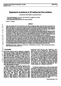
4 Noise reduction by increasing the signal-to-noise ratio (SNR) As explained above, acoustic measurements based on the Doppler principle require the scattering of acoustic waves on acoustic targets moving with the fluid. Shen and Lemmin (1997) have shown that the acoustic targets for the ADVP are turbulence induced air bubble microstructures with a mean size of about 750 µm, which are ideal flow tracers since they follow the fluid motion with negligible inertial lag. The size of the ideal flow tracers depends on the frequency of the emitted acoustic wave and is thus instrument dependent. Most commercial ADV instruments operate at a higher frequency than our ADVP, which emits1 MHz-pulses, and require smaller targets.

I.29 ADV instruments are known to perform poorly in (very) clear water characterized by a low acoustic scattering level, as is often found in laboratory applications or in naturally clean water areas such as the deep ocean, deep lakes, arctic water, etc. The successful application of ADV measurements in such cases requires an artificial supply of neutral acoustic targets to the water in order to increase the SNR. Note that this is particularly important for three-receiver ADV configurations where no accurate noise reduction techniques can be applied. The aim of this section is to describe a simple, low cost, nonpolluting technique of supplying acoustic targets to the water that has proven to be successful in measurements with the ADVP and with a commercial Nortek NDV (not shown). The technique, illustrated in Fig. 10, consists of generating hydrogen bubbles of the correct size in the fluid by means of electrolysis. The cathodic and anodic electrodes are formed by an array of horizontal stainless steel wires with a diameter of 100 µm that cover the entire water depth with a vertical spacing of about 1 cm. The spacing between the two electrodes is about 2cm and they are placed about 15cm upstream of the measured vertical water column. This distance is about 1500 times the wire diameter, which is sufficient to avoid any perturbation in the turbulence characteristics. The horizontal span of both electrodes has to be adequate to assure that the measured water column is outside the wake of the vertical insulating stems which carry the wires. A constant tension of O(5V) was sufficient to obtain a high acoustic scattering level with this configuration. The bubble generation is initially not efficient when the stainless steel wires are still clean. After some minutes, a surface reaction takes place on the wires and the bubble generation becomes efficient. Note that a similar supply of hydrogen bubbles to the flow has been commonly used in the past to measure velocities by means of the socalled hydrogen bubble technique. ADVP: see Fig. 5 hydrogen bubble generation +: anode - : cathode water surface

+

_

R2,R3

emitter

αi

R1, R4

αi

1[cm] flow

bottom insulating stem stainless steel wire 100µ >15[cm]=1500 x wire diameter large enough to have the measured water column outside the wake of the vertical stems

Fig. 10: Application of acoustic target supply by hydrogen bubble generation

I.30 The measurements with the optimized four-receiver ADVP configuration presented in the previous section were carried out with a supply of acoustic targets by this technique. They will now be compared to measurements without bubble injection under identical flow conditions (both treated with NPP=16 corresponding to fN= 31.25 HZ).

′2 and v˜x′ 1v˜x′ 2 , Vertical profiles of the longitudinal turbulent normal stress, estimated as v˜x1 are shown in Fig. 11. They indicate that the measurements with a low acoustic scattering level contain considerably more noise. Even the estimate of v˜x′ 1v˜x′ 2 , which in theory should be noise free, still contains a rather important noise contribution. The noise correction methods presented and illustrated in the previous section thus require a sufficiently high SNR. Note that the turbulence results should be independent of the acoustic scattering level under the condition that it is sufficiently high. 1

0.8

}

perturbation due to ADVP housing touching the surface a low acoustic scattering level b

0.6

high acoustic scattering level

2a 1b

z/H

1

′2 u∗2 v˜x1

2

′ v˜x2 ′ u∗2 v˜x1

2b

0.4

1a

0.2 0 0

4

v˜x′ 2 u∗2

12

16

20

Fig. 11: Estimates of longitudinal turbulent normal stress with low and high acoustic scattering level

[ /]

1.5

0 2a b 1

-2

3

10 -1

2b low acoustic scatter level high acoustic scatter level (bold)

b 1

6

2

′2 u∗2 v˜x1 ′ v˜x2 ′ u∗2 v˜x1

1a

4.1 4

0

a -1

2

10

1b

3b

8

2.3

2a

′2 u∗2 v˜x1 ′ v˜x2 ′ u∗2 v˜x1 2 σ x1 u∗2

2b

2 1b

10 0

f [Hz]

10 1

10 2

9.7

low acoustic scatter level high acoustic scatter level

0 10 -1

10 0

f [Hz]

10 1

f N = 31 25

10

5

3a

ij

10

1a

b a

f

2 Sij u* [Hz-1 ]

10 1

10

2 *

a

∫ S ( f´ )df´ u

10 2

f N = 31 25

′2 and v˜x′ 1v˜x′ 2 , for the level The corresponding (co)spectra and cumulative (co)spectra of v˜x1 ′2 in the measurements at z/H=0.4, confirm these findings. The noise contribution to v˜x1 with a low acoustic scattering level is higher than in those with a supply of acoustic targets. In both cases it remains nearly constant over the frequency range. The cospectrum and cumulative cospectrum of v˜x′ 1v˜x′ 2 for the measurements with a supply of acoustic targets show the typical –5/3-slope and “S” shape, respectively, and appear to be of good quality. Their counterparts for the measurements with low acoustic scattering level indicate that the remaining noise in v˜x′ 1v˜x′ 2 mainly affects the frequency range above 1 Hz.

10 2

′2 , Fig. 12: Normalized power (co)spectra (a) and cumulative power (co) spectra (b) of v˜x1 2 v˜x′ 1v˜x′ 2 and σ x,1 for high and low acoustic scattering level

I.31 Even though the measurements with low acoustic scattering level yield low quality turbulence results that are polluted by noise, they still give good estimates of the timeaveraged velocities, as shown in Fig. 13. Nearly identical profiles of the time-averaged longitudinal velocity are obtained for low and high acoustic scattering levels. This confirms that the noise is unbiased, σ i = 0 . Hence it does not affect the estimates of the time-averaged velocity.

perturbation due to ADVP housing touching the surface

0.8

0.6

z/H 0.4

}

1

v˜x1 U and v˜x2 U measured with low and high acoustic scatter level of the fluid

0.2 0

0

0.2

0.4

v˜x U

1

1.2

1.4

Fig. 13: v˜x1 U and v˜x2 U measured with low and high acoustic scattering level It can be concluded that accurate measurements of the time-averaged velocities can be obtained even with low acoustic scattering levels, but that accurate turbulence measurements require a high acoustic scattering level which can be improved by supplying suitable acoustic targets to the flow.

5 Conclusions This paper proposes efficient ways to reduce the parasitical noise contribution in pulse-topulse coherent Acoustic Doppler Velocimetry (ADV) thereby improving turbulence measurements with such instruments. Although the three-dimensional mean flow field can be accurately measured with three-receiver ADV instruments, turbulence measurements with these instruments suffer from parasitical noise contributions that cannot be accurately estimated and eliminated. To overcome this problem, Hurther and Lemmin (2001) propose the HL method, based on an ADV configuration with four instead of three receivers. Due to the fourth receiver, a redundancy of the vertical velocity component exists that allows to estimate the noise level and subsequently extract it from the longitudinal and transversal velocity components. In the present investigation, this four-receiver ADV system has been optimized by turning the receiver plains by 45° with respect to the direction of the mean flow. This reorientation has several advantages:

I.32 -

It provides for redundant information on all three velocity components which theoretically allows to directly obtain all turbulent stresses free of noise. This avoids the potential of error propagation which may result from the application of the HL method.

-

The quality of the measurements can be checked with this configuration because the noise levels of all three velocity components can be directly estimated from the measurements. Furthermore, from this information the noise level of each receiver can be individually determined providing a continuous check on the performance of the instrument. This is a great advantage over the previous fourreceiver ADVP which did not allow this detailed system check.

The parasitical noise is not completely eliminated by the proposed method. It is, however, reduced by about an order of magnitude when compared to the uncorrected results where the uncorrected results represent the level that can be obtained with three-receiver instruments. Therefore, the useful frequency range characterized by low noise levels is also extended by about an order of magnitude. The knowledge of the noise levels through the calculation of noise spectra allows to estimate the accuracy of the turbulence measurements. We have demonstrated that cumulative power spectra are particularly well suited for the determination of the noise effects and their elimination due to their particular shape in turbulent flow. They allow: -

to investigate the quality of the data. Power spectra become always noisy at the high frequency end and the amplitude of the variation makes it often difficult to determine the mean spectral slope in that range (Fig. 8a). Cumulative power spectra are smooth and therefore indicate more clearly the trend at the high frequency end (Fig. 8b). We have demonstrated that the noise effect strongly modifies this part of the cumulative spectra and this makes it easy to detect noise contributions.

-

to provide for an optimal choice of the measuring frequency. The presence of an inertial subrange in a power spectrum is in itself not yet a proof that the turbulence is well resolved in the measurements. The extent of the inertial subrange in the frequency domain depends on the specific flow conditions. Thus a cumulative spectrum should always reach past the “straight line” section and well into the high frequency curving part (Fig. 9). This is a good indication that a high enough sampling frequency has been chosen. However, it has to be realized that increasing the sampling frequency in an effort to extend the observations to higher frequencies may deteriorate the turbulence estimates. It risks to push the Nyquist frequency into a spectral region where only white noise is found (Fig. 9).

ADV instruments typically operate at a measuring frequency of O(20Hz). This may not always be sufficient to cover the full inertial subrange. It was demonstrated that turbulence is nearly isotropic above 10 Hz in the open-channel laboratory flow we have investigated. In this particular case the non-captured high frequency range does not significantly contribute to the turbulent normal stresses with the contribution being estimated at less than 10% (Fig. 9). This corresponds to the estimated system accuracy.

I.33 The contributions of the high frequency range to the turbulent shear stresses and the turbulent isotropy are even smaller. ADV instruments can thus resolve the low frequency part of the turbulence spectrum that interacts dynamically with the mean flow and that is important for the understanding of typical hydraulic processes. The non-captured, high frequency contribution mainly relates to the nearly-isotropic energy dissipation. ADV instruments can thus be successfully applied in many turbulence investigations provided that the noise contribution is correctly eliminated. However, in all these efforts it has to be remembered that the actual velocity sampling frequency is virtually restricted to what the acoustic targets can provide. Successful acoustic turbulence measurements with all ADV require sufficiently high acoustic scattering levels. Estimates of time-averaged velocities, on the other hand, are less sensitive and may still be possible at low acoustic scattering levels if measurements are taken over a sufficiently long time. Low scattering levels are often encountered in clear water, as is found in laboratory flumes, deep oceans, lake etc. Little can be done about this in a “natural” flow environment of deep oceans, lakes and some rivers. For laboratory studies, it is frequently suggested to “seed” the flow using small, almost neutrally buoyant particles as seeding material in order to increase the signal-to-noise ratio. Although this may be a solution in some cases, it is difficult, rather costly and may cause an undesirable pollution of the installation. A simple low cost and non-polluting technique to supply acoustic targets to the fluid has been described here which proved to be successful in our laboratory measurements. It consists of generating micro-hydrogen bubbles of an optimum size in the fluid by means of electrolysis. It is illustrated that very noisy turbulence measurements are obtained with low acoustic scattering levels and that a significant improvement in the quality of the results is possible by supplying sufficient micro-hydrogen bubbles as acoustic targets. The principal conclusion of this paper is that accurate turbulence measurements can be obtained with Acoustic Doppler Velocimeters by adopting an optimized four-receiver configuration of the instrument and by assuring a sufficiently high acoustic scattering level. Although uniquely illustrated by means of ADVP measurements which have the further advantage to allow non-intrusive profiling, the concepts outlined herewith can invariantly be applied to improve turbulence measurements with other ADV instruments.

Acknowledgements This research is being sponsored by the Swiss National Science Foundation under grants Nr.2100-052257.97/1 and 2000-059392.99/2. The first author gratefully acknowledges his PhD supervisor, Prof. W.H. Graf, for his support and Prof. H.J. de Vriend for many fruitful discussions during his stay at the EPFL.

I.34

APPENDIX I.

REFERENCES

Blanckaert, K. (2001). “Discussion on: Bend-flow simulation using 2D depth-averaged model.” J. Hydr. Eng.,127(2), 167-170. Blanckaert, K. & de Vriend, H. J. (2002). “Secondary flow in sharp open-channel bends.” (submitted for publication). Blanckaert, K. & Graf, W. H. (2001). “Experiments on flow in a strongly curved channel bend.” Proc. 29th IAHR Congress, Vol. D1, Beijing, China, 371-377. Cellino, M. & Graf, W. H. (1999). “Sediment-Laden flow in open-channels under noncapacity and capacity conditions.” J. Hydr. Eng, 125(5), 455-462. Garbini, J. L., Forster, F. K. & Jorgensen, J. E. (1982). “Measurement of fluid turbulence based on pulsed ultrasound techniques. Part I. Analysis.” J. Fluid Mech., 118, 445-470. Graf, W. H. & Yulistiyanto, B. (1998). “Experiments on flow around a cylinder; the velocity and vorticity fields.” J. Hydr. Res., IAHR, 36(4), 637-653. Graf, W. H. & Istiarto, I. (2002). “Flow pattern in the scour hole around a cylinder.” J. Hydr. Res., IAHR, 40(1), 13-20. Hurther, D. (2001). “Sediment transport assessment in suspension flow based on coherent structure characteristics.” Proc. JFK Student Paper Comp., 29th IAHR Congress, Beijing, China, 73-82. Hurther, D. & Lemmin, U. (1998). “A constant beamwidth transducer for threedimensional Doppler profile measurements in open channel flow.” Meas. Sciences Techn., 9(10), 1706-1714. Hurther, D. & Lemmin, U. (2001). “A correction method for turbulence measurements with a 3-D acoustic Doppler velocity profiler.” J. Atm. Oc. Techn., Vol.18, 446-458. Kolmogoroff, A. N. (1941). “The local structure of turbulence in incompressible viscous fluid for very large Reynolds numbers.” C. R. Acd. Sci. U.R.S.S., 30(301). Lemmin, U. & Rolland, T. (1997). “Acoustic velocity profiler for laboratory and field studies.” J. Hydr. Eng, 123(12), 1089-1098. Lhermitte, R. & Lemmin, U. (1994). “Open-channel flow and turbulence measurement by high-resolution Doppler sonar.” J. Atm. Oc. Techn., 11(5), 1295-1308. Nezu, I. & Nakagawa, H. (1993). Turbulence in open-channel flows, IAHR-monograph, Balkema. Nikora, V. (1999). “Origin of the "-1" Spectral law in wall-bounded turbulence.” Physical Review Letters, 83(4), 734-736. Rolland, T. (1994). “Développement d'une instrumentation Doppler ultrasonore adaptée à l'étude hydraulique de la turbulence dans les canaux.” PhD thesis no 1281, EPFL, Lausanne, Switzerland. Rolland, T. & Lemmin, U. (1997). “A two-component acoustic velocity profiler for use in turbulent open-channel flow.” J. Hydr. Res., 35(4), 545-561. Shen, C., & Lemmin, U. (1996). “A tristatic Doppler velocity profiler and its application to turbulent open-channel flow.” Advances in Turbulence VI, P. A. Monkewitz and S. Gavrilakis, eds., Kluwer Academic Publications, Lausanne, 483-486.

I.35 Shen, C. & Lemmin, U. (1997). “Ultrasonic scattering in highly turbulent clear water flow.” Ultrasonics, 35, 57-64. Shen, C. & Lemmin, U. (1998). "Anew method for probing the turbulence scalar spectrum by ultrasonic scanning." Experiments in Fluids, 24, 90-92. Song, T. & Graf, W. H. (1996). “Velocity and turbulence distribution in unsteady openchannels flows.” J. Hydr. Engng, ASCE, 122(3), 141-154. Song, T., Graf, W. H. & Lemmin, U. (1994). “Uniform flow in open channels with movable gravel bed.” J. Hydr. Res., ASCE, 32(6), 861-876. Tchen, C.M. (1953). "On the spectrum of energy in turbulent shear flow." J. Res. Natl. Bur. Stand., 50(1), 51-62. Voulgaris, G. & Trowbridge, J. H. (1998). “Evaluation of the Acoustic Doppler Velocimeter (ADV) for turbulence measurements.” J. Atm. Oc. Techn., 15, 272-289. Zedel, L., Hay, A. E., Cabrera, R. & Lohrmann, A. (1996). “Performance of a single beam pulse-to-pulse coherent Doppler profiler.” J. Oceanic Eng., IEEE, 21(3), 290297.

APPENDIX II.

NOTATION

ADV ADVP B Fr= U / gH H Lx NPP Q Re=UH/ν Sb Sij SNR Tx U c f k prf vj x,y,z

= = = = = = = = = = = = = = = = = = = =

Acoustic Doppler Velocimeter / Velocimetry Acoustic Doppler Velocity Profiler flume width Froude number flow depth macro lengthscale of turbulence in the wavenumber space number of pulse-pairs discharge Reynolds number of reach-averaged flow downstream bottom slope cospectrum of components i and j signal-to-noise ratio macro timescale of turbulence in the frequency space Q/(BH) = globally-averaged velocity speed of sound in the fluid frequency wavenumber pulse-repetition-frequency velocity component along i-direction longitudinal, transversal and vertical reference axes

symbols α β λ ν σ arrow

= = = = = =

angle between vertical and scattered wave angle between longitudinal axis and vertical (emitter-receiver) plane wavelength molecular viscosity of water; ν= 1.004 x 10-6 m2/s at 20° noise contribution on a receiver or a velocity component vector quantity

I.36 overbar prime tilde O(.) subscripts D H HL N e r

= = = =

= = = = = =

time-averaged values fluctuating part of a quantity (with zero time-averaged value) measured value of a quantity that estimates its true value order of magnitude of .

Doppler horizontal component or projection in the horizontal (x,y)-plane reference to Hurther and Lemmin (2001) Nyquist emitter receiver

PART II EXPERIMENTAL OBSERVATIONS II.0 Introduction II.1 Mean Flow and Turbulence in Open-Channel Bend II.1 II.2 Bend-Flow Simulation Using 2D Depth-Averaged Model II.15 II.3 Experiments on Flow in a Strongly Curved Channel Bend II.19 II.4 Secondary Currents Measured in Sharp Open-Channel Bends II.27 II.5 Conclusions II.37 ________________________________________________________________________

II.0

Introduction

An Acoustic Doppler Velocity Profiler (ADVP), developed in our laboratory, has been used to measure in detail the three-dimensional flow field and the turbulence in openchannel bends. A limited series of experiments in a small low-budget flume, done with the aim of testing the capabilities of the ADVP, was followed by extended series of experiments in a large optimized flume. This dissertation mainly considers the smallflume experiments, which yielded results beyond all expectations, and only includes few large-flume results. This part II presents the most relevant experimental data and observations that are subsequently analyzed in parts III and IV. It consists of four papers with the following contents: - chapter II.1 explains the working principle of the ADVP and the data-analysis techniques. Furthermore, it presents distributions of all three mean velocity components and all six Reynolds stresses as well as the mean flow and turbulent kinetic energy measured in the small-flume experiments. - chapter II.2 compares distributions of the downstream velocity and the secondary circulation measured in the small-flume experiments with predictions according to linear models, which are commonly used to account for the vertical dimension of the flow field in depth-integrated flow models. Chapter IV.1 will explain these linear models in detail. - Similar to the previous paper, chapter II.3 compares distributions of the downstream velocity and the secondary circulation measured in the large-flume experiments with linear model predictions. - chapter II.4 presents three-dimensional patterns of the downstream velocity and the multi-cellular secondary circulation measured in the large-flume experiments. At the end of Part II, the main conclusions are summarized. Some other small-flume data have been presented in a paper that is not included in this dissertation: Blanckaert, K., and Graf, W. H. (1999) “Experiments on flow in open-channel bends.” Proc. 28th congr. IAHR., Techn. Univ.Graz, Graz, Austria, CD-ROM.

II.1

II.1

MEAN FLOW

AND

TURBULENCE

IN

OPEN-CHANNEL BEND

By Koen Blanckaert1 and Walter H. Graf,2 Member, ASCE ABSTRACT: Flow over a developed bottom topography in a bend has been investigated experimentally. The measuring section is in the outer-bank half of the cross section at 60⬚ into the bend. Spatial distributions of the mean velocities, turbulent stresses, and mean-flow and turbulent kinetic energy are presented. The cross-sectional motion contains two cells of circulation: besides the classical helical motion (center-region cell), a weaker counterrotating cell (outer-bank cell) is observed in the corner formed by the outer bank and the water surface. The downstream velocity in the outer half-section is higher than the one in straight uniform flow; the core of maximum velocities is found close to the separation between both circulation cells, well below the water surface. The turbulence structure in a bend is different from that in a straight flow, most notably in a reduction of the turbulent activity toward the outer bank. Both the outer-bank cell and reduced turbulent activity have a protective effect on the outer bank and the adjacent bottom and thus influence the stability of the flow perimeter and the bend morphology.

INTRODUCTION Most natural rivers meander and tend to erode the outer banks in their successive bends. Important engineering efforts are undertaken on rivers of all scales to stabilize the banklines. This is an essential component of projects to improve navigability; increase flood capacity and decrease floodplain destruction; avoid massive loss of fertile soil (Odgaard 1984); and reduce dredging requirements of the river. Recently, there has been an increased interest in the modeling of the erosional behavior of the outer bank (see the discussion section). However, little is known about the characteristics of the mean flow and turbulence near the outer bank, where the flow pattern is highly three-dimensional (3D). A large amount of research on flow in bends has been performed in the last decades, but most of the experimental investigations concentrated on the central portion of the flow and often did not cover the outer-bank region in detail. Moreover, in most investigations a fixed rectangular section with a smooth bed was imposed on the flow. This is different from the rough turbulent flow over a typical developed bed topography, as found in nature. Furthermore, in most experimental investigations, not all of the three velocity and six turbulent stress components were measured, and the measuring grids were rather coarse. A literature review of experimental research on flow in open-channel bends is given in Table 1. More recently, environmental problems such as the spreading and mixing of pollutants or the transport in suspension of polluted sediments have become of major concern in river management. These phenomena are closely related to the turbulence structure of the flow. The scarcity of reliable experimental data on the 3D flow pattern and turbulence structure, particularly in bends, is responsible for the lack of insight into the physical mechanisms, such as those related to outer-bank erosion and the mixing of pollutants. Furthermore, this lack hampers the verification of investigations by means of numerical simulations. In this study, detailed measurements were made of a rough turbulent flow in equilibrium with its developed bottom topography. Special attention was given to the complex flow 1 Res. Assoc., Lab. de Recherches Hydrauliques, Ecole Polytechnique Fe´de´rale, CH-1015 Lausanne, Switzerland. 2 Prof., Lab. de Recherches Hydrauliques, Ecole Polytechnique Fe´de´rale, CH-1015 Lausanne, Switzerland. Note. Discussion open until March 1, 2002. To extend the closing date one month, a written request must be filed with the ASCE Manager of Journals. The manuscript for this paper was submitted for review and possible publication on April 4, 2000; revised May 16, 2001. This paper is part of the Journal of Hydraulic Engineering, Vol. 127, No. 10, October, 2001. 䉷ASCE, ISSN 0733-9429/01/0010-0835–0847/$8.00 ⫹ $.50 per page. Paper No. 22307.

region near the fixed vertical outer bank. Nonintrusive measurements were made on a fine grid with an acoustic Doppler velocity profiler (ADVP), which simultaneously measures instantaneous profiles of all velocity components. This enables one to evaluate the three mean velocity components, vj ( j = s, n, z), along the downstream, transversal, and vertical axes, respectively [Figs. 1 (a and c)], as well as the six turbulent ⬘ ( j, k = s, n, z). stress components, ⫺␳v ⬘v j k This paper aims at improving our understanding of the flow and turbulence in bends and their relationship to boundary erosion and spreading (mixing) of pollutants. Furthermore, due to the detailed measurements on a fine grid, we want to provide a useful data set for verification of numerical simulations of the flow field. The paper gives a description of the experimental facility, hydraulic parameters, ADVP, and data-treatment procedures. Spatial distributions of the mean downstream velocity, mean cross-sectional motion, turbulent normal and shear stresses, and mean-flow and turbulent kinetic energy are presented and analyzed. The importance of the observed flow and turbulence distributions with respect to the stability of the outer bank and the adjacent bottom are discussed. EXPERIMENTAL INSTALLATION Experiments were performed in a B = 0.4 m wide laboratory flume with fixed vertical sidewalls made of plexiglass, consisting of a 2 m long straight approach section followed by a 120⬚ bend with a constant radius of curvature of R = ⫺2 m [Fig. 1(a); R is negative along the n-axis]. Initially, a horizontal bottom of nearly uniform sand, d50 = 2.1 mm, was installed. Subsequently, a discharge corresponding to clear-water scour conditions was established. As a result, the bottom in the straight approach channel remained stable, but a typical barpool bottom topography developed in the bend. Ultimately, this topography stabilized and there was no active sediment transport along the flume. The resulting developed bottom topography is shown in Fig. 1(a). The transversal bottom slope increases from ⬃0⬚ at the bend entry to a maximum value of ⬃24⬚ at 45⬚ into the bend and subsequently shows an oscillating behavior [Fig. 1(b)]. A number of analytical models for the flow and the bottom topography have been proposed that qualitatively predict such a behavior (de Vriend and Struiksma 1984; Odgaard 1986). A comparison of different models can be found in Parker and Johannesson (1989). A superelevation of the water surface [Fig. 1(b)] develops from the bend entry onto ⬃45⬚ into the bend. Subsequently it remains nearly constant (the fluctuations are within the measuring accurace) at ⬃0.65⬚, yielding a difference of ⌬zs = 4.5 mm = 1.5(B/R)(U 2/g) in water surface elevation between the two banks. The hydraulic conditions of the flow over this bottom toJOURNAL OF HYDRAULIC ENGINEERING / OCTOBER 2001 / 835

II.2 TABLE 1.

Literature

Literature Review of Experimental Research on Flow in Open-Channel Bends

Cross section and channel bed

Planform

Flow regime

Size of measuring grid (approximately)

Number of vertical profiles in outerbank region

Flow and turbulence measurements

Rozovskii (1957)

Rectangular: smooth bed rough bed Triangular

Single bend, 180⬚

Transition Rough turbulent Transition

H/7 ⫻ B/8 H/7 ⫻ B/8 H/7 ⫻ B/4

2 2 1

vs , vn

Go¨tz (1975)

Rectangular smooth bed

Single bend, 180⬚

Transition

H/5 ⫻ B/10 (denser near banks and bottom)

2, 3, 4, 5 (for aspect ratios of 20, 10, 4.6, 2.9)

vs , vn

de Vriend (1979)

Rectangular smooth bed

Single bend, 180⬚

Transition

H/10 ⫻ B/10

3

vs , vn

de Vriend (1981)

Rectangular rough bed

Single bend, 180⬚

Rough turbulent

H/10 ⫻ B/10

3

vs , vn

Siebert (1982)

Rectangular smooth bed

Single bend, 180⬚

Transition

H/5 ⫻ B/4 z/H = 0.09, 0.66 ⫻ B/3

3 2

vs , vn vz , v⬘v⬘ j k

Dietrich and Smith (1983)

Natural topography; sand bottom

Meander, field study

Rough turbulent

H/6 ⫻ B/13

0, resulting—due to continuity— in a much too large downflow, w ¯ < 0, concentrated in a thin layer near the outer bank [Figs. 18 and 19(c)]. Dispersion stresses based on such an unrealistic pattern of secondary flow cannot be expected to model correctly the transversal momentum convection and will notably fail to account correctly for the influence of the impervious banks. Ikeda et al. (1990) have presented analytical solutions for u¯ and v¯ that are valid over the whole cross section, including the bank boundary layers. Dispersion terms based on their profiles should model more correctly the transversal momentum convection and the influence of the impervious banks. The authors have tested their model for two cases. The first concerns a mildly curved flow, R c /B = 8.3, for which de JOURNAL OF HYDRAULIC ENGINEERING / FEBRUARY 2001 / 169

II.18 Vriend’s assumptions seem to be justified. The second case concerns a strongly curved flow, R c /B = 1, in which the dispersion stresses contribute significantly to the momentum balance. The discusser’s experimental data show that the authors’s model of momentum convection by dispersion stresses is unreliable for strong curvatures. Our measured flow field is highly three-dimensional, as shown by the important interaction between the streamwise velocity and the secondary flow and by the appearance of an outer-bank cell of circulation [Figs. 18(b and c)]. In the discusser’s opinion, only fully 3D simulations can be reliable for strongly curved flows. Unfortunately, no channel bends with a curvature of R c /B ⬃ 3, which is typical for natural bends, were tested by the authors. The above remarks and our experimental result are aimed to show that care should be taken when applying the authors’ model to bends of moderate or strong curvature.

170 / JOURNAL OF HYDRAULIC ENGINEERING / FEBRUARY 2001

APPENDIX.

REFERENCES

Blanckaert, K., and Graf, W. H. (1999). ‘‘Outer-bank cell of secondary circulation and boundary shear stress in open-channel bends.’’ RCEM Symp., Vol. 1, Genova, Italy, 533–543. de Vriend, H. J. (1981a). ‘‘Velocity redistribution in curved rectangular channels.’’ J. Fluid Mech., 107, 423–439. de Vriend, H. J. (1981b). ‘‘Steady flow in shallow channel bends.’’ Rep. No. 81-3, Dept. of Civ. Engrg., Delft University of Technology, Delft, The Netherlands. Ikeda, S., Yamasaka, M., and Kennedy, J. F. (1990). ‘‘Three-dimensional fully developed shallow-water flow in mildly curved bends.’’ Fluid dynamics research 6, North-Holland, 155–173. Johannesson, H., and Parker, G. (1989). ‘‘Velocity redistribution in meandering rivers.’’ J. Hydr. Engrg., ASCE, 115(8), 1019–1039. Yulistiyanto, B., Zech, Y., and Graf, W. H. (1998). ‘‘Free-surface flow around cylinder: shallow-water modeling with diffusion-dispersion.’’ J. Hydr. Engrg., ASCE, 124(4), 419–429.

II.19

II.3

Experiments on Flow in a Strongly Curved Channel Bend K. BLANCKAERT and W.H. GRAF Proceedings XXIX IAHR congress, Theme D, Vol. I, 371-377, Beijing, China, Sept 2001

ABSTRACT The secondary circulation in open-channel bends largely determines the bed topography. It is often described by the “Rozovskii model” in depth-integrated flow models. Our experimental results indicate that the “Rozovskii model” has a tendency to overpredict the strength of the secondary circulation and its effect on the velocity distribution for the case of strongly curved open-channel flow. Both also decrease with increasing curvature ratio; this is in contrast with the unique dependence on the Chezy coefficient predicted by the “Rozovskii model”. KEYWORDS strongly curved flow, open-channel bend, secondary circulation, experiments INTRODUCTION The most characteristic feature of curved flow is the helical flow pattern, also known as secondary circulation. It advects flow momentum and redistributes transversally the velocity and the boundary shear stress over the bend. Furthermore, the direction of the bottom shear stress, and thus also of the sediment transport, directly depends on the strength of the secondary circulation. As a consequence, the evolution of the secondary circulation will largely determine the resulting bed topography with its characteristic bar-pool formation. Since fully-3D flow models are not yet feasible for engineering problems concerned with the river morphology, most often 2D depth-integrated flow models are used. By depth-integrating the flow equations, all information on the secondary circulation is lost. However, as mentioned above, it is essential to account for the effect of the secondary circulation and this can only be done by providing it as input to the model. This input is mostly based on simplified expressions for the velocity profiles, which have been proposed by Rozovskii (1957). In this paper, experimental data is presented that illustrates the shortcomings of this approach for strongly curved flows. Blanckaert (2001) presents a model for the velocity profiles in strongly curved flows that explains the features observed in the here reported experiments. THEORETICAL CONSIDERATIONS The distribution of the depth-averaged downstream velocity, Us, is governed by the depthintegrated downstream momentum equation. Assuming a hydrostatic pressure, this equation is (Dietrich and Whiting, 1989):  1 ∂ 1 2 v sv n h  τ bs ∂z ∂ = − gh S −  v 2s h + v sv n h +  1 + nR 1 + n R R  ρ ∂s ∂n 1 + n R ∂s G C1 C2 C3 τ ρ h 2 ∂ ns + τ ns ρ h + (1) n 1+ R ∂n R T1 T2

(

(

)

)

(

)

II.20

where τbs is the downstream component of the bottom shear stress, ρ is the water density, g is the gravitational acceleration, h is the local flow depth, R is the centreline radius of curvature, (1+n/R) is a metric factor, zS is the elevation of the water surface above the horizontal reference plane (s,n) (for which the flume-average bottom level is chosen), τ ns is a component of the Reynolds tensor and vj (j=s,n,z) are the time-averaged velocity components along the reference axes. The s-axis follows the channel centreline, the n-axis is perpendicular to it and points towards the outer bank and the vertical z-axis is positive in upward direction (Fig.1a). The , indicate depth-averaged values. brackets, In a 2D straight uniform flow, the bottom shear stress τbs/ρ is in equilibrium with the energy expenditure G in all points (s,n) of the flume, and the momentum equation reduces to τbs/ρ=G. In a 3D flow, the velocities are non-uniformly distributed and the other terms have to be considered. The terms T1 and T2 are shear stresses which are mainly generated by transversal velocity gradients; they are usually of minor importance. The terms C1, C2 and C3 represent advective transport of momentum. C1 is due to downstream variation of the flow field and drops out when the flow is completely adapted to the curvature (∂/∂s=0). The non-uniform velocity distribution over the channel width is mainly due to the terms C2 and C3. These are redistribution terms that nearly cancel when integrated over the cross-section. They represent the effect of the advective transport of downstream momentum, ρvs, by the transversal velocities, vn, which after depthintegration yields: ρh v sv n . By decomposing the velocity components vj (j=s,n) in a depthaveraged value, v j =Uj, and its local deviations, v∗j : v j = v j + v ∗j = U j + v ∗j

v ∗j = 0

where

(2)

the velocity redistribution term can be decomposed as:

(

)(

v sv n = Us + v ∗s Un + v ∗n

)

= UsUn + v ∗s v ∗n

(3)

The first term, UsUn, represents a redistribution of downstream velocity Us by the transversal velocity Un; it can be resolved by depth-integrated flow models. The second term, v ∗s v ∗n , represents the velocity redistribution by the secondary flow; since it depends on the vertical distributions of v∗s and v∗n , it is an unknown in the depth-integrated momentum equation and has to be modelled. Often, this term is modelled using vertical profiles of v∗s and v∗n that are derived from a simplified set of the 3D Navier-Stokes equations, proposed by Rozovskii (1957). de Vriend (1977) gives the following solution of these simplified equations, which will be called the “Rozovskii model” further on:

(

)

v ∗s = v s − Us = Us f s − 1 = v ∗n = Us

Us

(

)

g 1 + ln η κC

η η   g ln 2 η′ g h h 1  ln η′  η f n = − Us 2 d + dη′ + 1 − f s ( η)  ′  ∫ ∫ 2 κC η 0 1 − η′ κC  R R κ  η 0 1 − η′   

(4)

(5)

II.21

where fs and fn are the normalised profiles of vs, and vn*, C is the Chezy friction coefficient, κ is the von Karman constant, η=z/h is the normalised vertical co-ordinate and η0 is the near-bottom level where fs(η0)=0. According to the “Rozovskii model”, the secondary circulation, v∗n , increases linearly with increasing curvature ratio, h/R, for a given downstream velocity, Us. fs fn represents the velocity redistribution term v∗s v∗n normalised by Us2h/R:

(

)

v ∗s v ∗n = v s − Us v ∗n = U2s

(

)

h h f s − 1 f n = U2s f sf n R R

(6)

where fn = 0. fs fn is called the velocity-redistribution coefficient further on, while fn2 shall be interpreted as the normalised strength of the secondary circulation. According to the expressions, eq.4 and eq.5, both fs and fn, - and thus also fn2 and fs fn - are unique functions of the Chezy friction coefficient, C, and do not depend on the curvature parameter, h/R. fn2 and fs fn calculated from the “Rozovskii model” as a function of C are shown in Fig.3. In this paper, predictions of fn2 and fs fn based on “Rozovskii model” (eq.4 and eq.5 and shown in Fig.3) will be compared with experimental data for a strongly curved open-channel bend (Fig4 and Fig.5). The experimental normalised velocity profiles are calculated from the measured distributions of vs(η) and vn(η) according to eq.2, eq4 and eq.5 as: f s η = vs η U s (7)

() () (η) = v (η)

 H  H (8)  U s  = v n η − Un  U s   R  R where the flume-averaged water depth, H, will be used as an approximation for the local water depth, h. fn

∗ n

( ()

)

THE EXPERIMENTS (FIG.1) Experiments were performed in a 1.3m wide laboratory flume, consisting of a 9m long straight inflow, followed by a 193° bend with a constant radius of curvature of R=1.7m on the centreline, and a 5m long straight outflow. The horizontal bed was covered by a sand with diameters in the range 1.6mm < d < 2.2mm, which has been fixed by spraying a layer of paint on it, thus preserving the roughness of the sediments. The vertical banks were made of Plexiglas. A ratio R/B=1.31 was chosen, which corresponds to a very strongly curved bend; a bend is considered strongly curved when R/B0 and that all kinetic energy fluxes are definitely positive:

III.40 2 + ezz2 + 2 esn2 + 2 esz2 + 2 enz2 ) >0 P= 2ν t (ess2 + enn

(16)

This implies that kinetic energy is always transferred from the mean flow to the turbulence. By implication, when using a linear eddy viscosity concept the cross-stream turbulence terms in the downstream vorticity equation (4) are always dissipative. This means that this concept is not applicable to flows in which turbulence somehow contributes to the mean kinetic energy.

3 Present objectives From the above review of the current state of knowledge it can be concluded that the mechanisms underlying the centre-region cell and the outer-bank cell are not yet fully understood. Research so far was mostly restricted to the downstream vorticity equation. Here we will carry out a simultaneous analysis of the downstream vorticity dynamics (cf. equations (4/6) and figure 6) and the kinetic energy transfer between mean flow and turbulence (cf. equation (11) and figures 7-8). This analysis will be based on the data resulting from the experiment described hereafter. It will concern the following questions: •

What are the relevant mechanisms behind the generation of the centre-region cell? Does the simplified vorticity equation (8), which is often used to model the centreregion cell, capture all relevant mechanisms? What are the roles of advective transport and turbulence?

•

Can the hypothesis of de Vriend (1981a) and Christensen et al. (1999) that the outerbank cell formation is associated with both skewing-induced and turbulence-induced vorticity be confirmed or rejected? What is the interaction between the two mechanisms?

•

What is the role of the cross-stream turbulence terms, v n′2 - v z′2 and v n′ v z′ , in the generation of turbulence-induced vorticity? The availability of data on all turbulent stress components must enable investigating this role in further depth.

•

To what extent does the cross-stream turbulence dissipate or generate vorticity? A simultaneous analysis of the downstream vorticity dynamics and the transfer of kinetic energy between mean flow and turbulence must give further insight at this point.

•

What aspects are essential to the numerical modelling of strongly curved openchannel flow, and especially of the outer-bank cell?

Furthermore, this paper presents a detailed data set on strongly curved turbulent flow with a double pattern of cross-stream circulation cells.

III.41

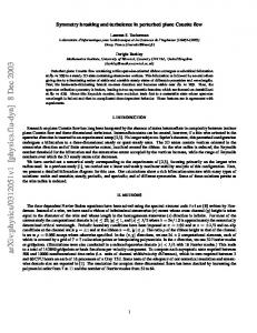
4 Analysis of experimental data 4.1 The experiment A separate paper (Blanckaert & Graf 2001a) has been dedicated to the presentation of the experimental set-up, the instrumentation, the measuring grids, the estimation of the experimental accuracy, the data treatment procedures and the distributions of the mean velocity components and the turbulent stress components. Here only features that are of particular relevance to the present analysis are repeated. Flow measurements were performed in a laboratory flume of 0.4 m wide, consisting of a 2 m long straight approach reach, followed by a 120° bend to the left of constant curvature (radius 2 m). The initially horizontal sand bottom was deformed by the flow, via a process of so-called clear-water scour. Ultimately, the sediment transport vanished throughout and a bottom topography in static equilibrium with the flow was obtained (figure 3). pool -7 -6

Figure 3(a)

-5 -3 -1 0 1 2 3

90°

n

-4

R2

4

pool 60°

120

°

outlet basin

R4 -5

z s

ADVP: central emitter surrounded by four receivers, R1 to R4, placed in water-filled box attached to bank

reference system - (s-n): horizontal - z : vertical

-6

6 point bar

-5 -4 -3 -2

5 4 3

30°

2

bottom levels [cm] indicated with respect to reach-averaged bottom level

-1

1

0

0 0 R=-2m

CL 2.6

H=11.4

point bar

h

B/2 -1 d50

Figure 3(b) investigated cross-section at 60° B=040 scales in [cm] CL zS

d50=0.21

0°

(R v z′2 . In the region near the outer bank, the transversal fluctuations are hindered and v n′2 < v z′2 . The damping of the fluctuations by the water surface is only slightly weaker than that by the outer bank, and the line where v n′2 = v z′2 , drawn in figure 5(a), only slightly deviates from the bisector of the upper right corner of the flow domain. There, the pattern of v n′2 - v z′2 is nearly antisymmetrical about this line. Similar patterns of v n′2 - v z′2 have been observed in experiments with straight uniform flow (Nezu et al. 1985, for airflow in a duct, Tominaga et al. 1989, for open-channel flow). Nezu & Nakayama (1998, 1999) have shown that the damping by the water surface depends on the Froude number. For low Froude numbers, like in the present experiment, the water surface almost completely dampens the nearby vertical fluctuations, whereas this damping gets less as the Froude number increases.

45°

CL control volume shown in figure 2(b) 0.25 0.2 0.15 0.08 0.05

-0.6 -0.5

0.03 -0.4

-0.3

-0.2

-0.1

-0.05

extrapolation: v n′ v z′ =0 at the water surface

outer-bank region

0 0.01

-0.5 -0.6

0

outer bank

centre-region

45°

-0.3 -0.4 -0.2 -0.1 -0.05

45° 0.02

-0.18

-0.16

-0.14 -0.12

0.03 1

0.05

z

-0.14 -0.12 -0.1 -0.08 -0.06 -0.05 -0.06 -0.08 -0.1 -0.04 -0.02 0 0.02

s

n 20 [cm] 18

(v ′

2 n

16

− v z′2 14

) 12

z

s

n

10

8

6

4

2

0

0.03 0.02 0

0.8 0.6 0.4 0.2 0.05

u∗2,60

45°

0 -0.02 -0.04

20 [cm] 18

0

−v n′ v z′ u∗2,60 16

14

12

10

8

6

(

4

Figure 5: Isolines of normalized (a) turbulent normal stress difference, v n′2 − v z′2 (b) turbulent shear stress, −v n′ v z′ u∗2,60 .

2

)

0

u∗2,60 ;

The turbulent shear stress v n′ v z′ seems to be correlated with the circulation cells. Even though the cells have a different sense of rotation, this turbulent shear stress does not change sign. Near the ‘eye’ of the weaker outer-bank cell, the absolute value is only slightly less than near the ‘eye’ of the centre-region cell. The pattern of v n′ v z′ is nearly symmetrical about the bisector of the upper right corner of the flow domain, which again indicates a similar influence of the water surface and the outer bank on the turbulent stresses. A similar near-corner pattern of v n′ v z′ has been measured by Nezu & Nakagawa (1984) in the case of air-flow in a duct. It is to be expected that the influence of the water surface on v n′ v z′ also depends on the Froude number. In the region dominated by bottom friction, this stress component is primarily associated with the transversal component of the bottom shear stress. It is positive there, since the bottom shear stress is directed towards the centre of curvature, so in the positive n-direction.

III.46

4.3 Analysis of the centre-region cell 4.3.1

Observations (Figures 4(e), 6 and 7)

As mentioned before, there is an important feedback between the downstream velocity and the centre-region cell. Skewing of existing mean vorticity by the centrifugal force, –vs2/R, is the principal generation mechanism of the centre-region cell. Integrated over the water depth, the centrifugal term in the vorticity equation (4/6) is always positive, which complies with the sense of rotation of the centre-region cell. In curved flow, advective momentum transport by the centre-region cell deforms the vertical v s-profiles by decreasing vs in the upper part of the water column and increasing it in the lower part. This is why the velocity maximum in the present experiments is found in the lower part of the water column (figure 4(c)). As a consequence, the centrifugal term –(∂/∂z)(vs2/R) in the vorticity equation is negative in a significant part of the water column (figure 6(a)), opposite to the observed sense of rotation of the centre-region cell. The advective transport terms in the vorticity equation, v n∂ωs/∂n+vz∂ωs/∂z, are of the same order of magnitude as the centrifugal term. They redistribute the vorticity over the cross-section. The positive values in the upper part of the water column (figure 6(b)) compensate for the negative centrifugal term (figure 6(a)). This explains why the centreregion cell extends over the entire water depth, instead of splitting into two cells on top of each other. The advective transport is generally dominated by the transversal contribution, vn∂ωs/∂n. The vertical contribution, which is not shown separately in figure 6, is usually much smaller. The role of the turbulent stress v n′ v z′ on the centre-region cell is complex. The v n′ v z′ -terms are of leading order in the vorticity equation (figure 6(d), cf. equation (8)). Close to the bottom, v n′ v z′ is associated with the transversal component of the bottom shear stress. Hence, the v n′ v z′ -term in the vorticity equation opposes the observed vorticity in this layer, and mean-flow vorticity is dissipated into turbulence there (figure 7(b)). Just above that near-bottom layer, but still in the lower part of the water column, the v n′ v z′ -term favours the observed vorticity. Analysis of the energy equation shows that a weak kinetic energy flux from turbulence to the mean flow occurs via v n′ v z′ . In this zone, the centrifugal and v n′ v z′ -terms compliant with the existing vorticity are mainly balanced by the opposed advective transport term. As mentioned before, the turbulence measurements in the lower 20% of the water column are less accurate and should therefore be interpreted with care. In most of the upper part of the water column, the v n′ v z′ -term opposes the observed vorticity and mean-flow kinetic energy is transferred to turbulence. The v n′2 − v z′2 -terms in the vorticity equation are smaller than the other terms, but they are not negligible (cf. figure 6(c)). In the upper part of the water column, their sign is opposite to that of the observed (positive) vorticity. In the lower part of the water column, the sign of these terms complies with the observed vorticity.

III.47

CL

-0.6

outer bank

centre-region -0.2

-0.4 -0.5

1.75 2

-0.6

outer-bank region

1

0.5

0

-0.1

-0.8 -1 -1.2 -1.4 -1.5

0

0

1.75 1.5

-1

0 0

-1.1 -1.4

3 2.5 2

z

-1.3

-1.2

-1

-4

-3

-0.1

-1 -0.5

-2

1.5

s

z

0

1

s

0.5

0

n

n 20[cm] 18

16

14

12

10

8

6

4

2

20[cm] 18

0

16

14

12

10

8

6

4

2

0

extrapolation outside measuring grid based on v n′ v z′ ( z = zS ) = 0

-0.5 -0.4 -0.35 -0.3 -0.4 -0.2 -0.5

-0.1

-0.2 -0.3

0.5

0

-0.3

0

-0.1

0

0.1 0

-0.1 -2.5 3

0 0.2

-0.4 -0.5 -0.6 -2 -1.5 -0.8 -1

-0.2

-0.3

0

0

0.3

0.2

0.4 0.3

z

0.2

0

0.1 0.6

-0.2

0.4

2 1

0.1

0

0.4

0

z

s

0

0.2

-0.1

3 Hz have been filtered out, because they are considered to be parasitic (see below, Fig. 11a). Comparison with the normalized total shear stress shows that the width-coherent fluctuations have a relatively small contribution to the shear stress.

0.25 0.23 0.2

2 4

0.15 0.1

6

0.05

8 -1 -1.25 -1.4

-0.75

-0.5

-0.25 -0.1

0.03

0

10

0.05 0.1 0.15 0.2 0.23

12 -0.02

z

s

−v s′v n′ u

20 [cm] 18

16

14

12

0.02

0.04

−{v s′}{v n′ } f < 3[Hz] u∗2,60

2 ∗,60

n

0

10

8

6

4

2

0

Fig. 10: Normalized shear stress generated by: (a) total velocity fluctuations, −v s′v n′ u∗2,60 ; (b) width-coherent velocity fluctuations, −{v s′}{v n′ } f < 3[Hz] u∗2,60 . In summary, when treated as turbulence, the width-coherent fluctuations contribute significantly to the normal stresses, but much less to the shear stress. Velocity fluctuations that do not generate shear are not representative of developed turbulence, but rather indicate a wave-like motion. This will further be investigated in the following by means of a spectral analysis of the velocity fluctuations.

4.5 Spectral analysis of the structure of turbulence A spectral analysis of the width-coherent fluctuations {v ′j } and of the background turbulence v ′j, b is performed to investigate their structure. The fluctuating signals are decomposed into their discrete Fourier-components, as: N

x ′j ( t ) = ∑ a j ,α cos(2 πtfα + φ j ,α )

(j=s,n)

(15)

α=1

xj’ stands for {v ′j } or v ′j, b , aj,α and φj,α are the amplitude and phase of the component with

frequency fα = α f1, f1 is the basic frequency and fN is the Nyquist frequency, i.e. half the sampling frequency.

III.103 The power spectral density function, F(f), and its cumulative power spectral density function, ℑ(f), indicate the contribution of each frequency range to the intensity of the fluctuating signal:

ℑ( f ) = x ′2 ( ˆf < f ) =

f

∫ F ( ˆf ).dˆf

(16)

0

These continuous functions of f are approximated by their discrete Fourier-series counterpart (for simplification of the notation, the same notations have been used for the continuous functions and the discrete approximations): m

ℑ( f m ) = x ′2 ( f < f m ) = ∑ F ( fα )( fα − fα −1 )

(m=1,…,N)

(17)

(m=1,…,N)

(18)

α=1

Equation (16) can also be written as:

ℑ( f m ) =

fm

fm

0

0

∫ F ( ˆf ).dˆf =

∫

ˆfF ( ˆf ). d (ln ˆf)

indicating that in a graphical representation with a logarithmic frequency scale, the contribution of each frequency range is visualized by the area under the graph of f.F(f), or fαF(fα) (α=1,…,N) for the discrete approximation. Similar F-functions (spectra) of the width-coherent fluctuations were found at each measured elevation. Therefore, and to reduce scatter, only the vertical mean, f F , is shown in Fig. 11a. The main contribution to {v s′} lies in the frequency range f < 1 Hz, 2

with a maximum around f = 0.1 Hz, whereas the main contribution to {v n′ } is found around f = 2 Hz. This indicates that the pattern of circulation cells does not oscillate with a characteristic dominant frequency, but rather in a range of low frequencies, 0.1 Hz < f < 2 Hz. The F-functions of {v s′} and {v n′ } both contain a high-frequency tail which does not refer to a low-frequency width-coherent motion. Based on our results (further see Fig. 12b), we assume that frequencies above 3Hz are parasitical. The ℑ-function shows that 2 2 this parasitical tail represents less than 10% of {v s′} and less than 20% of {v n′ } . This does not alter our previous conclusion that the width-coherent fluctuations contribute significantly to the turbulent normal stresses. 2

Fig. 11b also shows the F-and ℑ -functions of the transversal background-turbulence fluctuations v’n,b for the points at of 8, 12.5 and 17 cm from the outer bank, respectively, at 9.85 cm below the water surface. These points are chosen in regions with low and high level of background-turbulence (see Figs. 9c,d). The maximum contributions to the background-turbulence are found around f = 4 Hz. An inertial subrange - corresponding to a slope of –2/3 (–5/3 in a loglog F(f)-plot) is discernable in Fig. 11b. Towards higher frequencies, a stronger decrease with slope -4/3 (–7/3 in a loglog F(f)-plot), is observed. The observed F- and ℑ-functions of the background-turbulence fluctuations have a form typical of developed turbulence. Similar F-and ℑ -functions were found for the downstream background-turbulence fluctuations, v’s,b. Especially the F- and ℑ-functions of the downstream width-coherent fluctuations, {v s′} , are different.

III.104

4

10 -4

0.8

j

0.5 0.4 0.3

{v n′ }

0.2

2

(n*,z*)=(12.5,9.85)

3

(n*,z*)=(17 ,9.85)

100 frequency, f [Hz]

-1

10

10 -5 1 3

1

0.7

0.5

2

0.4 1

0.3 3

0.2

2

10 -6 -2 10

10

/3

0.6

0.1 10 -6 -2 10

0.8

-2

3

{v s′}

10 -5

ℑ

2

0.6

0.9

(n*,z*)=( 8 ,9.85)

2

0.7

1

ℑ v’n, b , [/]

{v n′ }

0.9

f.F for the background turbulence, v’n,b, [m2/s]

10

0.83 parasitical fast fluctuations

1

n*: distance from outer bank, [cm] z*: distance below water surface, [cm]

-4/

f. F F for the width-coherent fluctuations, {v ’}, [m2/s]

{v s′} -4

1

j

0.93

transversal background turbulence

{v’ }, [/]

2 3

1

0.1

width-coherent fluctuations

10-1 100 frequency, f [Hz]

0.1 1

10

Fig. 11: (a) Frequency x power spectral density, f F [m2/s], and normalized cumulative power spectral density, ℑ

{v ′ } j

2

[/], for width-coherent fluctuations, {v s′} and {v n′ } ,

averaged over all measured profiles; (b) Frequency x power spectral density, fF [m2/s], and normalized power spectral density, ℑ v n,′2b [/], for transversal background turbulence, v n′ , b , in three points. It was shown in the foregoing that the width-coherent fluctuations significantly contribute to the normal stresses, but generate little shear stress. The efficiency at which fluctuating velocities generate turbulent shear stresses for a given turbulent kinetic energy is an important characteristic of the turbulence structure. In the following, it will be analysed by computing the turbulent shear stresses and the turbulent normal stresses from the Fourier-series representations of the fluctuating velocities, as: 1 x ′j x k′ = Ts

Ts

N

∫ ∑ a 0

α = 1

j ,α

  N cos(2 πtfα + φ j ,α ).∑ ak, β cos(2 πtf β + φ k, β ). dt   β = 1

(j,k=s,n) (19)

in which T s is the sampling time. Using the orthogonality characteristic of the Fourier components,

1 Ts

Ts

∫ cos(2πtf 0

α

+ φ s,α ).cos(2 πtf β + φ n , β ). dt =

1 cos( φ n , β − φ s,α ) . δαβ 2

which is valid for long sampling periods, Ts >>

(20)

1 1 , fα f β

the shear stresses and the normal stresses can be expressed as:

1 N x s′ x n′ = ∑ as,α an ,α cos(φ n ,α - φ s,α ) 2 α=1 1 N 2 x ′ = ∑ a j ,α 2 α=1 2 j

(21) (j=s,n)

(22)

III.105 The efficiency by which the turbulent fluctuations at the frequency fα generate shear stresses can be quantified by the ratio, 2

x s′ x n′ ( fα ) = cos2 (φ n ,α - φ s,α ) 2 2 x s′ x n′ which means that it only depends on the phase lag, φ n ,α - φ s,α . These phase lags enable to distinguish between developed turbulence and wave-like motion (McBean and Miyake, 1972; Komori et al., 1983). The efficiency of shear stress generation is high for developed turbulence, with phase lags typically around i.π (i=-1,0,1), whereas wave-like velocity fluctuations hardly generate shear stresses and have phase lags typically around ± π/2.

π phase angles scattered around π/2

3π/4

π/4 0 −π/4 −π/2 −3π/4 −π

a

wavelike motion

parasitical fast fluctuations

80 70 0.3π < ||φn,a-φs,a ||