Flow-Sensitive Semantics for Dynamic Information Flow ... - Chalmers

Flow-Sensitive Semantics for Dynamic Information Flow Policies Niklas Broberg

David Sands

Department of Computer Science and Engineering, Chalmers University of Technology and University of Gothenburg G¨oteborg, Sweden [email protected]

Department of Computer Science and Engineering, Chalmers University of Technology G¨oteborg, Sweden [email protected]

Abstract

Such policies are only useful if we have a precise specification – a semantic model – of what we are trying to enforce. A semantic model gives us insight into what a policy actually guarantees, and defines the precise goals of any enforcement mechanism. Unfortunately, semantic models of declassification – in particular those that try to specify more that just what is declassified – can be both inaccurate and difficult to understand. We address this problem for one specific but rather flexible information flow policy approach, flow locks.

Dynamic information flow policies, such as declassification, are essential for practically useful information flow control systems. However, most systems proposed to date that handle dynamic information flow policies suffer from a common drawback. They build on semantic models of security which are inherently flow insensitive, which means that many simple intuitively secure programs will be considered insecure. In this paper we address this problem in the context of a particular system, flow locks. We provide a new flow sensitive semantics for flow locks based on a knowledge-style definition (following Askarov and Sabelfeld), in which the knowledge gained by an actor observing a program run is constrained according to the flow locks which are open at the time each observation is made. We demonstrate the applicability of the definition in a soundness proof for a simple flow lock type system. We also show how other systems can be encoded using flow locks, as an easy means to provide these systems with flow sensitive semantics.

The Flow Sensitivity Problem The most commonly used semantic definition of secure information flow – at least in the language-based setting – involves the comparison of two runs of a system. The idea is to define security by comparing any two runs of a system in environments that only differ in their secrets (such environments are usually referred to as being low equivalent). A system is secure or noninterfering if any two such runs are indistinguishable to an attacker. These “two run” formulations relate to the classical notion of unwinding in [GM82]. Many semantic models for declassification – in particular those which have a “where” or “when” dimension [SS05] – are built from adaptations of such a two-run noninterference condition. 1 Such adaptations are problematic. Consider the first point in a run at which a declassification occurs. From this point onwards, two runs may very well produce different observable outputs. A declassification semantics must constrain the difference at the declassification point in some way (this is specific to the particular flavour of declassification at hand), and further impose some constraint on the remainder of the computation. So what constraint should be placed on the remainder of the computation? The prevailing approach to give meaning to declassification (e.g. [MS04, EP05, EP03, AB05, Dam06, MR07, BCR08, LM08]) is to reset the environments

Categories and Subject Descriptors F.3.2 [Logics and Meanings of Programs]: Semantics of Programming Langauges General Terms

Languages, Security

Keywords Information Flow Control, Declassification, Security Type System

1. Introduction Information flow policies that evolve over time (including, for example, declassification) are widely recognised as an essential ingredient in useable information flow control systems. Permission to make digital or hard copies of all or part of this work for personal or classroom use is granted without fee provided that copies are not made or distributed for profit or commercial advantage and that copies bear this notice and the full citation on the first page. To copy otherwise, to republish, to post on servers or to redistribute to lists, requires prior specific permission and/or a fee. PLAS ’09 June 15, Dublin, Ireland. c 2009 ACM 978-1-60558-645-8/09/06. . . $10.00 Copyright Reprinted from PLAS ’09, ACM SIGPLAN Fourth Workshop on Programming Languages and Analysis for Security – including appendix which does not appear in the published version of the paper., June 15, Dublin, Ireland., pp. 1–16.

1 For

the purposes of this paper it is useful to view declassification as a particular instance of a dynamic information flow policy in which the information flow policy becomes increasingly liberal as computation proceeds.

1

of the systems so as to restore the low-equivalence of environments at the point after a declassification. We refer to this as the resetting approach to declassification semantics. The down-side of the resetting approach is that it is flow insensitive. This implies that the security of a program P containing a reachable subprogram Q requires that Q be secure independently of P . For example, consider the program

Finally we discuss encodings of other systems, and in particular we show (Section 6) that Askarov and Sabelfeld’s basic gradual release property is soundly and completely represented by the flow locks encoding of simple declassification [BS06a].

2. Preliminaries In this section we review the basic flow locks idea, some of the issues with its previous semantic model, and outline the knowledge-based alternative style of semantics that we will use to provide a new semantic model.

declassify h in {ℓ := h}; ℓ := h where h is a high security variable and ℓ is low. In the semantics of e.g. [BCR08] this would be deemed insecure because of the insecure subprogram ℓ := h – even though in all runs this subprogram will behave equivalently to the obviously secure program ℓ := ℓ. Similar examples can be constructed for all of the approaches cited above. Another instance of the problem is that dead code can be viewed as semantically significant, so that a program will be rejected because of some insecure dead code. Note that flow insensitivity might be a perfectly reasonable property for a particular enforcement mechanism such as a type system – but in a sequential setting it has no place as a fundamental semantic requirement. The resetting approach is not without merits though. In particular it is able to handle shared-variable concurrency in a compositional way [MS04, AB05]. However, the use of resetting for compositionality and its use for giving a semantics to declassification are orthogonal, and the flow insensitivity problem carries over to those parts of the environment which are not shared across threads.

Flow locks: the basic idea Suppose we have a program which deals with two actors, a vendor and a customer. The program has access to the vendor’s secret data – a software activation key – which should not be permitted to flow to the customer unless the customer has paid for the software. To model the payment act we have a special boolean flag called a lock. Let us call this particular lock “Paid ”. The Paid lock, and locks in general, are used solely to specify when information may flow from storage locations to actors. The lock is a special variable in the sense that the only interaction between the program and the lock is via the instructions to open or close the lock. In this way locks can be seen as a purely compile-time entity used to specify the information flow policy. In the case of the program we would need to associate the opening of the Paid lock with the actual confirmation of payment in the code. The idea is that security policies are associated with the storage locations in a program. In the case of a software key, the policy would then be written as

Overview In this paper we tackle the problem of providing a semantics for “dynamic”2 information flow policies for one particular approach, flow locks. Flow locks (reviewed in Section 2) were introduced with the intention of providing a core calculus for expressing dynamic flow policies. We can encode a wide range of declassification mechanisms using flow locks, which we have shown in [BS06a, BS06b]. The earlier semantic model for flow locks suffers from the flow insensitivity problem described above. Perhaps due to its generality it is also overly complex and unintuitive. The key to recovering flow sensitivity and to drastically simplifying the semantics is to follow the lead of Askarov and Sabelfeld [AS07] who move away from a “two run” view of security semantics, and focus instead on how an explicit representation of the attacker’s knowledge evolves as computation proceeds. This approach is reviewed in Section 2. Using this approach we craft our new semantics (Section 3) and discuss some of the basic properties of the definition (Section 4) from the declassification perspective [SS05]. We go on to show that the definition is useable by applying it to a concrete instance and a simple type system for flow lock security (Section 5).

{vendor ; Paid ⇒ customer} The data contained in a storage location with this policy may flow freely to the vendor, but should not flow to the customer until the paid lock is open. If at some later point the lock was closed again, perhaps because the customer’s access to the software key was only for a limited period of time, the data should no longer be accessible to the customer, though they would not be required to forget what they have already learnt. Note that flow locks is an information flow policy specification mechanism – it allows the programmer to specify a flow policy in a program, and get guarantees that the program correctly conforms to the policy as stated. Flow locks makes no attempts to address the issue of whether the policy itself is correctly stated, i.e., that the opening and closing of locks is done in the right places, and that data is labelled with the proper policies. This is largely an orthogonal problem handled by external analyses and verification mechanisms. Flow Lock Encodings One aim of the flow locks approach is to provide a general language into which a variety of information flow mechanisms can be encoded. As a simple example of such an encoding from [BS06a], consider a system

2 For the purposes of this paper we use dynamic to refer to a policy which varies at runtime. Other notions of dynamic policy not considered in this work include, for example, runtime principals [TZ04] or labels [ZM07].

2

with data marked with ”high” or ”low”, and a single statement ℓ := declassify (h) taking high data in h and downgrading it to low variable ℓ. We can encode this using flow locks by letting low variables be marked with {high; low } (readable by actors high and low ). High variables would then be given the policy {high; Decl ⇒ low }, and the statement ℓ := declassify (h) can be encoded with the sequence of statements

of flow-lock policies to variables. Here we highlight some additional issues with this semantics. We will not introduce the definition in its full and gory detail, referring instead to [BS06b] which provides a lengthy stepwise development of the definition. In common with many of the approaches cited above, flow lock security is defined using a resetting approach based on a flow insensitive version of noninterference called strong security introduced by Sabelfeld and Sands [SS00]. This is based on the idea of a bisimulation between any two runs which differ only on the initial values of secrets. Programs P and Q are bisimilar if whenever they are given attackerequivalent memory states the next computation step of P will be matched by Q and result in low-equivalent states, and the resulting programs will also be bisimilar. This embodies an “aggressive” resetting in that it quantifies over all pairs of low equivalent memories at each step of the bisimulation. A number of complications in the flow-lock semantics are due to the underlying flow-insensitivity. In particular the definition built in two concepts: future sensitivity and past awareness. The notion of future sensitivity required that at each step of the bisimulation the security condition had to ensure that any changes to memories would be safe in all possible future lock states, even though there is always one specific lock state that would be sufficient to discover such problems. While future sensitivity catches “bad flows” that might happen in the future, past awareness deals with permitting “good flows” from the past even though they might appear bad at some point in the future. The past-awareness problem forced us to adopt a non-standard semantics where data from control-flow branch points had to be remembered, so that certain programs were not incorrectly flagged as insecure. We will not go into further details of the previous definition here, referring instead to [BS06b]. By recovering flow-sensitivity, our revised definition will simplify the notion of future sensitivity and eliminate the need for past awareness altogether.

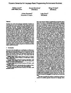
open Decl; ℓ := h; close Decl Let us consider one further example of a policy relating to dynamic change of an information flow lattice. Consider Figure 1 which depicts three information-flow lattices.

Figure 1. Example Dynamic Policy In the leftmost lattice Alice is the top element. While Alice is “boss” all information may flow to her. If she is demoted, however, then the information flow lattice changes to the central figure. From there either Bob or Alice can be promoted to be the boss. Let us consider how to encode this intended scenario with flow locks. A semantics for this policy is then provided by the flow locks semantics presented in the remainder of the paper. To represent this dynamic flow policy with flow locks we begin, not surprisingly, by assuming three actors: Alice, Bob, and Joe. To model the transitions between policies we use two locks: promoteA and promoteB. The events of promotion and demotion are modelled by the respective opening and closing of these locks. When promoteA is open then Alice is boss. Closing promoteA (respectively, promoteB) corresponds to demoting Alice (resp. Bob). To complete the picture we need to describe the corresponding policies for the data to be associated with Alice, Bob, and Joe. Joe is the simplest case, and his data has policy {Joe; Alice; Bob} – i.e. it is readable by everyone at all times. Alice’s data has policy {Alice; promoteB ⇒ Bob} and Bob has the symmetric policy {promoteA ⇒ Alice; Bob}. For Bob this means that his data is readable by Alice only when Alice has been promoted. Note that if both locks are open then we have a situation not modelled in the figure: Alice and Bob become equivalent from an information flow perspective. If we want to rule this out we cannot do so using the policy on data. We must enforce this via an invariant property of the locks themselves.

A Knowledge-based Approach One of the fundamental difficulties in the bisimulation-style definition is that it builds on a comparison between two runs of a system. While this is fairly intuitive for standard noninterference, in the presence of policy changes such as the opening or closing of locks (in our work) or declassification (in other work) it can be hard to see how the semantic definition really relates to what we can say about an attacker. One recent alternative to defining the meaning of declassification is to use a more explicit attacker model whereby one reasons about what an attacker learns about the initial inputs to a system as computation progresses [AS07]. The formulation we use here will be closest to [AHSS08]. The basic idea builds on a notion of noninterference described by [DEG06] and can be explained when considering the simple case of noninterference between an initial memory state, which is considered secret, and public outputs. The

Problems with the Flow Lock Security In our previous work we introduced a definition of what it means for a program to be secure with respect to a given assignment 3

value ⊥ to denote the least restrictive policy, for variables that all actors can see at all times. The opposite is the policy ⊤, which is simply the empty set of clauses, meaning no actor could ever see the data of a variable marked with that policy. To join two policies means combining their respective clauses. We define

model assumes that the attacker knows the program itself P . Now suppose that the attacker has observed some (possibly empty) trace of public outputs t. In such a case the attacker can, at best, deduce that the possible initial state is one of the following: K1 = {N | Running P on N can yield trace t }

p1 ⊔ p2 ≡ {Σ1 ∪ Σ2 ⇒ α|Σ1 ⇒ α ∈ p1 , Σ2 ⇒ α ∈ p2 }

Now suppose that after observing t the attacker observes the further output u. Then the attacker knowledge is

It should be intuitively clear that the join of two policies is at least as restrictive as each of the two operands, i.e. p ⊑ p ⊔ p′ for all p, p′ . In contrast, forming the union of two policies, i.e. the meet, corresponding to ⊓, makes the result less restrictive, so we have p ⊓ p′ ⊑ p for all p, p′ . Both ⊓ and ⊔ are clearly commutative and associative. We also need the concept of a policy specialized (normalized) to a particular lock state, denoted p(Σ), meaning the policy that remains if we remove from all guards the locks which are present in Σ. So for example, if p is {Paid ⇒ customer }, then p({Paid }) = {customer}. Formally, p(Σ) = {(∆ \ Σ) ⇒ α | ∆ ⇒ α ∈ p}.

K2 = {N | Running P on N can yield trace t followed by u } We will call K1 and K2 knowledge sets, and order knowledge sets by K ⊑ K ′ ⇐⇒ K ′ ⊆ K. Note that in the above K1 ⊑ K2 : the attackers knowledge increases as the computation proceeds. However, for the program to be considered noninterfering, in all such cases we must have K1 = K2 , since we require the knowledge to not increase at all throughout the program execution. This style of definition is the key to our new flow lock semantics. The core idea will be to determine what part of the knowledge must remain constant on observing the output u by viewing the trace from the perspective of the lock-state in effect at that time.

Operational Semantics To keep our presentation reasonably concrete we will consider imperative computation modelled by a standard small-step operational semantics defined over configurations of the form hΣ, c, M i where c (c′ , d etc.) is a command, M is a memory (store) – a finite mapping from variables to values, and Σ is the lock state – the set of locks that are currently open. We assume that each channel and variable x, y, . . . is assigned a fixed policy, where pol(x) denotes the policy of x. ℓ Transitions in the semantics are labelled hΣ, c, M i → h∆, d, N i where ℓ is either a distinguished silent action τ , or an observable action of the form x(v), where x is a channel and v is the value observed on that channel. We let w, w′ etc range over observable actions, and w ~ a vector of such. We assume the existence of commands which change the lock state. The open and close commands used in the concrete earlier work are sufficient, although other lock-state changing commands are possible. We do, however, assume that whenever the lock state changes then there is no output ℓ or memory change, i.e. if hΣ, c, M i → h∆, d, N i Σ 6= ∆ then we must have M = N and ℓ = τ . Given the labelled transition system we define some auxiliary notions.

3. Flow Lock Security In this section we motivate our flow sensitive definition of flow-lock security. The definition is phrased in terms of a labelled transition system where labels represent observable events. We assume an imperative computation model involving commands and stores (memories), but the definition is otherwise not specific to a particular programming language. 3.1 Preliminaries We begin by recalling the precise language of policies and introduce the base assumptions about the operational semantics of the language. Policies In general a policy p is a set of clauses, where each clause of the form Σ ⇒ α states the circumstances (Σ) under which actor α may view the data governed by this policy. Σ is a set of locks which we name the guard of the clause, and interpret it as a conjunction. Thus for the guard to be satisfied, all the locks σ ∈ Σ must be open. In concrete examples we will often simplify the notation, so that for example we will write (as we did in the introduction) {vendor ; Paid ⇒ customer } instead of

D EFINITION 3.1 (Visibility).

{∅ ⇒ vendor ; {Paid } ⇒ customer } .

• We say that x may be visible to α if Σ ⇒ α ∈ pol(x) for

A policy p is less restrictive than a policy q, written p ⊑ q, if for every clause Σ ⇒ α in q there is a clause Σ′ ⇒ α in p where Σ′ ⊆ Σ. For example, {vendor ; customer } is less restrictive than {vendor ; Paid ⇒ customer } which in turn is less restrictive than {vendor }. We use the distinguished

• We say that x is visible to α at ∆ if Σ ⇒ α ∈ pol(x) for

some Σ; otherwise we say that it is never visible. some Σ ⊆ ∆; otherwise we say that it is not visible at ∆. We extend these definitions to outputs x(v) in the same way, and we say that the silent output τ is never visible.

4

We define attacker visibility as a natural extension of actor visibility, by saying that x is visible to A = (α, ∆) iff x is visible to α at ∆. For each attacker we then define the A-observable transiw tion hΣ, c, M i →A h∆, d, N i by absorbing transitions which are not visible to attacker A.

3.2 Motivating the security definition To motivate our definition we will first look at some properties that we expect it to have. First we consider the case of simple declassification from the introduction. Consider the program ℓ := declassify (h); ℓ := h, which would be encoded as as

D EFINITION 3.3 (A-observable transitions). We can define w the transition relation →A as the least relation satisfying the following rules:

open Decl ; ℓ := h; close Decl ; ℓ := h The intended meaning of closing a lock is not that an actor should forget all they learned while the lock was open. Thus we expect this program to be considered secure, since the value of h is already known at the point of the second assignment. In other words, as we argued in section 2, we expect our definition to be flow sensitive, as opposed to our previous, bisimulation-based definition. Practically this means that our semantic definition cannot be a purely local stepwise definition, but requires us to inspect all knowledge gained by an attacker up to a certain assignment. Then we must validate that assignment in the context of the attacker having that knowledge. Another feature to note is that our flow locks system allows fine-grained flows, in which a secret may be leaked in a series of unrelated steps. The following policy and program exhibits this: x : {{Day, Night } ⇒ α}

y : {Night ⇒ α}

w

hΣ, c, M i → h∆, d, N i

w is visible to A

w

hΣ, c, M i →A h∆, d, N i ℓ

hΣ, c, M i → hΣ′ , c′ , M ′ i ℓ is not visible to A w hΣ′ , c′ , M ′ i →A h∆, d, N i w

hΣ, c, M i →A h∆, d, N i We now define some useful compound A-transitions. Firstly define hΣ, c, M i=⇒A h∆, d, N i if there is a sequence of zero or more transitions from hΣ, c, M i to h∆, d, N i with labels not visible to A. Now we define the multi-step A-observable w ~ transitions =⇒A for some sequence of output labels w ~ by ε equating =⇒A with =⇒A (where ε denotes the empty vector), and by inductively defining

z : {α}

w ~

w

hΣ, c, M i =⇒A hΣ′ , c′ , M ′ i →A h∆, d, N i

open Day; y := x ; close Day; open Night ; z := y

ww ~

hΣ, c, M i =⇒A h∆, d, N i

Here (and in subsequent examples) we assume each assignment generates an observable action – i.e. each variable is viewed as an output channel. Here the secret contained in x is leaked into z via y. But at the point where the assignment to z is made, the lockstate in effect does not allow a direct flow from x to z since Day is closed. In addition, at the point where the assignment to y is made, y is not visible at the current lockstate. To verify that this program is allowed, we need to validate the flows at each ”level” that the secret flows to, where a level corresponds to a certain set of locks guarding a location from a given actor. We note that these levels correspond to the points in the lattice Actors × P(Locks). This leads us to our formal attacker model:

w ~

We use the notation hΣ, c, M i=⇒A as a shorthand for w ~ ∃∆, d, N. hΣ, c, M i =⇒A h∆, d, N i, i.e. when we don’t care what the resulting configuration is. To reason about attacker knowledge we need to be able to focus on the parts of a memory which are visible to a given attacker. D EFINITION 3.4 (A-low memory, A-equivalence). Memory L is A-low for some attacker A if dom(L) = {x | x is visible to A}. We say that two memories M and N are A-equivalent, written M ∼A N if their A-low projections are identical – i.e. they agree on all variables that A can see.

D EFINITION 3.2 (Attacker). An attacker A is a pair of an actor α and a set of locks ∆, formally

We will adopt the convention that M and N will range over total memories (i.e. their domain will be the set of all variables). With this we can formalize the notion of attacker knowledge as follows:

A = (α, ∆) ∈ Actors × P(Locks) We refer to the lockstate component of an attacker as his capability, and assume that A can observe locations guarded from α only by locks in ∆. Intuitively we may think of an attacker as an actor who may open the locks ∆ at some point in the future, leading to a future-sensitive model3 that enables us to build secure commands by sequential composition from secure commands (see Section 4).

D EFINITION 3.5 (Attacker knowledge). The knowledge gained by an attacker A = (α, ∆) from observing a sequence of outputs w ~ of a program c starting with a A-low memory L written kA (w, ~ c, L), is defined to be the set of all possible starting memories that could have lead to that observation:

3 Future sensitivity is the one component of the original bisimulation-based definition that is retained in this new semantics.

w ~

kA (w, ~ c, L) = {M |M ∼A L, hΣ, c, M i=⇒A }

5

D EFINITION 3.9. (Termination Insensitive Flow Lock Security) A program c is said to be termination-insensitive Σ-flow lock secure, written T IF LS(Σ, c) iff for all attackers A = (α, ∆), all A-low memories L, and any two runs (ww, ~ Ω) and (ww ~ ′ , Ω′ ) in Run A (Σ, c, L) such that Ω ⊆ ∆ we have that kA (ww, ~ c, L) = kA (ww ~ ′ , c, L)

3.3 Flow Lock Security With this attacker model in hand, we can now formalise our security requirement. Intuitively, for a program to be flow lock secure we must consider the perspective of each possible attacker A, and how his knowledge of the initial memory evolves as he observes successive outputs. The requirement for each output thus observed is that knowledge of the initial memory only increases if the attacker’s inherent capabilities are weaker than the program lockstate in effect at the time of the output. The intuition here is that an attacker whose capability includes the program lock state in effect should already be able to see the locations used when computing the value that is output. Thus no knowledge should be gained by such an attacker. To formalize this intuition we first, for convenience, introduce the notion of a run. A run is just an output trace together with the lockstate in effect at the time of the last output in the sequence.

In this variant we allow some knowledge to be gained by the last step of the output, but no more than simply learning that there is an observable output. See [AHSS08] for more details. Note that by symmetry we compare the knowledge sets under both Ω and Ω′ .

4. Basic Properties of Flow Lock Security In this section we look at some basic properties of the definition of flow lock security. We inspect the basic properties of the definition via the principles of declassification as stated by Sabelfeld and Sands [SS05], since flow locks are intended to model various forms of declassification (or more generally reclassification).

D EFINITION 3.6 (Runs). The set of all runs of a command c starting with lock state Σ and with a starting memory whose A-low projection is L, are defined

Conservativity The conservativity principle states that in the absence of any declassification the security condition should revert to noninterference. As noted in [BS06a], we can model standard information-flow lattices by policies which contain sets of unguarded actors, so that for example in the two-point lattice Low ≤ High we would define two actors low and high, and then Low data would be modelled by the policy {∅ ⇒ low ; ∅ ⇒ high}, whereas High would correspond to {∅ ⇒ high}. In the presence of such unguarded policies it is straightforward to see that the notion of flow lock security reduces to the knowledge-based definition of noninterference from [AHSS08].

Run A (Σ, c, L) = {(ww, ~ ∆) | M ∼A L, w ~

w

hΣ, c, M i =⇒A hΣ′ , c′ , M ′ i →A h∆, d, N i} We can now define our security requirement in terms of runs as follows: D EFINITION 3.7 (Σ Flow Lock Security). A program c is said to be Σ-flow lock secure, written F LS(Σ, c), iff for all attackers A = (α, ∆), all A-low memories L, and all runs (ww, ~ Ω) ∈ Run A (Σ, c, L) such that Ω ⊆ ∆ we have kA (ww, ~ c, L) = kA (w, ~ c, L)

Monotonicity of release This principle states that adding more declassification to a “secure” program should never render it insecure. In the setting of flow locks, “adding more declassification” is naturally interpreted as opening more locks. A secure program which is modified to open more locks (but is otherwise unchanged) will still be secure since it is straightforward to see that the more locks are open in the lockstate at any given point in a trace, the weaker the flow lock security requirement at that point. Formally we can state the principle of monotonicity as follows:

This definition directly captures the intuition that we started out with. An attacker whose capabilities includes the current lockstate in effect at the time of the output should learn nothing new when observing that output. Attackers who do not fulfill this criterion have no constraint on what they may learn at this step. But note that this cannot lead to unchecked flows because we quantify over all attackers including, in particular, those with sufficient capabilities. At the top level we can define security for a self-contained program, i.e. one that doesn’t assume any locks are open before it starts:

P ROPOSITION 4.1 (Monotonicity of flow lock security). If F LS(Σ, c) and Σ′ ⊇ Σ then F LS(Σ′ , c).

D EFINITION 3.8 (Top-level Flow Lock Security). A program c is said to be flow lock secure, written F LS(c), iff the program is ∅-flow lock secure, i.e. F LS(∅, c).

The proof can be found in the appendix. Semantic consistency This states that the notion of security should be preserved by any semantics-preserving transformations to a program, and this is true for the semantics we define. One such example is dead code elimination. As mentioned in the introduction, lack of flow sensitivity makes

The above definitions are termination sensitive, since they require that no knowledge is gained by the simple observation that there is an output at all. Following [AHSS08] we can define a termination insensitive version: 6

security definitions sensitive to dead code. Here the definition of flow lock security can never be sensitive to dead code since it only quantifies over possible traces of a system – and these, by definition, are insensitive to dead code. It is worth noting that semantic consistency is relative to a particular semantics; in the concrete example that we consider in the next section we assume a semantics in which the effect of assignments are directly observable (to an appropriate attacker), something which does not hold for the usual operational semantics. This is referred to as a semantic anomaly [SS05], and is common to many security definitions which are phrased in terms of sequences of assignments.

The second minor obstacle to secure sequential composition is the lock state component. For this let us introduce Hoare-like triples {Σ}c{Σ′ }, which state that if any computation of c begins with at least locks Σ open, on termination at least locks Σ′ will be open.

Non-occlusion The non-occlusion principle is the most vague. It tries to capture the requirement that one declassification operation should not be able to mask an arbitrary amount of future insecure information flow. In our system we can argue for non-occlusion as follows. In our definition each assignment is considered in isolation, and the presumed knowledge gained from observing an assignment is exact. Therefore any further knowledge gained by observing any future assignment must still be subject to the same constraints (modulo the knowledge gained by the earlier assignment) with respect to the lock state and policies in force at that time. Adding declassifications therefore cannot mask future unintended flows.

In this section we will illustrate our definition of flow lock security to a specific language and type system, and prove that the type system guarantees flow lock security as given by the definition in the previous section. For the sake of brevity we treat just a simple while-language, but in principle we can apply the same approach to the higher-order language and type system in the style of that studied in [BS06a].

P ROPOSITION 4.2. The following proof rule is sound, assuming the concrete semantics uses visible termination: F LS(Σ, c1 )

{Σ}c1 {Σ′ } F LS(Σ′ , c2 ) F LS(Σ, c1 ; c2 )

5. Applicability: A Sound Type System

5.1 Language

hn, M i ⇓ n

hx, M i ⇓ M [x]

he1 , M i ⇓ v1 he2 , M i ⇓ v2 he1 ⊕ e2 , M i ⇓ v1 ⊕ v2

Hookup Properties for Sequential Composition In addition to the basic principles, it is useful to study composition principles (sometimes called hook-up properties [McC87]): when can we build secure programs from secure components. Here we briefly consider the most basic composition principle corresponding to sequential composition. Let us suppose that we have a sequential composition operator (either directly or encodable) with the usual semantics (see the next section for example). The termination sensitive condition has a technical problem that prevents it from composing sequentially: a program which ends in a silent loop is indistinguishable from one which terminates. This difference is revealed by composing the program with one which performs output. Termination insensitive flow lock security would consider the above composition secure, but still suffers from a problem, though for a different class of programs. A program that either silently terminates or produces one last output before termination is considered secure, since the silent termination is for all purposes equivalent to a silent loop. Composing such a program with one that performs an output again reveals the difference, and causes the previous output to be considered insecure. To obtain secure composition, the concrete semantics used may thus not have silent termination, i.e. all programs must produce a distinguished visible output if and only if they terminate. We say that such programs have visible termination. Our security definition from the previous section is agnostic as to whether visible termination is used or not.

τ

hΣ, open σ, M i → hΣ ∪{σ}, skip, M i τ

hΣ, close σ, M i → hΣ \{σ}, skip, M i he, M i ⇓ v x(v)

hΣ, x := e, M i → hΣ, skip, M [x 7→ v]i he, M i ⇓ v

v ∈ {true, false} τ

hΣ, if e then ctrue else cfalse , M i → hΣ, cv , M i τ

hΣ, while (e) c, M i → hΣ, if e then c; while (e) c else skip, M i ℓ

hΣ, c1 , M i → hΣ′ , c′1 , M ′ i ℓ

hΣ, c1 ; c2 , M i → hΣ′ , c′1 ; c2 , M ′ i τ

hΣ, skip; c2 , M i → hΣ, c2 , M i Figure 2. Operational Semantics The simple while language presented in Figure 2 will serve as the basis of our presentation. The only two nonstandard features are statements open σ and close σ for manipulating the program’s lock state. σ here ranges over single locks. The notion of observable action is defined (as 7

discussed in the previous section) as the action of assigning to a variable.

sures that no indirect flows leak information about a ”secret” conditional expression to ”public” locations. Similarly for the test r ⊑ w in the while rule. For the if rule, to compute a safe approximation to the locks that will be open it suffices to take the intersection of the resulting lock states of the branches. The while rule needs to use a fix point for the resulting lock state since one iteration of the loop may close locks that would then not be open in subsequent iterations. We note that there is a natural subtyping in the lock state component of this type system. Formally

5.2 Type System

⊢n:⊥

⊢ x : pol(x)

Σ ⊢ open σ ; ⊤, Σ ∪ {σ} Σ ⊢ skip ; ⊤, Σ

⊢ e1 : r1 ⊢ e2 : r2 ⊢ e1 ⊕ e2 : r1 ⊔ r2 Σ ⊢ close σ ; ⊤, Σ \ {σ}

⊢ e : r r(Σ) ⊑ pol(x) Σ ⊢ x := e ; pol(x), Σ

Σ ⊢ c ; w, Σ′ ∧ ∆ ⊇ Σ =⇒ ∆ ⊢ c ; w, ∆′ ∧ ∆′ ⊇ Σ′

⊢ e : r Σ ⊢ ci ; wi , Σi r ⊑ w1 ⊓ w2 Σ ⊢ if e then c1 else c2 ; w1 ⊓ w2 , Σ1 ∩ Σ2

This is easily proved by looking at all the uses of the lock states in the rules, and in particular noting that Σ is covariant in r(Σ) ⊑ pol(x) in the rule for assignment. Further, we can formalize our claim that the resulting lock state in the type system is a safe approximation of running the command as follows:

⊢ e : r Σ ∩ Σ′ ⊢ c ; w, Σ′ r ⊑ w Σ ⊢ while (e) c ; w, Σ′ ∩ Σ Σ ⊢ c1 ; w1 , Σ1 Σ1 ⊢ c2 ; w2 , Σ2 Σ ⊢ c1 ; c2 ; w1 ⊓ w2 , Σ2 Σ ⊢ c ; w, Σ′ Σ⊢c

P ROPOSITION 5.1 (Lockstate Safety). Σ ⊢ c ; w, Σ′ implies {Σ}c{Σ′ }.

(Top level judgement)

The proof of this is a straightforward induction over the typing derivations. We of course also want to prove soundness with respect to progress and preservation. We have that

Figure 3. Flow Lock Type System The type system we use can be found in figure 3. To simplify the presentation we use only int as base type for expressions, and commands have no base type, so we can restrict ourselves to only the flow locks aspects of the system. However, for convenience we use the boolean values false and true as shorthands for the value 0, and any value v 6= 0, respectively. For expressions we have judgements of the form ⊢ e : p where the policy p, called the read effect, is the join of the policies on all variables whose contents are used to produce its result. For commands the main judgements have the form Σ ⊢ c ; p, Σ′ . Here Σ is an assumption about what locks will be open before execution of c. The policy p is the so called write effect of a command, which is the union of the policies on all variables whose contents might be changed when executing the command. This plays a similar role to the “PC” level in many information flow type systems. The final component Σ′ is a safe approximation (i.e. an underestimation) of the locks that will be open after execution of c. Since the rules typically mention a number of different policies, we use r and w to range over read effect and write effect policies respectively, to simplify the presentation. Looking more closely at some of the rules, we note that, unsurprisingly, open and close are the only commands directly affecting the lock state. In the rule for assignments, the check r(Σ) ⊑ pol(x) ensures that the assignment is valid under the current lock state Σ, thereby ruling out leaks from direct flows. In the rule for if, the check r ⊑ w1 ⊓ w2 en-

P ROPOSITION 5.2 (Progress). If Σ ⊢ c ; w, ∆ and c 6= ℓ skip then hΣ, c, M i → hΣ′ , c′ , M ′ i. P ROPOSITION 5.3 (Preservation). If Σ ⊢ c ; w, ∆ and ℓ hΣ, c, M i → hΣ′ , c′ , M ′ i then Σ′ ⊢ c′ ; w′ , ∆′ for some ′ w ⊒ w and ∆′ ⊇ ∆. Proof of Progress is a straightforward case on the syntax of commands. Proof of Preservation is much more involved and can be found in the appendix. Finally we can state the main proposition of this section, which is that the type system implies flow lock security. The type system is formulated in a termination insensitive way, in particular we allow low assignments after high loops, so that is the formulation we will prove. T HEOREM 5.1 (Well typed programs are flow lock secure). If Σ ⊢ c then T IF LS(Σ, c). The proof is given in the appendix.

6. Example Encodings Many declassification ideas can now be encoded using flow locks – see [BS06b] for some examples. By such an encoding we now obtain a weaker flow-sensitive semantics for the corresponding declassification mechanism. 6.1 Delimited Non-Disclosure As a simple example let us take a more recent declassification mechanism, delimited non-disclosure [BCR08]. In its 8

simplest form we have variables of either High or Low security levels, and a local block-structured declassification command declassify h in c which allows a local weakening of the policy so that h is treated as low for the computation of command c. This is a variable-centric variant of Almeida Matos and Boudol’s nondisclosure construct [AB05]. To encode this idea using flow locks we need to use one lock Decl h per high variable h. Then we assign the policy pol(ℓ) = {high, low } for each low variable ℓ, and pol(h) = {high, Decl h ⇒ low } for each high variable h. The encoding of declassify h in c is then the obvious

hM, ei ⇓ n pol(x) 6= Low hM, x := ei → hM [x 7→ v], skipi hM, ei ⇓ n

pol(x) = Low

x(v)

hM, x := ei → hM [x 7→ v], skipi hM, ei ⇓ n r:x(v)

hM, x := declassify(e)i → hM [x 7→ v], skipi Figure 4. Operational semantics for Gradual Release

open Decl h ; c; close Decl h

release events denoted by r : x(v). Assignments to variables marked with High do not yield any outputs at all. The set of all possible low event sequences of a program is defined as follows:

For this encoding we need to assume that there are no nested declassifications over the same variable. This is not a real restriction since the inner declassification would be redundant in that case. The semantics of delimited non-disclosure is bisimulationbased with memory resetting, so suffers from flow insensitivity (see the example in Section 2). We conjecture that our encoding gives a strictly weaker semantics, but that encoded programs typable in our simple type system are also typable in the system given in [BCR08]. This is because our type system is too simple to take advantage of flow sensitivity.

D EFINITION 6.1 (Low event sequences). The set of all possible low event sequences that program c may generate starting from a low memory L is u ~

GRRun(c, L) = {~u | M =Low L, hM, ci =⇒hM ′ , c′ i} where =Low is equivalence on the low part of the memory. For a program to satisfy Gradual Release, it needs to fulfill the following property4:

6.2 Gradual Release

D EFINITION 6.2 (Gradual Release). A command c satisfies Gradual Release, written GR(c), if for all low projections of memories L, and all pairs of sequences ~uu, ~uu′ ∈ GRRun(c, L), we have

A more interesting example is provided by the Gradual Release property from [AS07]. This is interesting because the style of definition used there was the inspiration for our approach. Surprisingly we are able to show that, when specialised to the case of simple declassification, our definition coincides exactly with gradual release. We will begin by presenting their core operational semantics, as well as the Gradual Release security requirement for programs. We will then present a simple encoding of their language using flow locks, and show that for the class of flow locks programs conforming to the encoding, the two operational semantics and security requirements are equivalent. We will also show that their type system is equivalent to the type system given for the example language in Section 5, for that same class of programs. The language used in [AS07] is a simple while language similar to the one presented in section 5. It uses a simple two-level lattice L = {Low, High} with Low ⊑ High and High 6⊑ Low. As expected data may flow freely from locations marked with Low to locations marked with High, but not the other way around. The special declassify command allows a program to leak data from High to Low. The relevant parts of the operational semantics for this language can be found in Figure 4. There should be no surprises apart from the outputs arising from assignments and declassifications. These are labelled differently – normal assignments to variables marked with Low cause outputs of the form x(v) whereas declassifications output so called

k(c, L, ~uu) = k(c, L, ~uu′ ) Flow Locks Encoding The language displayed here is as noted already very similar to that shown in Section 5 and the encoding is straightforward as previously described. We define an encoding function b· over commands, and policies etc. First we need to represent the security levels High and Low. As before we introduce two actors: low is only allowed to see public (Low) data, while high is allowed to see any data. We also introduce a lock Decl to handle declassification. We can then encode the two levels as d = {high; Decl ⇒ low } and Low d = {high; low }. We High d d d d have Low ⊑ High and High 6⊑ Low, as expected. We exc) in the tend the encoding to variables (b x) and memories (M obvious way, by encoding all policies involved. Secondly, we need to encode declassification. As previously the command x := declassify(e) 4 We take

the liberty of presenting the definitions from [AS07] in a style that more closely resembles those which we have used for our own definitions. Our presentation is not different in any substantial way.

9

is represented with the sequence of commands

For declassification the rule from Gradual Release is simply ⊢GR e : r ⊢GR x := declassify(e) ; pol(x)

open Decl ; x := e; close Decl And that is all we need.

i.e. no constraints on the respective security labels of e and x. For the encoded equivalent,

Equivalence Our main goal here is to show that our encoding of the Gradual Release primitives leads to a system that is equivalent to the original Gradual Release system presented in [AS07]. In particular, we want to show that a program will be deemed secure according to Gradual Release if and only if its encoding is deemed flow lock secure.

open Decl; x := e; close Decl we can simply construct the derivation and everything is trivially typeable, with the exception of the constraint r({Decl }) ⊑ pol(x) arising from the assignment in the middle. Since we know from the domain that r is either {high; low } or {high; Decl ⇒ low }, we have that r({Decl }) = d Since for all l, Low d ⊑ l, the constraint {high; low } = Low. d Low ⊑ pol(x) is always fulfilled, and we are done.

GR(c) ≡ T IF LS(∅, b c) To do this, we first note that on the flow locks side the only possible lockstates at any point in the program are P(Locks) = {∅, {Decl}}, and the only actors are Actors = {high, low }. Further we note that for all attackers A ∈ Actors × P(Locks), the only attacker that would not have perfect knowledge of the memory at all times is A = (low , ∅). We can then specialise the definition of flow lock security, to say that an encoded program c is termination insensitive flow lock secure iff for attacker b b and all pairs of A = (low , ∅), for all A-low memories L, b we have that runs (ww, ~ ∅), (ww ~ ′ , Ω) ∈ Run A (∅, b c, L)

Discussion What we hope to show with this encoding is that this could have been a feasible (not to say easy) way to prove properties about Gradual Release. The proofs here that Gradual Release is a specialisation of Flow Locks are much less involved than the proofs in the Gradual Release paper, even though those are quite simple to begin with. Gradual Release is a special case in that it is already flow sensitive, so we get an exact equivalence between the original semantics and the flow locks induced one. We could not get such a correspondence with a flow insensitive system. However, we argue that most other systems are not inherently flow insensitive, and that giving a flow sensitive semantics to them via a flow locks encoding is not only feasible, but also beneficial since it makes it easier to relate various semantics and enforcement mechanisms. Reasoning about flow locks is greatly simplified by the new form of semantics. But what we have not done in these examples is take advantage of the fact that the semantic condition is not only simpler but also more liberal: in fact the type system we have presented is very similar to that which we previously verified against a flow insensitive semantics. Flow sensitivity would be useful in cases where the type system also needs to track properties of values – for example if we wanted to extend the typings to additionally verify that openings of locks only occurred in specific states, or released specific parts of some data (c.f. [BNR08]). Any resettingstyle semantics would not be able to track such properties through a computation.

b = kA (ww b kA (ww, ~ b c, L) ~ ′, b c, L) Next we note that we have a simple correspondance between the definitions of runs. L EMMA 6.1 (Correspondence between runs). If (~uu) ∈ b for A = GRRun(c, L) then (ww, ~ Ω) ∈ Run A (∅, b c, L) (low , ∅), and further Ω = {Decl} iff u is a release event, otherwise Ω = ∅. The proof of this is a straighforward inspection of c. Applying lemma 6.1 to our specialized version of flow lock security above, we end up with exactly definition 6.2, which is what we wanted to prove. Type system equivalence We can also show that the type system presented in [AS07] is equivalent to the type system presented in Section 5. The typing judgements and rules for expressions in the gradual release system are identical to those in our type system. For commands, we have that ⊢GR c ; w ⇐⇒ ∅ ⊢ b c ; w, b ∅ This is trivial to show for all commands except for assignments and declassifications. For assignments the rule for the Gradual Release system states that ⊢GR e : r r ⊑ pol(x) ⊢GR x := e ; pol(x) and we have a direct correspondence with the type rule for assignments from Section 5, specialised to encoded commands: \ ⊢ e : rb rb ⊑ pol(x)

7. Related Work As mentioned previously, the knowledge based approach used in this paper is inspired by the Gradual Release work [AS07]. Similar uses of knowledge sets appear earlier – e.g. [DEG06] – and many of the classic noninterference definitions have a knowledge or “deducability” flavour. However [AS07] appears to be the first to use this style of definition to reason about the semantics of declassification. Gradual release has also been extended by [BNR08] in a rather orthogonal direction, by allowing declassifications to carry a

\ ∅ ∅ ⊢ x := e ; pol(x), 10

References

logical specification of what is declassified, and under what condition. The notion of flow (in)sensitivity comes from the static analysis world, where it is used to characterise program analyses, and is not used to describe the underlying semantic property. The flow insensitivity problem arising in the papers mentioned in the introduction [MS04, EP05, EP03, AB05, Dam06, MR07, BCR08, LM08] all come about through somewhat related bisimulation-like definitions. But flow insensitivity can arise, in varying degrees, in other styles of model too. For example, [SHTZ06] deals with a detailed model of information flow policy updating. The semantics is phrased in terms of the trace segments in between policy updates, and asserts noninterference for the programs at the beginning of each of these segments. This is a resetting approach since it reasserts noninterference at intermediate program points, and thus becomes flow insensitive. As another example, flow insensitivity also arises in the definition of qualified robust declassification from [MSZ04] which uses a “scrambling” semantics for endorsement (upgrading of integrity) which nondeterministically resets the value of a variable after its endorsement. Flow locks do not deal directly with the question of what information is released (e.g. the length of a cryptographic key or the first four digits of a credit card number), and that is one natural direction for further work. In general policy mechanisms that deal with what is released are more extensional and therefore less prone to problems of context sensitivity. However a knowledge-style semantics can be useful in that setting too: a recent approach to expressive policies by Banerjee et al [BNR08] uses a generalisation of gradual release which is able to express policies which describe what is released (relative to the current state) at specific release points in the code. The policies include regular program assertions and can thus also constrain the conditions of release5 .

[AB05]

A. Almeida Matos and G. Boudol. On declassification and the non-disclosure policy. In Proc. IEEE Computer Security Foundations Workshop, pages 226–240, June 2005.

[AHSS08] A. Askarov, S. Hunt, A. Sabelfeld, and D. Sands. Termination insensitive noninterference leaks more than just a bit. In Proc. European Symp. on Research in Computer Security, 2008.

Acknowledgements Thanks to the ProSec group at Chalmers and the anonymous referees for useful comments and suggestions. This work was supported by the Swedish research agencies SSF, Vinnova, VR and by the Information Society Technologies programme of the European Commission under the IST-2005-015905 MOBIUS project. 5

In [BNR08] it is claimed in passing (p351) that the flow locks approach “is subsumed by our approach.” It is somewhat unclear in what sense flow locks are subsumed, but presumably this refers to the fact that flow locks can be viewed as boolean shadow variables, and as such can be used to express a conditional release policy in their setting. It not obvious to us how [BNR08] subsumes flow lock policies in any general sense since their work (i) only deals with a two-level low-high lattice, so cannot directly model multilevel security, integrity, and their combination (ii) only deals with declassification, and not e.g. upgrading of data or revocation of a principal’s clearance level, (iii) only allows declassification at an atomic step, and (iv) only deals with a termination sensitive security condition.

11

[AS07]

A. Askarov and A. Sabelfeld. Gradual release: Unifying declassification, encryption and key release policies. In Proc. IEEE Symp. on Security and Privacy, pages 207–221, May 2007.

[BCR08]

Gilles Barthe, Salvador Cavadini, and Tamara Rezk. Tractable enforcement of declassification policies. In Proc. IEEE Computer Security Foundations Symposium, 2008.

[BNR08]

A. Banerjee, D. Naumann, and S. Rosenberg. Expressive declassification policies and modular static enforcement. IEEE Symposium on Security and Privacy, pages 339–353, 2008.

[BS06a]

N. Broberg and D. Sands. Flow locks: Towards a core calculus for dynamic flow policies. In Programming Languages and Systems. 15th European Symposium on Programming, ESOP 2006, volume 3924 of LNCS. Springer Verlag, 2006.

[BS06b]

N. Broberg and D. Sands. Flow locks: Towards a core calculus for dynamic flow policies. Technical report, Chalmers University of Technology and G¨oteborgs University, May 2006. Extended version of [BS06a].

[Dam06]

M. Dam. Decidability and proof systems for languagebased noninterference relations. In Proc. ACM Symp. on Principles of Programming Languages, 2006.

[DEG06]

C. Dima, C. Enea, and R. Gramatovici. Nondeterministic nointerference and deducible information flow. Technical Report 2006-01, University of Paris 12, LACL, 2006.

[EP03]

R. Echahed and F. Prost. Handling harmless interference. Technical Report 82, Laboratoire Leibniz, IMAG, June 2003.

[EP05]

R. Echahed and F. Prost. Security policy in a declarative style. In Proceedings of the 7th International Conference on Principles and Practice of Declarative Programming (PPDP ’05), Lisboa, Portugal, July 2005.

[GM82]

J. A. Goguen and J. Meseguer. Security policies and security models. In Proc. IEEE Symp. on Security and Privacy, pages 11–20, April 1982.

[LM08]

Alexander Lux and Heiko Mantel. Who can declassify? In Preproceedings of the Workshop on Formal Aspects in Security and Trust (FAST), 2008.

[McC87]

D. McCullough. Specifications for multi-level security and hook-up property. In Proc. IEEE Symp. on Security and Privacy, pages 161–166, April 1987.

[MR07]

We can then see that using Ω′ ⊇ Ω in the implication is less restrictive since, Ω′ ⊆ ∆ will hold for fewer attackers.

H. Mantel and A. Reinhard. Controlling the what and where of declassification in language-based security. In Proc. European Symp. on Programming, volume 4421 of LNCS, pages 141–156. Springer-Verlag, March 2007.

Proof of Proposition 5.3 We need to show that ℓ

[MS04]

[MSZ04]

Σ ⊢ c ; w, ∆ ∧ hΣ, c, M i → hΣ′ , c′ , M ′ i

H. Mantel and D. Sands. Controlled downgrading based on intransitive (non)interference. In Proc. Asian Symp. on Programming Languages and Systems, volume 3302 of LNCS, pages 129–145. SpringerVerlag, November 2004.

=⇒ Σ′ ⊢ c′ ; w′ , ∆′ ∧ w′ ⊒ w ∧ ∆′ ⊇ ∆ which we do by induction of the height of the typing derivation. Case c = x := e: We know

A. Myers, A. Sabelfeld, and S. Zdancewic. Enforcing robust declassification. In Proc. IEEE Computer Security Foundations Workshop, pages 172–186, June 2004.

⊢ e : r r(Σ) ⊑ pol(x) Σ ⊢ x := e ; pol(x), Σ

[SHTZ06] N. Swamy, M. Hicks, S. Tse, and S. Zdancewic. Managing policy updates in security-typed languages. Computer Security Foundations Workshop, IEEE, 2006. [SS00]

[SS05]

[TZ04]

[ZM07]

ℓ

and hΣ, x := e, M i → hΣ, skip, M ′ i and can show that Σ ⊢ skip ; ⊤, Σ where ⊤ ⊒ pol(x). Case c = open σ: We must have

A. Sabelfeld and D. Sands. Probabilistic noninterference for multi-threaded programs. In Proc. IEEE Computer Security Foundations Workshop, pages 200–214, July 2000.

Σ ⊢ open σ ; ⊤, Σ ∪ {σ} and

ℓ

hΣ, open σ, M i → hΣ ∪ {σ}, skip, M i

A. Sabelfeld and D. Sands. Dimensions and principles of declassification. In Proc. IEEE Computer Security Foundations Workshop, pages 255–269, June 2005.

and the conclusion follows trivially. Case c = close σ: Like the case for open σ. Case c = if e then c1 else c2 : We must have

Stephen Tse and Steve Zdancewic. Run-time principals in information-flow type systems. In In IEEE Symposium on Security and Privacy, pages 179–193, 2004.

⊢ e : r Σ ⊢ ci ; wi , Σi r ⊑ w1 ⊓ w2 Σ ⊢ if e then c1 else c2 ; w1 ⊓ w2 , Σ1 ∩ Σ2

L. Zheng and A. C. Myers. Dynamic security labels and static information flow control. International Journal of Information Security, 6, 2007.

and ℓ

hΣ, if e then c1 else c2 , M i → hΣ, ci , M i for some i ∈ {1, 2}, and we have that Σ ⊢ ci ; wi , Σi and wi ⊒ w1 ⊓ w2 and Σi ⊇ Σ1 ∩ Σ2 . Case c = while (e) c: We have that

Appendix This appendix is not included in the published proceedings version of the paper. It includes proofs of the main results from the paper.

⊢ e : r Σ ∩ Σ′ ⊢ c ; w, Σ′ r ⊑ w Σ ⊢ while (e) c ; w, Σ′

Proof of Proposition 4.1 We need to show that and

F LS(Σ, c) ∧ Σ ⊆ Σ′ =⇒ F LS(Σ′ , c)

hΣ, while (e) c, M i

Assume F LS(Σ, c). That means that for all attackers A = (α, ∆), and all A-low memories L, we have that if (ww, ~ Ω) ∈ Run A (Σ, c, L) then Ω ⊆ ∆ =⇒ kA (ww, ~ c, L) = kA (w, ~ c, L) We make the following observations for using Σ′ ⊇ Σ: Changing the lock state will not affect control flow of a program, which means there will be a direct one-to-one mapping between elements in the two traces, with the same last element of the output sequence. For each element (ww, ~ Ω′ ) ∈ Run A (Σ′ , c, L) with a corresponding (ww, ~ Ω) ∈ Run A (Σ, c, L), we will have that Ω′ ⊇ Ω. The larger lock state is because adding more locks at the start can never lead to fewer locks open at any subsequent point in the program.

ℓ

→ hΣ, if e then c; while (e) c else skip, M i We can then construct the following derivation: ⊢e:r Σ ⊢ skip ; ⊤, Σ Σ ⊢ c; while (e) c ; w, Σ′ r⊑w Σ ⊢ if e then c; while (e) c else skip ; w, Σ′ ∩ Σ To prove that the sequential composition can indeed be typed we continue with Σ ⊢ c ; w, Σ′′ Σ′′ ⊢ while (e) c ; w, Σ′ Σ ⊢ c; while (e) c ; w, Σ′ 12

The first premise in this deriviation holds because of subtyping for lock sets, together with the observation that Σ ⊇ Σ ∩ Σ′ . By the subtyping rule we then also know that Σ′′ ⊇ Σ′ . To show the second premise we observe that

The proof follows directly from the construction of Run A (Σ, c, M \A ). Note also that this extends naturally to the case where we take more than one step and/or produce more than one output along the way.

⊢ e : r Σ′′ ∩ Σ′ ⊢ c ; w, Σ′ r ⊑ w Σ′′ ⊢ while (e) c ; w, Σ′ ∩ Σ′′

L EMMA .2 (Context typing). If Σ ⊢ E[c] ; w, Σ′ , then Σ ⊢ c ; wc , Σ′′ with w ⊑ wc . Proof: Straighforward induction on the typing derivation for E[c].

and note that this is an equivalent statement since Σ′′ ∩ Σ′ = Σ′ due to Σ′′ ⊇ Σ′ . Remains to show that Σ′ ⊢ c ; w, Σ′ . Since Σ′ ⊇ Σ′ ∩Σ we can show by subtyping of the original premise that Σ′ ⊢ c ; w, Σ′′′ where Σ′′′ ⊇ Σ′ . To see that Σ′′′ = Σ′ we note that by the subtyping rule we have that

L EMMA .3 (Deterministic expression evaluation). If ⊢ e : r and r is visible to A and he, M i ⇓ v then ∀M ′ ∼A M we have that he, M ′ i ⇓ v Proof: By induction on the structure of e. Case e = n: We have hn, M i ⇓ n for all M so the conclusion always holds. Case e = x: We have that hx, M i ⇓ (M [x]), and since pol(x) is visible to A and M ′ ∼A M we know that M ′ [x] = M [x]. Case e = e1 ⊕ e2 : By the assumption and the type rule for operators we know that r1 ⊔ r2 is visible to A, which implies that ri is visible to A, i ∈ {1, 2}. We apply the induction hypothesis to the subterms, and combine that with ⊕ being deterministic, and we are done.

Σ′′′ \ Σ′ ⊆ Σ′ \ (Σ′ ∩ Σ) = Σ′ \ Σ and the only way to satisfy that inequation is if Σ′′′ \Σ′ = ∅, hence Σ′′′ ⊆ Σ′ and we are done. Case c = c1 ; c2 : We have two cases, either c1 = skip or c1 6= skip. In the former case the conclusion follows trivially from the typing derivation and semantic rule, so the interesting case is the latter. We then have that Σ ⊢ c1 ; w1 , Σ1 Σ1 ⊢ c2 ; w2 , Σ2 Σ ⊢ c1 ; c2 ; w1 ⊓ w2 , Σ2 and

L EMMA .4 (Silent evaluation). If Σ ⊢ c ; w, ∆ and w is not visible to A, then running c with any starting memory will not produce any A-visible output, and will not change the memory in any way visible to A. Formally, ∀M we have either hΣ, c, M i =⇒A hΣ′ , skip, M ′ i

ℓ

hΣ, c1 ; c2 , M i → hΣ′ , c′1 ; c2 , M ′ i where the induction hypothesis gives us that Σ′ ⊢ c′1 ; w1′ , Σ′1 ∧ w1′ ⊒ w1 ∧ Σ′1 ⊇ Σ1

with M ′ ∼A M , or hΣ, c, M i ⇑A

We then have by subtyping that Σ′1 ⊢ c2 ; w2 , Σ′2 where Σ′2 ⊇ Σ2 , and thus we have that

Proof: By induction on the height of the typing derivation of Σ ⊢ c. Case c = x := e: We have

Σ′ ⊢ c′1 ; c2 ; w1′ ⊓ w2 , Σ′2 ∧ w1′ ⊓2 ⊒1 ⊓2 ∧ Σ′2 ⊇ Σ2

⊢ e : r r(Σ) ⊑ pol(x) Σ ⊢ x := e ; pol(x), Σ

and we are done. D EFINITION .1 (Bounded iteration). We define a bound on iteration of while-loops as follows:

Since pol(x) is not visible to A, for the transition ℓ

hΣ, x := e, M i → hΣ, skip, M [x 7→ v]i

[while (e) c]0 = skip

where he, M i ⇓ v, l is not visible to A, and M [x 7→ v] ∼A M. Case c = if e then c1 else c2 : We have

[while (e) c]k = if e then c; [while (e) c]k−1 else skip L EMMA .1 (Consistent run). If (w, ~ ∆) ∈ Run A (Σ, c, M \A ) and

⊢ e : r Σ ⊢ ci ; wi , Σi r ⊑ w1 ⊓ w2 Σ ⊢ if e then c1 else c2 ; w1 ⊓ w2 , Σ1 ∩ Σ2

hΣ, c, M i =⇒A hΣ′ , c′ , M ′ i

Neither w1 nor w2 are visible to A, so we can take a transition step

then (w, ~ ∆) ∈ Run A (Σ′ , c′ , M ′ \A ) Also, if (www ~ ′ , ∆) ∈ Run A (Σ, c, M \A ) and w

′

′

τ

hΣ, if e then c1 else c2 , M i → hΣ, ci , M i

′

hΣ, c, M i →A hΣ , c , M i using either transition rule for conditionals. We apply the induction hypothesis to the resulting term and we are done.

then (ww ~ ′ , ∆) ∈ Run A (Σ′ , c′ , M ′ \A ) 13

Case c = while (e) c′ : We have

where neither l nor l′ are visible to A, and M [x 7→ v] ∼A N [x 7→ v ′ ]. We continue by applying the induction hypothesis to the resulting configurations. Case c = E[if e then c1 else c2 ]: We have

⊢ e : r Σ ∩ Σ′ ⊢ c′ ; w, Σ′ r ⊑ w Σ ⊢ while (e) c′ ; w, Σ′ ∩ Σ To prove this case we need a contradiction. Assume that running c will produce a first output visible to A on the kth iteration, i.e. after first performing k−1 silent iterations. This means that up to the point of the first output, running c will be equivalent to running a bounded iteration [while (e) c′ ]k such that:

⊢ e : r Σ ⊢ ci ; wi , Σi r ⊑ w1 ⊓ w2 Σ ⊢ if e then c1 else c2 ; w1 ⊓ w2 , Σ1 ∩ Σ2 and we identify two cases: i) r is visible to A. Then by the deterministic expression evaluation lemma we have he, M i ⇓ v =⇒ he, N i ⇓ v. We must have

hΣ, [while (e) c′ ]k , M i =⇒A h∆, c′ ; skip, M ′ i

τ

hΣ, E[if e then c1 else c2 ], M i → hΣ, E[ci ], M i

′

with M ∼A M . We must then have and

w

h∆, c′ ; skip, M ′ i =⇒A h∆′ , c′′ ; skip, M ′′ i

τ

hΣ, E[if e then c1 else c2 ], N i → hΣ, E[ci ], N i

since the output cannot have come from the skip. But by the induction hypothesis and the typing of c we know that running c cannot produce any output visible to A, and we have our contradiction. Case c = c1 ; c2 : We apply the induction hypothesis to both subterms and we are done. The remaining cases for c can never produce any output or change the memory so they are trivial.

for the same i ∈ {1, 2}. We continue by applying the induction hypothesis to the resulting configurations. ii) r is not visible to A, which means w1 ⊓ w2 is not visible to A. Then by the silent evaluation lemma, and the fact that we know the computations cannot silently diverge before producing the output we seek, we must have that hΣ, E[if e then c1 else c2 ], M i =⇒A hΣ′ , E[skip], M ′ i

L EMMA .5 (Deterministic output). ww ~ If Σ ⊢, M ∼A N , hΣ, c, M i =⇒A hΣ′ , c′ , M ′ i and ww ~ hΣ, c, N i =⇒A hΣ′′ , c′′ , N ′ i then c′ = c′′ and M ′ ∼A N ′ .

and hΣ, E[if e then c1 else c2 ], N i =⇒A hΣ′′ , E[skip], N ′ i

Proof: By induction on the length of the transition sequence producing ww ~ when running with memory M . Case c = E[x := e]: We have

where M ′ ∼A M ∼A N ∼A N ′ . Since the lockstate cannot interfere with the evaluation or output, we can continue by applying the induction hypothesis to the configurations hΣ′ , E[skip], M ′ i and hΣ′ , E[skip], N ′ i. All other cases are trivial since only one transition rule applies, and that transition does not change the memory or produce any output. We simply perform that transition and apply the induction hypothesis to the resulting configurations.

⊢ e : r r(Σ) ⊑ pol(x) Σ ⊢ x := e ; pol(x), Σ and we identify two cases: i) pol(x) is visible to A. We must then have x(v)

hΣ, E[x := e], M i → A hΣ, E[skip], M [x 7→ v]i

L EMMA .6 (Deterministic silent termination). If Σ ⊢ c and M ∼A N and

and x(v)

hΣ, E[x := e], N i → A hΣ, E[skip], N [x 7→ v]i

hΣ, c, M i =⇒A hΣ′ , skip, M ′ i

where we have M [x 7→ v] ∼A N [x 7→ v]. If this was the final output then we are done, and that forms our base case for the induction. Otherwise we apply the induction hypothesis to the resulting configurations. ii) pol(x) is not visible to A. We then get

then either hΣ, c, N i =⇒A hΣ′′ , skip, N ′ i or hΣ, c, N i ⇑A .

ℓ

Proof: By induction on the length of the transition sequence leading to termination when running with memory M . Case c = skip: This case is only interesting since it forms the base case for the induction. skip trivially converges to skip in 0 steps with no output.

hΣ, E[x := e], M i → hΣ, E[skip], M [x 7→ v]i and ℓ′

hΣ, E[x := e], N i → hΣ, E[skip], N [x 7→ v ′ ]i 14

We prove this by showing that we must have w = w′ , by induction on the length of the computation leading to ww. ~ We identify two cases: i) w ~ has length greater than 0. Then by the deterministic output lemma, and the fact that we know both computations will produce more output and so cannot diverge, we must have that for M ∼A N :

Case c = E[x := e]: Since we know the computation is silent we must have that pol(x) is not visible to A. We then have ℓ

hΣ, E[x := e], M i → hΣ, E[skip], M [x 7→ v]i and ℓ′

hΣ, E[x := e], N i → hΣ, E[skip], N [x 7→ v ′ ]i

w ~

hΣ, c, M i =⇒A hΣ′ , c′ , M ′ i

for some v, v ′ . We have that neither l nor l′ are visible to A, and M [x 7→ v] ∼A N [x 7→ v ′ ], and we can apply the induction hypothesis to the resulting configurations. Case c = E[if e then c1 else c2 ]: We have

and

w ~

hΣ, c, N i =⇒A hΣ′′ , c′ , N ′ i where M ′ ∼A N ′ . By the consistent run lemma, subject reduction and non-interference of lockstates we then know that Σ′ ⊢ c′ and (w, Ω), (w′ , Ω′′ ) ∈ Run A (Σ′ , c′ , L′ ), where L′ is the common A-low projection of M ′ and N ′ , and we can apply the induction hypothesis to get w = w′ . ii) w ~ has length 0. We then proceed to case on c. Case c = E[x := e]: We have

⊢ e : r Σ ⊢ ci ; wi , Σi r ⊑ w1 ⊓ w2 Σ ⊢ if e then c1 else c2 ; w1 ⊓ w2 , Σ1 ∩ Σ2 and we identify two cases: i) r is visible to A. Then by the deterministic expression evaluation lemma we have he, M i ⇓ v =⇒ he, N i ⇓ v. We must have

⊢ e : r r(Σ) ⊑ pol(x) Σ ⊢ x := e ; pol(x), Σ

τ

hΣ, E[if e then c1 else c2 ], M i → hΣ, E[ci ], M i

and we identify two cases: i) pol(x) is not visible to A. Then

and τ

hΣ, E[if e then c1 else c2 ], N i → hΣ, E[ci ], N i

ℓ

hΣ, E[x := e], M i → hΣ, E[skip], M [x 7→ v]i

for the same i ∈ {1, 2}. We continue by applying the induction hypothesis to the resulting configurations. ii) r is not visible to A, which means w1 ⊓w2 is not visible to A. Then by the silent evaluation lemma we must have that

and ℓ′

hΣ, E[x := e], N i → hΣ, E[skip], N [x 7→ v ′ ]i We have that neither l nor l′ are visible to A, and M [x 7→ v] ∼A N [x 7→ v ′ ], and by the consistent run lemma we must have (w, Ω), (w′ , Ω′ ) ∈ Run A (Σ, E[skip], L) where L is the common A-low projection of the resulting memories. We can apply the induction hypothesis to get w = w′ . ii) pol(x) is not visible to A. Then the next transition will generate the visible output, so we must have Ω = Ω′ = Σ. Then by r(Σ) ⊑ pol(x) and ∆ ⊇ Σ we know that r is visible to A. Then by the deterministic expression evaluation lemma we know he, M i ⇓ v =⇒ he, N i ⇓ v, so we must have

hΣ, E[if e then c1 else c2 ], M i =⇒A hΣ′ , E[skip], M ′ i and either hΣ, E[if e then c1 else c2 ], N i =⇒A hΣ′′ , E[skip], N ′ i where M ′ ∼A M ∼A N ∼A N ′ , or hΣ, E[if e then c1 else c2 ], N i ⇑A . In the latter case we are done, in the former we apply the induction hypothesis to the resulting configurations. All other cases are trivial since only one transition rule could apply, and that transition does not change the memory nor produce any output. We simply perform that transition and apply the induction hypothesis to the resulting configurations.

x(v)

hΣ, E[x := e], M i → A hΣ, E[skip], M [x 7→ v]i and x(v)

Proof of Theorem 5.1 , repeated here for convenience. What we want to prove is Σ ⊢ c =⇒ T IF LS(c), which expanded means

hΣ, E[x := e], N i → A hΣ, E[skip], N [x 7→ v]i We have w = w′ = x(v) and we are done. Case c = E[if e then c1 else c2 ]: We have

∀A = (α, ∆), L, (ww, ~ Ω), (ww ~ ′ , Ω′ ) ∈ Run A (Σ, c, L)

⊢ e : r Σ ⊢ ci ; wi , Σi r ⊑ w1 ⊓ w2 Σ ⊢ if e then c1 else c2 ; w1 ⊓ w2 , Σ1 ∩ Σ2

we have that ∆ ⊇ Ω =⇒ kA (c, L, ww) ~ = kA (c, L, ww ~ ′)

and we identify two cases: 15

i) r is not visible to A. Then by the silent evaluation lemma and r ⊑ w1 ⊓ w2 we know the subterms cannot produce A-visible output. We must have hΣ, E[if e then c1 else c2 ], M i =⇒A hΣ′ , E[skip], M ′ i and hΣ, E[if e then c1 else c2 ], N i =⇒A hΣ′′ , E[skip], N ′ i with M ′ ∼A M ∼A N ∼A N ′ . By the consistent run lemma we must also have (w, Ω), (w′ , Ω′′ ) ∈ Run A (Σ′ , E[skip], L) and we can apply the induction hypothesis to get w = w′ . ii) r is visible to A. Then by the deterministic expression evaluation lemma we know he, M i ⇓ v =⇒ he, N i ⇓ v and we must have τ

hΣ, E[if e then c1 else c2 ], M i → hΣ, E[ci ], M i and τ

hΣ, E[if e then c1 else c2 ], N i → hΣ, E[ci ], N i for some i ∈ {1, 2}. By the consistent run lemma we must have (w, Ω), (w′ , Ω′′ ) ∈ Run A (Σ, E[ci ], L) and we can apply the induction hypothesis to get w = w′ . All other cases are trivial since only one transition rule applies, and that transition does not change the memory or produce any output. We simply perform that transition, note that the consistent run lemma applies, and apply the induction hypothesis to the resulting configurations.

16