deselect Inherit Part (NOTE, this is only needed for Windows OS), in Part text edit box click LMB and enter PNT (replacing GEOM), select Explicit Coordinates.
Lab 9: FLUENT: Transient Natural Convection Between Concentric Cylinders Objective: The objective of this laboratory is to introduce how to use FLUENT to solve both transient and natural convection problems. The specific problem considered is natural convection in the annular space between two concentric cylinders at different temperatures. Concepts introduced in this lab will include modeling options for transient flows, data storage, animations, and using the Boussinesq approximation for natural convection. Laboratory: For this problem we will model transient, two-dimensional flow of air due to natural convection in the annular space between two concentric cylinders as shown in Figure 1. The cylinders are assumed to be very long in the z-direction (into the paper), thus the flow can be modeled as twodimensional. Initially, the air in the gap is at uniform temperature T0 = 290 K. At time t = 0, the temperature of the inner surface is set to Ti = 310 K while the outer surface is kept at To = 290 K. As the air near the inner cylinder is heated its density decreases inducing an upwards flow. Due to continuity the cold air near the walls must go downwards and a circulating flow develops in the annular space.
y air filled space initially at T0 = 290 K
To = 290 K Ti = 310 K
x g Di = 0.020 m Do = 0.100 m
Figure 1. Schematic diagram of the natural convection flow in the annular space between long, horizontal, concentric cylinders.
In order to determine if the flow is laminar or turbulent within the annular space we must calculate the Rayleigh number typically defined for this geometry as
g β (Ti − To ) L3c RaLc = = 1.96 × 10 4 να
€
Lc =
[
]
2 ln(ro ri )
(
ri −3 /5 + ro −3 /5
(1)
43
)
5 /3
= 0.0220 m
(2)
where g is the gravitational acceleration, β is the thermal expansion coefficient, ν is the kinematic viscosity, and α is the thermal diffusivity at the average temperature in the annular space defined as Tm = (€Ti + To ) 2 . For this Rayleigh number the flow is well within the laminar region. The total heat transfer rate from one cylinder to the other at steady state has been studied experimentally by Raithby and Hollands [1] and a correlation for the heat transfer rate per unit length is given as a function of an effective thermal conductivity € keff ⎛ ⎞1 4 1 4 Pr = 0.386 ⎜ (3) ⎟ RaLc = 3.74 ⎝ 0.861+ Pr ⎠ k
qʹ′ = €
€
q 2 π keff (Ti − To ) = = 7.68 W/m L ln(ro ri )
(4)
where k is the molecular thermal conductivity. This correlation is good for 0.7 ≤ Pr ≤ 6000 and RaLc ≤ 10 7 . € Laboratory: € ICEM CFD To run ICEM CFD, click on the ICEM CFD icon on the desktop. In the Main Menu, from the Settings pull down menu select Product. In the DEZ verify under Product Setup that ANSYS Solvers - CFD Version is selected. If it is not, do so, click OK, exit the program, and then restart ICEM CFD. Step 1. Select Working Directory and Create New Project Main Menu - From File pull down menu, select Change Working Directory using LMB. In New Project directory dialog box create a new folder. Do not use a name with spaces, including all the directories in the path. Main Menu - From File pull down menu, select New Project using LMB. In New Project dialog box create a new project. Again, do not use a name with spaces. Step 2. Create Points for Geometry Function Tab - From Geometry select Create Point
2
using LMB.
DEZ - For Create Point enter the following: deselect Inherit Part (NOTE, this is only needed for Windows OS), in Part text edit box click LMB and enter PNT (replacing GEOM), select Explicit Coordinates using LMB, under Explicit Locations ensure Create 1 point is selected from pull down menu, in Y text edit box click LMB and enter 10 for point at (0, 10, 0), click Apply using LMB and verify the Message Done: points pnt.00, in Y text edit box click LMB and enter -10 for point at (0, -10, 0), click Apply using LMB and verify the Message Done: points pnt.01, in Y text edit box click LMB and enter 50 for point at (0, 50, 0), click Apply using LMB and verify the Message Done: points pnt.02, in Y text edit box click LMB and enter -50 for point at (0, -50, 0), click Apply using LMB and verify the Message Done: points pnt.03, in Y text edit box click LMB and enter 0, in X text edit box click LMB and enter 10 for point at (10, 0, 0), click Apply using LMB and verify the Message Done: points pnt.04, in X text edit box click LMB and enter 50 for point at (50, 0, 0), click Apply using LMB and verify the Message Done: points pnt.05, click Dismiss using LMB. Utilities - Select Fit Window
using LMB to verify that six points have been created.
Geometry DCT - Expand Geometry and Parts menus by using LMB to change + to - for each.
Under Model\Geometry use RMB to click on Points and select Show Point Names using LMB. Verify that six points have been created.
From Points Step 3. Create Curves for Geometry The From Points allows you to select createCreate/Modify a Bspline curve Curve by interpolating Function Taboption - From Geometry usingthrough LMB. n number of points. From Points DEZ - For Create/Modify Curve enter the following: Click on the iconInherit and select location on the screen to create points that define a curve. ensure Partany is NOT selected,
in Part text edit box click LMB and enter WALL_INNER (replacing PNT), Arc Arc from select 3 Points
using LMB, under Method ensure From 3 Points is selected from pull down menu, select Select LMB, The Arc option allows youlocation(s) to create anusing arc from three points. select pnt.00, pnt.04, and pnt.01 using LMB to create inner arc, verify the Message Done: curves crv.00, From 3 Points Part text box three click LMB Creates ainBspline arc edit through points.and enter WALL_OUTER, select pnt.02, pnt.05, and pnt.03 using LMB to create outer arc, Center and 2verify Points the Message Done: curves crv.01, •
Radius If enabled, the radius will be setusing as the specified value. If disabled, the radius will be set at the distance select From Points LMB, in Part click LMB and enter SYMMETRY, between thetext firstedit twobox points selected.
•
select pnt.00 and pnt.02 using LMB and then click MMB to create upper boundary,
Keepverify Center Start/End theorMessage Done: curves crv.02,
select pnt.01 and pnt.03 using LMB and then click MMB to create lower boundary,
The Keep optionDone: will take the first point selected as the center, the second point as the first verifyCenter the Message curves crv.03, arc beginning, and calculate the arc end from the vector defined by the first point and third point. click DISMISS using LMB. The radius used will be determined by the Radius parameter. The Keep Start/End option will use the first and second points selected as the arc ends and calculate the center using the Radius parameter if specified, or else the average distance between the first 3 and second points, and the first and third points. The plane will be defined by the three selected points. •
Points
Figure: 2D Blocking Transform Blocks
Step 4. Create Blocking
Edit Edge Pre-Mesh Params Pre-Mesh Quality Pre-Mesh Smooth Block Checks Delete Block
Create Function Tab - From Blocking select CreateBlock Block
Associate
using LMB.
DEZ - For Create Block enter theFigure: following: Create Block Options in Part text edit box click LMB and enter FLUID, Figure: Blocking Associations Options under Initialize Blocks Type select 2D Planar from pull down menu, and click Apply and Dismiss using LMB.
Associate Split Function Tab - From Blocking select SplitBlock Block
using LMB. Figure: Blocking Associations Options DEZ - For Split Block enter the following: under Split Method select Prescribed point from pull down menu, select Select edge(s) using LMB, select right edge of block using LMB, select pnt.05 at ( 0, 50, 0) using LMB to options create horizontal split, The following are available forand creating blocks: click Dismiss using LMB. The Initialize Block options are available for blocking associations. following From Vertices/Faces
Associate Vertex (in contrast to curves and points for the NOTE: The block is made up of edges and Face vertices Extrude to Curve geometry). For the block, boundary Associate edges areEdge colored black and the interior edge is light blue.
2D to 3D Blocks Associate Edge to Surface 3D to 2D The following are splitting blocks:use Associate to Surface DCT - Expand Blocking menu by using LMBFace to options change + toavailable - . Underfor Model\Blocking Split Block LMB to check the box for Vertices and then use RMB to click on Vertices and select Numbers from Geometry TheDisassociate following options are available for blocking associations. Ogrid Block using LMB. Verify that six vertices are now numbered. You may want to make the point names Update Associations Associate Vertex invisible to clearly see the numbers for the vertices. Extend Split Reset Associations Associate Edge to Curve Split Face Snap Project Associate Edge Vertices to Surface Split Vertices Group/Ungroup Curves Associate Function Tab - From Blocking select Associate using LMB. Associate Face to Surface Split Free Face ANSYS ICEM CFD 13.0 - © SAS IP, Inc. All rights reserved. - Contains proprietary and confide Auto Associate Disassociate from Geometry formation of ANSYS, Inc. and its subsidiaries and affiliates. Imprint Free Face DEZ - For Blocking AssociationsUpdate enter the following:Associations Options Figure: Blocking Associations Reset Associations Associate Vertex under Edit Associations select Associate Vertex using LMB, Snap Project Vertices select Select vert(s) usingGroup/Ungroup the LMB, Curves select Vertex number 33 and then pnt.04 atVertex (10, 0,option 0) using the LMB, The Associate allows you to associate vertices and project the v Auto Associate select Vertex number 13 and then pnt.00 at (0, 10, 0) using the LMB, curves, and surfaces. Select theCFD vertex to project onto. and confid ANSYS ICEM 13.0 - © and SAS IP, the Inc. Allentity rights reserved. - Containsit proprietary 336 formation of ANSYS, Inc. and its subsidiaries and affiliates. select Vertex number 11 and then pnt.01 at (0, -10, 0) using the LMB,
select Vertex number 21 and then pnt.02 at (0, 50, 0) using the LMB, Vertex select Vertex number 19 Associate and then pnt.03 at (0, -50, using the LMB, Associate Edge to0)Curve select Vertex number 34 and then pnt.05 at (50, 0, 0) using the LMB,
The Associate Vertex option allows you to associate vertices and project the ver The Associate Edge to Curve option allows you to associate the edges of bloc the end of the edges are also associated to the same curve unless they were p The following are available associations. curve or point.options Edge segments can for be blocking individually associated after using edge Associate Vertex associated with multiple curves, but allusing the curves Edge totoCurve under Edit Associations Associate select Associate Edge Curve LMB, will be grouped into a single Associate Edge to Curve select Select edge(s) using the LMB, Edge to Surface Associate select Edges number 13-33 11-33 using and then click MMB, Theand Associate Edge to Curve option allows you to associate the edges of blocks NoteFace Associate to LMB Surface select Curve crv.00 usingthe LMB and then click MMB, end of the edges are also associated to the same curve unless they were pre Disassociate from Geometry select Edges number 21-34 and 19-34 using LMB and then MMB, in the curve or point. Edge segments can click be associated using edge sp Associating edges to curves alsoindividually results creationafter of line elements al Update Associations select Curve crv.01 usingassociated LMB and then click MMB, with multiple curves, but all the curves will be grouped into a single c 2D planar blocking, it is essential that all the perimeter edges be associate ResetLMB Associations select Edge number 13-21 using and then click MMB, because many solvers use the perimeter line elements as boundaries. Snapand Project select Curve crv.02 using LMB thenVertices click MMB, Group/Ungroup Curves Note Auto Associate Project vertices Associating edges to curves also results in be theprojected creation of elements alon If enabled, the vertices will automatically to line the corresponding 4 2D planar blocking, it is essential that all the perimeter edges be associated Project to surface intersection Associate Vertex because many solvers use the perimeter line elements as boundaries. If enabled, the surface-surface intersection will be captured correctly. This is where the intersection curve may not match with the intersection of the su
curves, surfaces. Select thethey vertex the entity to aproject NOTE: All vertex colors will turn from and black to red indicating areand associated with point. it onto.
Selected Block Mesh Factor of Two sets Figure: the shape of only the Scaled selectedby edge.
In dimension sets the shape automatically for all connected edges. Select the source edge f the Source index or vertex, and the Target index or vertex.
select Edge number 11-19 using LMB and then click MMB, select Curve crv.03 using LMB and then click MMB, and click Dismiss using LMB.
Unlink Edge
NOTE: All outer block edge colors will turn to green indicating they are associated with a curve.
The Unlink Edge option allows you to unset the shapes of edges linked by the L
Step 5. Mesh Blocks and Surface
Pre-Mesh Params Function Tab - From Blocking select Pre-Mesh Params
using LMB.
DEZ - For Pre-Mesh Params enter the following: Figure: Pre-Mesh Parameters Options
Edge under Meshing Parameters select EdgeParams Params using LMB, scroll down and select Copy Parameters using LMB, TheParallel Edge Params allows youpull to modify the mesh parameters in a under Copy Method ensure To All Edgesoption is selected from down menu, scroll up and select Select Edges(s) using LMB, laws and the node spacing along any particular edge. Ea various bunching select Edge number 13-21 using that LMB, determine the spacing of the mesh along the edge: number of nodes under Mesh law select Geometric 1 from pull down menu, at the beginning/end of the edge, the expansion of the mesh from the be under Spacing enter 0.4 for spacing for first nodes from surface, interior, and the maximum element length along the edge. under Nodes enter 41,
The Edge Params icon brings up a window with all the mesh parameters
The LMB, following options are available for Pre-Mesh parameters: select Select Edges(s) using the mesh parameters for that edge will be displayed. All parameter values Update Sizes select Edge number 13-33 using LMB, Edge the menu, Edge Length, which are pre-defined. Scale Sizes under Mesh law select Uniform from ID pulland down under Nodes enter 50, Edge Params Match Edges
select Select Edges(s) using LMB, Refinement select Edge number 11-33 using LMB, under Mesh law select Uniform from pull down menu, ANSYS ICEM CFD 13.0 - © SAS IP, Inc. All rights reserved. - Contains proprietary an under Nodes enter 50, Update Sizes formation of ANSYS, Inc. and its subsidiaries and affiliates. click Dismiss using LMB.
The Update Sizes option allows you to update sizes in the pre-mesh. The followin DCT - Under Model\Blocking use LMB to check the box for Pre-Mesh. In Mesh Dialog Box select Yes to compute mesh. for updating sizes in the pre-mesh:
Update All computes the edge node spacing based on constraint equations with the def Step 6. Save Files and Export Mesh law. You can adjust the number of nodes on each edge based on the Global S Size and by default each edge will follow the BiGeometric geometry law.
NOTE: You should produce a structured mesh with nodes concentrated near the inner wall.
Main Menu - From File pull down menu, select Blocking -> Save Unstructured Mesh using LMB. Use the Save Mesh as Dialog Box to save the unstructured mesh.
ANSYS ICEM CFD 13.0 - © SAS IP, Inc. All rights reserved. - Contains proprietary and confidenti
374menu, select Save Project usingformation Main Menu - From File pull down LMB.of ANSYS, Inc. and its subsidiaries and affiliates.
Function Tab - From Output select Output To Fluent V6 using LMB. In Family boundary conditions dialog box: expand SYMMETRY menu by using LMB to change + to -, click Create new to open the Selection dialog box, under Boundary Conditions select symmetry using the LMB, click Okay using LMB to close the Selection dialog box, expand WALL_INNER menu by using LMB to change + to -, click Create new to open the Selection dialog box,
5
under Boundary Conditions select wall using the LMB, click Okay using LMB to close the Selection dialog box, expand WALL_OUTER menu by using LMB to change + to -, click Create new to open the Selection dialog box, under Boundary Conditions select wall using the LMB, click Okay using LMB to close the Selection dialog box, click Accept using LMB. In Open dialog box click Open to select unstructured mesh with current project name. In Fluent V6 dialog box enter the following: in Grid dimension select 2D using LMB, in Scaling ensure No is selected, in Write binary file ensure No is selected, in Ignore couplings ensure No is selected, in Boco file retain the default file name, in Output file change the file from fluent to a new name for your mesh, and click Done using LMB.
6
FLUENT Step 1. Read In Mesh Import your mesh created using ICEM CFD into FLUENT. Check to make sure the mesh imported correctly and that you scale it correctly from mm to m. Step 2. Problem Setup for Initial Simulation In the Navigation Pane under Problem Setup use the following steps to setup your simulation: General • Solver o Type: Pressure-Based o Time: Transient o Velocity Formulation: Absolute o 2D Space: Planar • Gravity: ON • Gravitational Acceleration o x-direction: 0 m/s2 o y-direction: -9.81 m/s2 Models (remaining models off) • Energy: On • Viscous: Laminar Materials, Fluid, air (change the properties for air to those at 300 K) • Density: Boussinesq (use pull down menu), 1.1614 kg/m3 • Specific Heat: 1,007 J/kg•K • Thermal Conductivity: 0.0263W/m•K • Viscosity: 1.846e-05 kg/m•s • Thermal Expansion Coefficient: 0.00333 1/K (where β = 1/Tm for an ideal gas) Cell Zone Conditions • Zone: fluid o Type: fluid o Material Name: air • Operating Conditions o Operating pressure: 101,325 Pa o Gravity: ON (gravitational acceleration set using Problem Setup: General) o Boussinesq Parameters • Operating Temperature: 290 K (use cold temperature for enclosure) • Specified Operating Density: ON • Operating Density: 1.1614 kg/m3 Boundary Conditions • Zone: symmetry o Type: symmetry • Zone: wall-inner o Type: wall
7
•
o Edit: Momentum tab • Wall Motion: Stationary Wall • Shear Condition: No Slip o Edit: Thermal tab • Thermal Conditions: Temperature • Temperature: 310 K, constant Zone: wall-outer o Type: wall o Edit: Momentum tab • Wall Motion: Stationary Wall • Shear Condition: No Slip o Edit: Thermal tab • Thermal Conditions: Temperature • Temperature: 290 K, constant
Reference Values • Compute from: wall-inner • Reference Zone: air-flow Step 3: Solution Setup for Simulation In the Navigation Pane under Solution use the following steps to setup your solution methods, controls, monitors, and initialization: Solution Methods • Pressure-Velocity Coupling o Scheme: PISO (more efficient for transient) • Spatial Discretization o Gradient: Least Squares Cell Based o Pressure: Body-Force Weighted (good for natural convection flows) o Momentum: Second Order Upwind o Energy: Second Order Upwind • Transient Formulation: Second Order Implicit • Non-Iterative Time Advancement: ON (again, more efficient option) Solution Controls • Non-Iterative Solver Relaxation Factors o Pressure: 1 o Momentum: 1 o Energy: 0.9 (required for natural convection to get convergence) Monitors • Residuals - Print, Plot o Options • Print to Console: ON • Plot: OFF o Equations, Residual, Monitor: ON (all 4 equations) • Surface Monitors (click Create to open Surface Monitor Dialog box) o Name: heat_flux_mon (change from default of surf-mon-1) o Options
8
• Print to Console: OFF • Plot: ON, Window: 1 • Write: OFF • x Axis: Flow Time • Get Data Every: 1 Time Step (use pull down menu) o Report Type: Integral o Field Variable: Wall Fluxes, Total Surface Heat Flux o Surfaces: wall-inner NOTE: We are using surface monitors to plot total heat flux from inner cylinder versus time. We will use a second window to make an animation of the solution. Before we set that up below from the Menu Bar select View -> Graphics Window Layout and then an option that allows you to see two panes in the Graphics Window. Solution Initialization (which is actually setting the initial condition) • Reference Frame: Relative to Cell Zone • Initial Values o Gauge Pressure: 0 Pa o x Velocity: 0 m/s o y Velocity: 0 m/s o Temperature: 290 K Calculation Activities • Autosave Every: 10 Time Steps (use Edit button to change file name and location) • Solution Animations (click Create/Edit to open Solution Animation Dialog Box) o Animation Sequences: 1 o Name: vectors o Every: 10 Time Step o Define (to open Animation Sequence Dialog Box) Storage Type: Metafile Window: 2 (hit Set button) Display Type: Vectors (should open Vectors Dialog Box or hit Edit button) • Vectors of: Velocity • Color by: Temperature, Static Temperature • Options o Global Range: ON o Auto Range: OFF o Clip to Range: OFF o Auto Scale: ON o Draw Mesh: OFF • Scale: 4, Skip: 2 • Min: 290 K, Max: 310 K Click Display button in the Vectors Dialog Box to make a plot of the velocity vector field in window 2. You should see the outline of your domain, but no vectors because your initial velocity field is zero. Hit the Close button to close the Vectors Dialog Box and hit the OK button to close the Animation Sequence Dialog Box. In the Solution Animation Dialog Box verify that the vectors sequence is now checked as Active and hit the OK button to close the Dialog Box. You can now pan or zoom for a different view of the velocity vector field in window 2 if desired for your animation, but the default view should be fine.
9
Step 4. Run Calculation Navigation Pane - Under Solution select Run Calculation. Task Page - Under Time Step Size enter 0.005 s, under Number of Time Steps enter 200 and click Calculate. Next, select the Calculate button in the Task Page. Note that at each time step the solution must iterate until convergence, but this only takes usually 2 iterations for PISO/NITA. The heat transfer from the inner cylinder versus flow time should appear in window 1. Its value starts out high and then decreases to below 5 W after about 1 second. Every 10 time steps the converged velocity vector field colored by temperature should appear in window 2. Notice that a hot plume rises from the inner cylinder and then re-circulates downwards near the outer wall. Step 5. View Solution Animation Navigation Pane - Under Results select Graphics and Animations. Task Page - Under Animations select Solution Animation Playback and select Set Up to open Playback Dialog Box. Use the controls to view the animation. If you want to make an MPEG movie of the animation change WRITE/Record Format to MPEG and click WRITE button. Step 6. View Solution at Each Time Step To display the velocity vector data at any previous time step, from the Main Menu select File\Read\Data and select a data file to read in one that was automatically saved during the run. In the Task Page under Graphics and Animations select Vectors and select Set Up to open the Vectors Dialog Box. Under Vectors of select Velocity and under Color by select Temperature and Static Temperature from the pull-down menus. Select Display to see the plot in the Graphics Window. Step 7. Continue Simulation If desired you can solve for velocity and temperature at additional time steps with the same or different time step. To continue make sure that you have open the data file you wish to proceed from. The new plots will be appended to your existing animation by default. If you run the simulation until it reaches steady state the heat flux converges to 7.36 W (which is doubled to include both halves of the annulus). This compares well with the 7.68 W predicted by Equation (4) with an approximately 4% difference (reasonable for an experimental correlation). Assignment There is no written assignment due for this lab so that you can work on the final project (see my webpage at www.calpoly.edu/~kshollen and follow the ME 544 link to a link for the final project assignment and an example validation paper). There is also a link to “FLUENT Summary” under the General Course Notes section that lists instructions for running a typical simulation.
10