Fluid Flow Animation Jakov Fustin, Zeljka Mihajlovic University of Zagreb, Faculty of Electrical Engineering and Computing, Unska 3, 10000 Zagreb Department of Electronics, Microelectronics, Computer and Intelligent Systems, E-mail:
[email protected],
[email protected]
phone: (+385) 1 6129 521; fax: (+385) 1 6129 653
Abstract – In this paper we briefly outline theoretical fundamentals of fluid dynamics as well as present a model for computer based simulation. Of special interest are target driven smoke simulations which don't require expert knowledge in order to achieve desired results. One of such methods was presented and implemented in two dimensions using programming language C++. The results obtained are presented alongside parameters that affect the progress of simulation. Keywords: fluid dynamics, target-driven animation
I. INTRODUCTION We are all witnessing the appearance of more and more special effects in movies and video games. They add to overall impression and make us talk about them for days. Sometimes, they are put up just to compensate for the lack of story and/or good acting, but that’s not the subject here. What matters to us is what happens behind the scene and how these effects are created. Of all special effects, the most challenging are natural phenomena, such as fluids in motion (e.g. smoke and water). A lot of work has been done to create realistic animations of fluids. The first models were operating with particles [1] and suffered from not being physically accurate. Navier-Stokes equations, which present a physical model for fluid flow, came into use later when Chen et al. [2] implemented them in two dimensions to animate water surface. Foster and Metaxas [3] went further to use the full Navier-Stokes equations in three dimensions and obtained many effects that were hard to key frame automatically. Their solver is explicit and becomes unstable for large time steps. Stam [4] introduced an unconditionally stable algorithm based on an implicit solver which lets users add smoke into the system and apply forces without fear of simulation blowing up. More recently, methods for controlling fluid flow have been developed. Treuille et al. [5] introduced a technique that causes a smoke simulation to optimally approximate a set of user specified key frames. While it produces good results, it is also computationally demanding and thus slow. Fattal and Lischinski [6] presented a method that does not guarantee the key frames to be optimally approximated but also demands less processor power. The rest of this paper gives a brief introduction to fluid dynamics (Section 2) and presents Stam’s model (Section 3) and later Fattal and Lischinski’s method (Section 4) for simulation of fluid flow on computer. In Section 5 we describe our implementation of target-driven smoke solver and finally, in Section 6, we present results obtained by it.
II. FLUID DYNAMICS Fluid mechanics is the branch of physics that studies fluids. It can be subdivided into fluid statics and fluid dynamics. The former concerns itself with fluids at rest and the latter studies fluids in motion. Since this paper talks about animating fluid flow, fluid dynamics will be of primary interest. 2.1 Euler and Navier-Stokes equations The state of any moving fluid in 3-D space is completely determined with five physical quantities: three components of velocity and two thermodynamic quantities such as density and pressure. All these quantities are functions of coordinates and time. u = u x (x, t ) i + u y (x, t ) j + uz (x, t ) k p = p(x, t ) r = r (x, t ) To find out the state of a fluid at some time t, we must compute all of the five quantities using physical laws known as conservation of mass, conservation of momentum and conservation of energy. After combining these three laws, we get Euler equations for incompressible inviscid fluid flow ¶u 1 = - ( u × Ñ ) u - Ñp + a ¶t r
(1)
¶r = - ( u ×Ñ ) r ¶t Ñ × u = 0.
(2)
Right hand side terms in (1) account for advection, hydrostatic pressure and external forces respectively, while (2) conserves the mass. To account for viscosity, additional considerations have to be made, the result of which are Navier-Stokes equations for incompressible homogeneous (¶r/¶t = 0) viscous fluid flow ¶u 1 m = - ( u × Ñ ) u - Ñp + Ñ 2 u + a ¶t r r Ñ × u = 0.
(3)
The new term on the right hand side of (3) is
m 2 Ñ u, r
where m represents dynamic viscosity.
III. COMPUTATIONAL MODEL Simulation of fluid flow on computer comes down to numerical integration of Euler (or, as in this paper, Navier-Stokes) equations. First, we must write them in a form that is suitable for computer implementation and then make discretizations along time and space axes. 3.1 Helmholtz-Hodge decomposition Using Helmholtz-Hodge decomposition on (2) and (3), we obtain a single equation for the velocity ¶u æ m ö = P ç - ( u × Ñ ) u + Ñ 2u + a ÷ , ¶t r è ø
(4)
where P represents an operator that projects a vector field onto its divergence free part (therefore, condition Ñ × u = 0 is implicit). This form will be used in computer implementation. 3.2 Space and time discretization The space is divided into equally sized parallelepipeds that are called cells. State variables can be positioned inside these cells in two ways, each of which has its advantages.
The first way is to define all quantities at the center of each cell (easier to implement, but susceptible to checkerboard instability). The other way is to define velocity variables at the centers of cell faces and leave only pressure and density at the center of each cell (avoids checkerboard instability). Since the space is no longer continuous, operator Ñ changes from Ñ = (¶/¶x, ¶/¶y, ¶/¶z) to Ñ = (Δ/Δx, Δ/Δy, Δ/Δz). Finally, (4) is written in the following form to account for time discretization u * -u æ m ö = P ç - ( u ×Ñ ) u + Ñ2 u + a ÷ , Dt r è ø
(5)
where u represents velocity at some time t, and u* represents velocity at t+Δt. 3.3 Moving substances Non-reactive substances moving through the fluid (e.g. a drop of ink in the water) are advected by it and satisfy the following equation ¶r = - (u × Ñ ) r + k r Ñ2 r - ar r + Sr , ¶t
(6)
where κr is diffusion constant, αr is dissipation rate and Sr represents external sources. Like (4), this equation too has to be discretized over time and space. 3.4 Solving Navier-Stokes equations Since the similarity of (4) and (6) is obvious, same methods can be used to find their solution. Stam describes this in detail in [4] so we'll skip it here.
IV. TARGET-DRIVEN SIMULATIONS
Fig. 1. All quantities defined at cell centers.
While the model described above provides the means for a user to affect the progress of a simulation (by modifying term a in (4) and term Sr in (6)), it is very hard to achieve desired results. This is due to nonlinearity of (4) and numerical dissipation. It would be nice if user only had to specify the desired state and the simulation evolved to it spontaneously. Such methods are crucial for animators because they let them create convincing special effects not seen before. 4.1 Modified Navier-Stokes equations This paper focuses on the method developed by Fattal and Lischinski [6]. They make a few modifications to (5): u * -u = P ( - ( u × Ñ ) u + v f F ( r , r *) - vd u ) , Dt
Fig. 2. A staggered grid.
(7)
where r = r ( x,t ) is density of the substance moving through the fluid and r * = r * ( x ) is the desired density. Term a is replaced by v f F ( r , r *) which is a driving force, i.e. it drives the substance to the desired state r* and:
F ( r , r *) = r '
Ñr '* . r '*
(8)
The term -vd u attenuates momentum. Equation (6) is modified as follows: ¶r = - ( u ×Ñ ) r + vg G ( r , r *) , ¶t
(9)
where vg G ( r , r *) is a smoke gathering term and G ( r , r *) = Ñ × ëé rr '* Ñ ( r - r *) ûù .
method here is MakeStep that computes state variables at a time t+Δt. A step consists of six smaller steps as shown below: void TDSmokeSolver::MakeStep ( ) { void applyDrivingForce ( ); void attenuateMomentum ( ); void advectMomentum ( ); void project ( ); void advectSmoke ( ); void gatherSmoke ( ); }
(10)
More information about r', r'*, F ( r , r *) and G ( r , r *) can be found in [6]. All of the three new terms are controlled by nonnegative parameters vf, vd and vg.
Before we describe every element of MakeStep method, a few things have to be said. We used a staggered grid, with variables positioned as shown in fig. 2. On this grid, discrete derivative and average operators are defined as follows:
4.2 Solving modified Navier-Stokes equations
Dx ( u )i , j =
Method of solution is similar to the one described in [4] and can be found in [6]. The main difference is in the approach to solve the advection term - (u × Ñ ) u . Stam uses the unconditionally stable semi-Lagrangian scheme, while Fattal and Lischinski use the second order hyperbolic solver based on Lax-Wendroff formula which is subject to a time step restriction.
V. IMPLEMENTATION We implemented the method described in previous chapter in C++ programming language. Some fragments from Stam's code were used, but for the most part, the program was written from the scratch. 5.1 Data structures and algorithms
Ay ( r )i , j +1/ 2 =
Since this is a 2-D solver, there are only four (instead of five) state variables: u, v, r and p. Simulation parameters are denoted by vf, vd, vg and sigma variables. The key
- ui -1/ 2, j )
Dx u ( i+3 / 2, j - 2ui+1/ 2, j + ui-1/ 2, j )
(r
( Dx )2
i , j +1
+ ri , j ) 2
.
Now we’ll show the pseudocode for the first step, which applies the driving force using (8). It is pretty much straightforward, so no explanations other than that already present in [6] are necessary. void { // // // //
TDSmokeSolver::applyDrivingForce ( ) Fu D_rts A_rt A_rts
-> -> -> ->
horizontal derivative average of average of
component of the force of ro tick star ro tick ro tick star
// horizontal component - u for ( every_cell u[i,j] ) { double Fu, D_rts, A_rt, A_rts;
class TDSmokeSolver { protected: // state variables std::vector u, v, r, p; // ro star, ro tick, ro tick star, ro gather std::vector rs, rt, rts, rg; // simulation parameters double vf, vd, vg, sigma;
public: // a big step void MakeStep ( ); };
i +1/ 2, j
Dxx ( u )i +1/ 2, j =
The base of the program is TDSmokeSolver class that solves (7) and discretized form of (9). An excerpt from the header file follows:
// six small steps that make one big step void applyDrivingForce ( ); void attenuateMomentum ( ); void advectMomentum ( ); void project ( ); void advectSmoke ( ); void gatherSmoke ( );
(u
D_rts = ( A_rt = ( A_rts = ( Fu = A_rt } }
rts[i,j] - rts[i-1,j] ) / delta_x; rt [i,j] + rt [i-1,j] ) / 2.; rts[i,j] + rts[i-1,j] ) / 2.; * D_rts / A_rts;
u[i,j] += dt * vf * Fu;
// the same goes here for vertical component
The second step attenuates the momentum through -vd u term and is the easiest to implement. void TDSmokeSolver::attenuateMomentum ( ) { // horizontal component - u for ( every_cell u[i,j] ) u[i,j] -= dt * vd * u[i,j];
}
// vertical component - v for ( every_cell v[i,j] ) v[i,j] -= dt * vd * v[i,j];
The advection term - ( u ×Ñ ) u is solved using second order hyperbolic solver. Details for implementing such solver can be found in Appendix A of [6]. Protected methods hyperbolicSolveU and hyberbolicSolveV contain our implementation of the solver for x and y axis respectively.
void TDSmokeSolver::gatherSmoke ( ) { // step one for ( every_cell rg[i,j] ) rg[i,j] = r[i,j] - rs[i,j]; // step two for ( every_cell rg[i,j] ) rg[i,j] += dt * hyperbolicSolveU(…) / delta_x + dt * hyperbolicSolveV(…) / delta_y;
void TDSmokeSolver::advectMomentum ( ) { // horizontal component - u for ( every_cell u[i,j] ) u[i,j] -= dt * hyperbolicSolveU(…) / delta_x;
}
// step three for ( every_cell rg[i,j] ) rg[i,j] *= r[i,j] * rts[i,j]; // step four for ( every_cell rg[i,j] ) rg[i,j] += dt * hyperbolicSolveU(…) / delta_x + dt * hyperbolicSolveV(…) / delta_y;
// vertical component - v for ( every_cell v[i,j] ) v[i,j] -= dt * hyperbolicSolveV(…) / delta_y;
The projection is done differently for inner and boundary cells because it depends on cell’s neighbors. While all inner cells have four neighbors, boundary cells have three or even only two neighbors. void TDSmokeSolver::project ( ) { // this term appears in all three cases below for ( every_cell div[i,j] ) div[i,j] = ( u[i+1,j] - u[i,j] + v[i,j+1] – v[i,j] ) * delta;
}
// step five for ( every_cell r[i,j] ) r[i,j] += vg * rg[i,j];
5.2 Graphical user interface Graphical user interface was created with MFC (Microsoft Foundation Classes). It is pretty simple and easy to use.
// compute pressure for ( int k=0; k