NavierâStokes equations for incompressible viscous fluid. ... in particular, the work starts from the need to describe currents in a complex environment including ...
ESAIM: PROCEEDINGS,
March 2012, Vol. 35, p. 263-268
F´ ed´ eration Denis Poisson (Orl´ eans-Tours) et E. Tr´ elat (UPMC), Editors
FLUID FLOW MODELING IN COMPLEX AREAS ∗, ∗∗
Jean–Marc Mounsamy, Jacques Laminie and Pascal Poullet 1 Abstract. We show first results of 3D simulation of sea currents in a realistic context. We use the full Navier–Stokes equations for incompressible viscous fluid. The problem is solved using a second order incremental projection method associated with the finite volume of the staggered (MAC) scheme for the spatial discretization. After validation on classical cases, it is used in a numerical simulation of the Pointe ` a Pitre harbour area. The use of the fictious domain method permits us to take into account the complexity of bathymetric data and allows us to work with regular meshes and thus preserves the efficiency essential for a 3D code.
R´ esum´ e. Dans cette ´etude, nous pr´esentons les premiers r´esultats de simulation d’un ´ecoulement d’un fluide incompressible visqueux dans un contexte environnemental r´eel. L’approche utilis´ee utilise une m´ethode de domaines fictifs pour une prise en compte d’un domaine physique tridimensionnel tr`es irr´egulier. Le sch´ema num´erique combine un sch´ema de projection incr´ementale et des volumes finis utilisant des volumes de contrˆ ole adapt´es ` a un maillage d´ecal´e. Les tests de validation sont men´es pour les cas tests de la cavit´e double entraˆın´ee ainsi que l’´ecoulement dans un canal avec un obstacle plac´e de mani`ere asymm´etrique.
Introduction The aim of the present work is a description of the dynamics of water–sea currents in a three–dimensional rigid lid environment; in particular, the work starts from the need to describe currents in a complex environment including the harbour of Pointe–` a–Pitre in the archipelago of Guadeloupe (FWI). Due to the complexity of the domain, environmentmal flows require often the use of the fully 3D Navier–Stokes equations (NSE) [DPB06]. That is what we deal with, in a first step. Subsequently, we will able to compare our results with other models (model using the hydrostatic hypothesis, Shallow–Water model). One of our long term goals is to provide a hydro–sedimentary model of this area to describe the morphological evolution process. As we know these models of sediment transport are derived mainly from the Exner law which is an hyperbolic PDE [HS03]. Here, we choose a finite volume discretization to avoid coupling problems that might occur between the two models. Moreover, new trends investigate to couple finite volume method with finite element method (FEM) to combine the advantages of the two approachs (specifically the use of finite elements is well appropriated to the treatment of boundary of general shape). For large 3D models, the FEM, even coupled with another method, leads to store matrices of huge size that is preferable to be avoided. In this context, we use uniform cells in finite volume and to take into account the irregularities of the domain with uniform parallelepipedic cells, This work has been supported by a partnership between the Port Autonome de Guadeloupe and Universit´ e des Antilles et de la Guyane ∗∗ Computational tests have been obtained by the server Orca of the Centre Commun de Calcul Intensif of the Universit´ e des Antilles et de la Guyane 1 Universit´ e des Antilles et de la Guyane, LAMIA, Campus de Fouillole, Pointe–` a–Pitre, Guadeloupe FWI c EDP Sciences, SMAI 2012
∗
Article published online by EDP Sciences and available at http://www.esaim-proc.org or http://dx.doi.org/10.1051/proc/201235025
264
ESAIM: PROCEEDINGS
approximations have been made using the fictitious domain techniques. Even though, this fictitious domain method has been introduced more than three decades age [Pes77], it is known to be reliable [ABF99], and relevant in our context. The domain of fluid of realistic shape is then complemented by another fictitious domain so that their addition composes a rectangular parallelepiped. The fictitious domain method that has been used involves adding a penalized velocity term in the momentum equation of the incompressible Navier– Stokes equations. Only the parts of our domain which are close to the boundary of our obstacle or inside our obstacle are penalized. One of the advantages of such a method is that it avoids body–fitted unstructured meshes and allows regular Cartesian meshes. The use of the staggered Marker And Cell (MAC) mesh provides us a stability property and prevents us from dealing with spurious pressure and velocity fields. A second order backward difference formula (BDF2) is used for the time approximation and a second–order Richardson extrapolation for the nonlinear term. The pressure and velocity terms are computed following a fractional step method (standard incremental projection) scheme providing us a scheme which is second order accurate in time for the velocity [FLPA09]. Our paper is organized as follows: first, we introduce the model that is considered in our solver. Second, we further explore the numerical approximation of this model including the penalization method, which allows to take into account obstacles. The last part is devoted to the initial numerical results which have been obtained using our solver.
1. Our CFD solver The primary goal for our work is solving the problem in a complex area which is given by a bathymetric survey. Hence, let us consider a general domain Ω (a regular bounded connected open set of IR3 ) that contains M regular solid bodies ΩiS of IR3 (1 ≤ i ≤ M ). The index ‘S’ stands for the solid bodies immersed in the i fluid, while the index ‘f ’ stands for the fluid domain. Thus, let ΩS be equals to ∪M i=1 ΩS . The obstacles are penalized by enforcing the velocity to be small in the domains that represent them. Thus, we are seeking u η , pη ), the velocity field and the pressure, which satisfy the following problem in two steps. Then, we compute (u the approximate velocity with (
u η + u η · ∇u u η + η1 1ΩS uη + ∇pη ∂t uη − ν∆u ∇ · uη
= F
in Ω × [0, T ]
= 0
in Ω × [0, T ]
(1)
augmented with the initial and boundary conditions: u η uη · n − p n ν∇u u η|t=0
= uD
on
ΓD × [0, T ]
=
on
ΓN × [0, T ]
in
Ω,
F /ΓN
= u0
(2)
where n represents the normal vector to the boundary ΓN . We denote by Ωf the domain of the incompressible viscous flow: Ωf = Ω \ ΩS , Γ = ∂Ω = ΓN ∪ ΓD , ΓN ∩ ΓD = ∅, with meas(ΓD ) 6= ∅. As in the physical case, the motion is obtained by forcing a non homogeneous Dirichlet boundary condition on ΓD , while ΓN constitutes the part of our boundary where an outflow boundary condition is imposed. To simulate the motion of the water in the real environment, we use the hydrodynamic survey provided by our partner, the Port Autonome de la Guadeloupe. Regarding to the bay survey chart, one obtains a domain of the fluid (Ωf ) with an irregular shape. Indeed, this bay includes areas with shallow depth where coastal and inshore navigation take place, two small islands and a deeper channel mainly used by merchant ships. Moreover the bay is bordered by mangrove areas in some places, small beaches elsewhere, and constructions included the harbour everywhere else. One finds at the south of the domain, the chanel entrance, and at the northern part,
265
ESAIM: PROCEEDINGS
a small strip of sea that is named la Rivi`ere Sal´ee, which splits the two main islands of Guadeloupe. One can easily recognize the importance of the study especially since this strip of sea links a nature reserve le Grand Cul de Sac Marin to the bay that we consider. The strategy that we apply, is to complete this domain with solid fictitious bodies to form a recyangular parallelepiped Ω. Thus, this approach enables us to combine fictitious domain method with finite volume discretization using uniform cells.
2. Discrete scheme 2.1. Time advancing scheme We use a classical projection method to solve our problem. Among the class of projection methods [GMS06], the standard incremental projection is chosen for its efficiency and accuracy. Indeed, this second order accurate method is decomposed into two steps. The first one consists of computing an approximate velocity by solving an elliptic problem: 1 (3˜ ˜ k+1 uk+1 − 4ukη + uηk−1 ) − ν∆˜ uk+1 + η1 1ΩS u η η η 2δt k k−1 k+1 +((2uη − uη ).∇)˜ uη + ∇pkη ˜ k+1 = uD , (ν∇˜ u uk+1 · n − pk n)| η|Γ
D
η
η
ΓN
= F(tk+1 ),
(3)
= 0,
and the second one is devoted to update the pressure while correcting the velocity (which corresponds to the projection onto the divergence–free functional space). The projection step can be described as follows : 3 (uk+1 − u ˜ k+1 ) + ∇(pk+1 − pk ) 2δt ∇ · uk+1 uk+1 · n pk+1
= = = =
0, 0, uk+1 ·n D k p
on on
ΓD , ΓN ,
(4)
where n still represents the normal vector to the boundary ΓD . By applying the divergence operator to the first equation of (4) and after substitution of the second equation, one obtains an elliptic problem for the pressure with Neumann boundary condition, which is quite easy to solve. Hence, the velocity is updated by the equation : ˜ k+1 − uk+1 = u
2δt ∇(pk+1 − pk ). 3
2.2. Spatial discretization Let Ω be our sufficiently regular domain in IR3 . Let τ = (Ki,j,k )i=1,..,N1 ; j=1,...,N2 ; k=1,...,N3 be an admissible mesh of Ω in the sense of assumption 3.2 of [EGH00] extended to 3D domain. As we use a staggered mesh, p u v w we need to consider 4 different meshes Ki,j,k , Ki,j,k , Ki,j,k , Ki,j,k , each of them associated with each velocity component and the pressure. Hence, the finite volume scheme comes from the problem (3) which has been ∗ integrated over each control volume Ki,j,k of the velocity component considered. Whenever possible, the volume R R integrals are computed via the Gauss theorem: K u ∆u dX = ∂K u ∇u . n dσ, with n being the normal to i,j,k i,j,k u u the boundary ∂Ki,j,k , outward to Ki,j,k . Thus, our control volumes being parallelepipeds, their boundary is a collection of 6 faces that cover them. Let Γi be one of the faces of an interior control volume K (such that Γi 6∈ ∂Ω). Let L be a control volume neighbour of K, such that Γi = K ∩ L. The flux through this face is
266
ESAIM: PROCEEDINGS
computed by a standard finite difference formula: Z Z UL − UK ∇u.ndσ ≈ ∇u . ndσ ≈ × meas(Γi ), dK/L Γi Γi where dK/L is the distance between the centers of the control volume K and L. One can easily shows that this flux approximation is conservative and consistant. ∗ In the case where one face (or more than one) of a control volume Ki,j,k is a part of the boundary of our domain Ω, the flux through this face is computed differently. One introduces outside of the domain a fictitious control volume of the same size as the other control volumes. The value of the solution in this control volume is fixed such that the boundary condition on this part of the domain is verified.
3. Numerical Results A computer program has been developed in object–oriented Fortran. In order to validate the code, two test problems have been solved. First, to check the Navier–Sokes solver with Dirichlet boundary conditions, we solved the double lid driven cavity problem in 3D. Second, we solved a channel flow in a rectangular parallelepiped without any obstacle to check the approximation of the outflow boundary condition. We then considered to introduce an obstacle by using the fictitious domain technique. Initial results for the realistic domain of the bay of Pointe–` a–Pitre are given, including few modifications of the bay survey.
3.1. Double lid driven cavity problem in 3D The initial velocity field and pressure are set to zero. As our scheme is a two–steps scheme, we compute the first iterate with the one–step Euler method. Only the second component of the velocity is nonzero at the top of the domain. The main structures of the flow are obtained. Indeed, the section cut located at the middle of the domain shows two large eddies and the small eddies at the corners of the bottom are emphasized (see first plot of figure 1). The 3D aspect of the flow is well demonstrated (see second plot of figure 1) .
Figure 1. Double lid driven cavity problem in 3D at T = 1.4 with 64 × 64 × 128 cells in the domain [0, 1]2 × [0, 2], the viscosity parameter ν = 10−3 (section cut at the middle of the domain).
ESAIM: PROCEEDINGS
267
3.2. Simulation of a channel flow around an obstacle We aim to show in this section the efficiency of the fictitious domain technique that is called L2 -penalization. Then, an obstacle is simulated by setting the value of the penalization parameter η equals to 10−4 . Setting a very small viscosity parameter ν = 10−4 requires certainly the finest mesh that we were able to use. As one can observe in figure 2, the flow is unsteady and has a coherent behaviour. The figure displays that the flow avoids the obstacle and many eddies are created in the domain. Moreover, there is no problem of stability of the flow downstream close to the boundary. Hence, the approximation of the outflow boundary condition is well done.
Figure 2. Channel flow at T = 0.5 with 128 × 128 × 32 cells in a parallelepipedic domain [0, 1] × [0, 3] × [0, 0.4] with an obstacle in a nonsymmetric location.
3.3. First numerical results of the real domain The mesh and data files for the fictitious domain method have been computed from the bathymetry survey given by Le Port Autonome de Guadeloupe. The shallow areas are missing. Therefore the coast is approximately defined as well as the mangrove swamp. Only the harbor entrance of the port and la Rivi`ere Sal´ee are modelized. Moreover, some connections are not available between the port and le Petit Cul Sac Marin (on the left part of the figure 3). On the left part of figure 3 we present one of our first numerical simulation results of sea currents for the Pointe–` a–Pitre harbour. An aerial picture of the port is shown on the right–hand side including the bathymetric data. The velocity field is displayed. It is clear that the main part of the flow follows the deeper area of the harbour. The outfall of la Rivi`ere Sal´ee is very narrow so that the output flow is quite strong.
268
ESAIM: PROCEEDINGS
These results are very encouraging. More computation are in progess simulating the tides and some improvement on the bathymetry data is also planned.
Figure 3. Environmental flow obtained in a domain Ω = [0, 3000] × [0, 5000] × [0, 17] with a mesh of 240 × 360 × 35 cells, the viscosity parameter ν = 10−4 , and η = 10−7 .
References [ABF99]
Ph. Angot, C.–H. Bruneau, and P. Fabrie. A penalization method to take into account obstacles in incompressible viscous flows. Numer. Math., 81:497–520, 1999. [DPB06] A. Deponti, V. Pennati, and L. De Biase. A fully 3d finite volume method for incompressible Navier–Stokes equations. Int. J. Numer. Meth. in Fluids, 52:617–638, 2006. [EGH00] R. Eymard, T. Gallou¨ et, and R. Herbin. The finite volume method, volume VII of Handbook of Numerical Analysis. 2000. [FLPA09] C. F´ evri` ere, J. Laminie, P. Poullet, and Ph. Angot. On the penalty–projection method for the Navier–Stokes equations with the MAC mesh. J. Comput. Appl. Math., 226(2):228–245, 2009. [GMS06] J.–L. Guermond, P. Minev, and J. Shen. An overview of projection methods for incompressible flows. Comput. Meth. Appl. Mech. Engng., 195:6011–6045, 2006. [HS03] J. Hudson and P.K. Sweby. Formulations for numerically approximating hyperbolic systems governing sediment transport. J. Scient. Comput., 19(1–3):225–252, 2003. [Pes77] C. Peskin. Numerical analysis of blood flow in the heart. J. Comput. Phys., 25:220–252, 1977.