FLUID LIMITS OF PURE JUMP MARKOV PROCESSES: A PRACTICAL GUIDE R. W. R. Darling National Security Agency P. O. Box 535, Annapolis Junction, MD 20701
[email protected] July 10, 2002
ABSTRACT: A rescaled Markov chain converges uniformly in probability to the solution of an ordinary differential equation, under carefully specified assumptions. The presentation is much simpler than those in the outside literature. The result may be used to build parsimonious models of large random or pseudo–random systems.
1. INTRODUCTION ‡ 1.1 Our Goal In many fields of research one seeks to give a parsimonious description of the behavior of a large system whose dynamics depend on the random interactions of many components (molecules, genes, consumers, …). Such a description may take of the form of the solution of an ordinary differential equation, derived as the deterministic limit of a suitably scaled Markov process, as some scale parameter N ö ¶. We are especially interested in applications to large random combinatorial structures, in order to extend results such as those presented in Bollobás (2001), Kolchin (1999), and Janson, ∆uczak and Rucinski (2000). The study of such limit theorems is a rich, and technically advanced, topic in probability: see the books of Ethier and Kurtz (1986) (esp. p. 456), and Jacod and Shiryaev (1987) (esp. p. 517). The work of Aldous, e.g. Aldous (1997), offers many examples of the application of modern probabilistic limit arguments to random combinatorial structures. Our goal here is to establish a fairly general fluid limit result, accessible to anyone familiar with basic Markov chains, Poisson processes, and martingales. For a more powerful result using Laplace transforms of Lévy kernels, see Darling and R. W. R. Darling Printed by Mathematica for Students Norris (2001). One example is worked out in detail; others can be found in DarlingJuly 2002 and Norris (2001).
2
Fluid Limits
Our goal here is to establish a fairly general fluid limit result, accessible to anyone familiar with basic Markov chains, Poisson processes, and martingales. For a more powerful result using Laplace transforms of Lévy kernels, see Darling and Norris (2001). One example is worked out in detail; others can be found in Darling and Norris (2001).
‡ 1.2 Prototype of the Theorem We Seek Readers will have encountered the Weak Law of Large Numbers (WLLN) for the sum Xn ª ‚ Ui n
of independent, identically distributed random variables HUi Li¥1 with common mean m and variance s2 ; namely that N -1 XN converges in probability to m. A more sophisticated technique is to apply a maximal inequality for submartingales (Kallenberg (2002), p. 128) to the square of the martingale i=1
HN -1 HXn - nmLL0§n§N
(1)
to obtain: 2 2 s2 i Xn - nm y i XN - Nm y d2 !Bmax jj ÅÅÅÅÅÅÅÅÅÅÅÅÅÅÅÅÅÅÅÅÅÅÅÅÅ zz ¥ d2 F § "Bjj ÅÅÅÅÅÅÅÅÅÅÅÅÅÅÅÅÅÅÅÅÅÅÅÅÅÅÅÅ zz F = ÅÅÅÅÅÅÅÅÅ . n§N k N N N { k {
This is a functional form of the WLLN for the rescaled Markov chain YtN ª N -1 XNt , for t a multiple of e ª N -1 , namely !Bmax †YtN - tm§ ¥ dF = OHN -1 L. t§1
Our aim is to generalize such a fluid limit result from random walks, as above, to a suitable class of Markov chains in E, where E is a Euclidean space or a separable Hilbert space. The fluid limit will in general not be of the form y@tD = tm, but the unique solution of some ordinary differential equation y° @tD = b@y@tDD in a suitably selected domain S Õ E. The first exit time from S will almost always be an important consideration. Indeed the most common application of such a theorem is to prove: The first exit time from S of the rescaled Markov chain converges in probability to the first exit time of the fluid limit.
R. W. R. Darling
Printed by Mathematica for Students
July 2002
Fluid Limits
3
‡ 1.3 Illustration
state
0.4 0.3 0.2 0.1
0.2
0.4
0.6
0.8
time, rescaled
Scaling parameter N = 200 : ¯ tracks a rescaled Markov chain — the patch process in Darling and Norris (2001) — and ù tracks its fluid limit, whose derivation is explained below. We are interested in bounds, in terms of N , on the maximum distance between the two trajectories.
2. PURE JUMP MARKOV PROCESSES ‡ 2.1 Elementary Construction of Pure Jump Processes The reader is assumed to be familiar with discrete–time Markov chains and with Poisson processes. We shall give here a naïve presentation of Markov processes of pure jump type, sufficient for our needs.
Suppose HXn Ln¥0 is a discrete–time Markov chain, whose state space is some subset I Œ E. We assume that X0 and the increments of the chain have finite means and covariances: "@Xn+1 - Xn » Xn = xD = m@xD;
Var@Xn+1 - Xn » Xn = xD = S@xD.
(2) (3)
Let Hn@tDLt¥0 be a Poisson process, with event times t1 < t2 < …, which is dependent on HXn Ln¥0 in the following sense: there is some bounded rate function c : I ö H0, ¶L, such that each inter–event time tn+1 - tn is Exponential with mean 1 ê c@xD on the event 8Xn = x 0, and each d > 0, nC1 !@supt§u ∞Mt ¥2 ¥ dD § min :!@xn < uD + ÅÅÅÅÅÅÅÅÅÅÅÅÅ >. n>1 d where xn is a GammaHn, 1 ê C2 L random variable.
(10)
The proof, which is not difficult, is postponed to Section 3.1. ‡ 2.5 A Sequence of Pure Jump Processes
Suppose that for each N ¥ 1 we have a Markov chain HXN n Ln¥0 , on a state space IN Œ E, whose increments have mean and covariance given by mN @xD and SN @xD, respectively, and a rate function cN @xD. As above, we define bN @xD ª cN @xDmN @xD. Following the construction (5), we obtain a pure jump Markov process HYtN Lt¥0 for N each N , with associated compensator HAN t Lt¥0 and martingale HMt Lt¥0 .
Let D Œ E be any closed set such that D û ‹ IN . We fix a relatively open set S Œ D, and define SN ª S › IN . The set S is the region in space where laws of the processes will converge, but we make slight use of D in the proof of Theorem 2.8. We assume that the parameters of these processes are convergent in the following way: here k1 @dD, k2 , k3 denote positive constants, and the inequalities hold uniformly in N . êê • Initial conditions converge: assume that there is some a œ S , the relative closure of S in D, such that, for each d > 0, !@∞Y0N - a¥ > dD § k1 @dD ê N.
(11)
• Mean dynamics converge: assume that there is a Lipschitz vector field êê b : D ö E (the values of b outside S are irrelevant) such that R. W. R. Darling
Printed by Mathematica for Students
July 2002
6
Fluid Limits
supxœSN ∞bN @xD - b@xD¥ ö 0.
(12)
• Noise converges to zero:
supxœSN cN @xD § k2 N;
supxœSN 8Trace@SN @xDD + ∞mN @xD¥2 < § k3 N -2 .
(13) (14)
In effect we are choosing "hydrodynamic scaling": the increments of HXN n Ln¥0 are -1 OHN L, and the jump rate is OHNL. This is not the only possibility, but is consistent with (12). The purpose of (14) and (13) is to control the martingale part of the processes, as we see in (26). ‡ 2.6 How to Specify D and S in Practice In practical cases, one will usually identify first the formula for the limiting vector field b@xD. One will then identify a set on which it is Lipschitz (for example, by studying where its partial derivatives are uniformly bounded), and choose S within this set. Then take D to be a convenient superset. ‡ 2.7 Fluid Limit
êê êê Since b is Lipschitz on S Œ D, there is a unique solution Hy@tDL0§t§z@aD in S , where z@aD ª inf 8t ¥ 0 : y@tD – S< § ¶, to the ordinary differential equation: y° @tD = b@y@tDD, y@0D = a.
(15)
We propose to show that this solution is the fluid limit of the sequence of Markov processes, in the following sense: ‡ 2.8 Theorem
Assume (11), (12), (13) and (14). Let sN ª inf 8t ¥ 0 : YtN – S 0. (i) For any finite time u § z @aD,
N !@sup0§t§u ∞YtÔs - y@t Ô sN D¥ > dD = OHN -1 L. N
(16)
!@sup0§t§u ∞YtN - y@tD¥ > dD = OHN -1 L.
(17)
(ii) Suppose now that a œ S. Then for any finite time u < z @aD, ! @sN < uD = OHN -1 L; hence for such u, Moreover if z @aD < ¶ (i.e. the ODE solution leaves S in finite time), then R. W. R. Darling
Printed by Mathematica for Students
July 2002
Fluid Limits
7 N !Asup0§t§z@aD ∞YtÔs - y@tD¥ > dE = OHN -1 L; N
!@†sN - z@aD§ > dD = OHN -1 L.
(18) (19)
ü 2.8.1 Remarks:
• Frequently one encounters examples in which the obvious vector field b is not globally Lipschitz. However for a finite u > 0, there may be a unique solution to y° @tD = b@y@tDD for t œ @0, uD started at y@0D = a, and the restriction of b to a closed set D ! Hy@tDL0§t§u is Lipschitz. Apply the Theorem to any relatively open set S Œ D. • The modification "t Ô sN " in (18) is essential. For any N , there is a good chance that the Markov process will leave S before time z@aD, whereupon it may become subject to entirely different dynamics.
• The Markov property is used only to establish that HMt Lt¥0 is a vector martingale. The proof works equally well if HXn Ln¥0 is merely the image under a suitable mapping F of a Markov chain on an arbitrary measurable space, and the definition of compensator is adjusted accordingly. In that case HXn Ln¥0 itself need not be Markov. We give an example below where F is linear.
3. PROOFS ‡ 3.1 Proof of Proposition 2.4 ü 3.1.1 Step I
Each jump time tn is bounded below by a GammaHn, 1 ê C2 L random variable xn , in the sense that !@tn § tD § !@xn § tD < HtC2 Ln-2 ê Hn - 1L !, " t > 0, " n > 1.
(20)
A consequence of (9) is that the n–th jump time, tn , is minorized by xn . Hence !@tn § tD § !@xn § tD. An elementary estimate, based on an inequality of the form t
t
n-1 -z n-2 -z n-2 ‡ z ‰ „ z < t ‡ z‰ „ z < t , 0
0
gives (20). R. W. R. Darling
Printed by Mathematica for Students
July 2002
8
Fluid Limits
ü 3.1.2 Step II
Assume " @∞X0 ¥2 D < ¶ . The processes HYt Lt¥0 , HAt Lt¥0 , HMt Lt¥0 and HMtn Ln¥0 are square integrable. From (8) we have "@∞Xn+1 - Xn ¥2 D § C1 , so by Pythagoras and induction, "@∞Xn - X0 ¥2 D § nC1 , n = 1, 2, … .
Conditioning on the trajectory of the Markov chain HXn Ln¥0 ,
(21)
ƒƒ ƒƒ "@∞Yt - Y0 ¥ » HXn Ln¥0 D = "B‚ 18tn §t§tn+1 < ∞Xn - X0 ¥ ƒƒƒƒ HXn Ln¥0 F ƒƒ n ƒ 2
2
§ ‚ ∞Xn - X0 ¥2 !@tn § t » HXn Ln¥0 D § ‚ ∞Xn - X0 ¥2 !@xn § tD.
The expectation of this is finite by (20) and (21). Hence HYt Lt¥0 is square integrable. n
n
It is immediate from (7) that
Mtn+1 - Mtn = Xn+1 - Xn - Htn+1 - tn Lb@Xn D.
(22)
From (2), (3), and (4), we see that the conditional distribution of (22), given Xn = x, has mean m@xD - b@xD ê c@xD = 0, and covariance S@xD + c@xD-2 b@xDb@xDT = S@xD + m@xD m@xDT . From (8), it follows that
sup "@∞Mtn+1 - Mtn ¥2 D § C1 . n
Apply Pythagoras and induction, and the fact that M0 = 0, to deduce that, for all n, "@∞Mtn ¥2 D § nC1 .
(23)
A similar argument shows that "@∞Atn - A0 ¥2 D § 2nC1 . For 8tn § t < tn+1 0, u > 0, and n ¥ 1, we may write
!@supt§u ∞Mt ¥2 ¥ dD § !@tn < uD + !Asupt§tn ∞Mt ¥2 ¥ dE.
Apply a standard maximal inequality (Kallenberg (2002), p. 128) to the submartingale H∞MtÔtn ¥Ltœ#+ , to obtain, for any u > 0 and e > 0, !Asupt§tn ∞Mt ¥2 ¥ dE § d-1 "@∞Mtn ¥2 D.
By (20) and (23),
!@supt§u ∞Mt ¥2 ¥ dD § !@xn < uD + d-1 nC1 .
This holds for every n, so we obtain (10). „ ‡ 3.2 Proof of Theorem 2.8: ü 3.2.1 Step I
Suppose (14) and (13) hold when S ª D. For each u > 0, and each d > 0, the martingale part of HYtN Lt¥0 satisfies -1 !@supt§u ∞MN t ¥ ¥ dD = OHN L.
(26)
Proof: The effect of taking S ª D is that we do not have to worry about exit from S. We apply (10), taking C1 ª k3 N -2 ; C2 ª k2 N; n ª ukN for some k > k2 . This immediately implies d-1 nC1 = OHN -1 L.
The Gamma random variable xn in (10) has mean strictly greater than u, and variance which is OHN -1 L. By Chebyshev's Inequality, !@xn < uD = OHN -1 L.
The assertion (26) follows. „ ü 3.2.2 Step II
First we consider the case where S ª D. On taking the difference between the two equations R. W. R. Darling
Printed by Mathematica for Students
July 2002
Fluid Limits
11
t
y@tD = a + ‡ b@y@sDD„ s;
(27)
0
YtN = Y0N + ‡ bN @YsN D„ s + MN t t
0 N by Y N in the integrand), we find that (we may replace Yss
∞YtN
- y@tD¥ §
∞Y0N
- a¥ + ∞MN t ¥+‡
t
∞bN @YsN D - b@YsN D¥„ s + ‡
0
t
∞b@YsN D - b@y@sDD¥„ s.
0
There exists b > 0 with the following property: given k > 0, there exists an integer Nk , such that for each N ¥ Nk there exists a measurable set WN in the probability space on which HYtN Lt¥0 is defined, such that !@WN D > 1 - b ê N , and for each sample path in WN the sum of the first three terms on the right does not exceed k for any t § u; this statement rests upon (11), (12), and (26). Let l denote the Lipschitz constant of b, and let HtN ª sup0§s§t ∞YsN - y@sD¥.
Our inequality implies that, on WN , t
HtN
§ k + l‡ HsN „ s. 0
Apply a general form of Gronwall's inequality (Ethier and Kurtz (1986), p. 498) to obtain HtN § k‰lt for all t ¥ 0. Choose k ª ‰-lu d to obtain the desired result (17). ü 3.2.3 Step III
[The rest of the proof takes care of details about sN .]. Consider the general case, where possibly S ∫ D. On the same probability space as HYtN Lt¥0 , construct another èN èN process HYt Lt¥0 with Y0 = Y0N , which has the same rate and jump distribution at points in SN , and which satisfies (12), (13) and (14) (possibly with different constants), on the whole of IN . Indeed we may couple the processes, so that their trajectories actually coincide on the time interval @0, sN D, where èN sN ª inf 8t ¥ 0 : YtN – S 0 such that the intersection with D of the open e–tube around the path Hy@tDL0§t§u èN lies within S. By the coupling construction, sN is also inf 9t ¥ 0 : Yt – S=, so èN (28) !@sN < uD § !Asup0§t§u ±Yt - y@tDµ ¥ eE. èN Since HYt Lt¥0 satisfies (17) by the result of Step I, the last two inequalities show that HYtN Lt¥0 also satisfies (17). ü 3.2.4 Step IV
Finally consider the case where u ª z@aD < ¶. By the triangle inequality, N N ∞YtÔs - y@tD¥ § ∞YtÔs - y@t Ô sN D¥ + ∞y@t Ô sN D - y@tD¥. N N
Using the coupling argument again,
N !Asup@0,z@aDD ∞YtÔs - y@tD¥ ¥ 2dE § N èN !Asup@0,z@aDD ±Y t - y@tDµ ¥ dE + !Asup@0,z@aDD ∞y@t Ô sN D - y@tD¥ ¥ dE.
We already know that the first term on the right is OHN -1 L. As for the second, let K ª sup@0,z@aDD ∞b@y@tDD¥ < ¶.
In view of (27), 0 § r < t § z@aD and ∞y@rD - y@tD¥ ¥ d together imply that t - r ¥ d ê K . Hence !Asup@0,z@aDD ∞y@t Ô sN D - y@tD¥ ¥ dE § !@sN § z@aD - d ê KD.
Now use the reasoning of (28) to deduce that this probability too is OHN -1 L. Thus (18) is established. Finally (19) follows from (18), by enlarging the state space to include time as a coördinate; the corresponding extension of the vector field b is still Lipschitz. „
R. W. R. Darling
Printed by Mathematica for Students
July 2002
Fluid Limits
13
4. EXAMPLE: MULTITYPE PARTICLE SYSTEM The following example involves only the simplest calculations, but exhibits two general techniques: • Addition of extra components to a stochastic process to make it time–homogeneous and Markov. • Use of an artificial time scale to simplify the solution of a differential equation. ‡ 4.1 Quantized Particle System Consider a model in which there are two kinds of particles — heavy particles and light particles. Moreover heavy particles may be in either of two states — inert or excited. There is also a fixed integer w ¥ 2 which plays the following role: after w - 1 heavy, inert particles have been replaced by light particles, enough free energy is available to cause an inert particle to become excited. Consider a reaction chamber containing B particles, where B is a random integer, divisible by w, with mean mN and variance s2 N ; the number of particles in the chamber will remain constant throughout the experiment. In the beginning, B - 1 particles in the chamber are heavy and inert, and one is heavy and excited. ‡ 4.2 Dynamics of the Particle System Here is the operation to be performed at each step: Select a heavy particle uniformly at random, and replace it by a light particle. Whenever the cumulative number of inert particles removed reaches a multiple of w - 1, some other inert particle becomes excited. A step at which an inert particle becomes excited is called an excitation step. The number of excited particles at each step either decreases by 1 (if the particle removed was excited), or stays the same (if the particle removed was inert, not an excitation step), or increases by 1 (at an excitation step); by the same token the number of inert particles either stays the same, decreases by 2, or decreases by 1. We may summarize the effects of the three possible types of transition by the following table:
R. W. R. Darling
Printed by Mathematica for Students
July 2002
14
Fluid Limits
EVENT
DHinertL DHexcitedL
particle removed is excited
0
-1
particle removed is inert, excitation step
-2
+1
particle removed is inert, non–excitation step
-1
0
The goal is to find approximations, for large N , to the proportions of particles which are excited and inert, respectively, as a function of time. ‡ 4.3 Markov Chain Notation
We model the Particle System as a process HXn Ln¥0 in $3 as follows; we include the initial condition as one of the components so as to maintain the Markov property; we include the time index as one of the components so that the resulting process is time–homogeneous: • X0n = B ê N for all n, i.e. a rescaled number of particles.
• X1n is the number of steps among 81, 2, …, n< at which the particle removed was inert, divided by N . • X2n = n ê N , i.e. the rescaled time.
Denote by En and In the number of excited and inert heavy particles, respectively, after n steps. We may express En and In in terms of HX0n , X1n , X2n L as follows: In = NHX0n - X1n L - dNX1n ê Hw - 1Lt;
En = NHX1n - X2n L + dNX1n ê Hw - 1Lt.
(29) (30)
Given that HX0n , X1n , X2n L = Hx0 , x1 , x2 L, the chance that the particle removed at step n + 1 is inert is the proportion of heavy particles which are inert, namely x0 - x1 - N -1 dNx1 ê Hw - 1Lt pn ª ÅÅÅÅÅÅÅÅÅÅÅÅÅÅÅÅÅÅÅÅÅÅÅÅÅÅÅÅÅÅÅÅ ÅÅÅÅÅÅÅÅÅÅÅÅÅÅÅÅÅÅÅÅÅÅÅÅÅÅÅÅÅÅÅÅ ÅÅÅÅÅÅÅÅÅÅÅÅÅÅÅÅÅÅ . x0 - x2
(31)
We see that HXn Ln¥0 is a Markov chain, where X0n never changes, X2n increases by 1 ê N at each step, and NHX1n+1 - X1n L ~ BernoulliHpn L.
‡ 4.4 Mean and Covariance of Increments In the notation of (14),
R. W. R. Darling
Printed by Mathematica for Students
July 2002
Fluid Limits
15
mN @x0 , x1 , x2 D ª H0, N -1 pn , N -1 L;
SN @x0 , x1 , x2 D ª diagH0, pn H1 - pn LN -2 , 0L. Certainly (14) is satisfied. ‡ 4.5 Jump Process
Let Hn@tDLt¥0 be a Poisson process run such that each inter–event time tn+1 - tn is Exponential with mean 1 ê c@xD on the event 8Xn = x