Fluid models of integrated traffic and multipath routing - Microsoft

Fluid models of integrated traffic and multipath routing Peter Key, Laurent Massoulié Microsoft Research, 7 J J Thompson Avenue, Cambridge CB3 0FB, UK December 1, 2005

Abstract In this paper we consider a stochastic model describing the varying number of flows in a network. This model features flows of two types, namely file transfers (with fixed volume) and streaming traffic (with fixed duration), and extends the model of Key, Massoulié, Bain and Kelly [27] by allowing more general bandwidth allocation criteria. We analyse the dynamics of the system under a fluid scaling, and show Lyapunov stability of the fluid limits under a natural stability condition. We provide natural interpretations of the fixed points of these fluid limits. We then compare the fluid dynamics of file transfers under (i) balanced multipath routing and (ii) parallel, uncoordinated routing. We show that for identical traffic demands, parallel uncoordinated routing can be unstable while balanced multipath routing is stable. Finally, we identify multi-dimensional Ornstein-Uhlenbeck processes as second-order approximations to the first-order fluid limit dynamics.

1

Introduction

The behaviour of large-scale communication networks, such as the current Internet, has proved to be a rich seam to mine for the research community, with research spanning many disciplines and with many questions still unanswered. In this paper we seek to describe such a network at the flow level, using stochastic analysis and optimisation theory. In particular, we study networks that are large and scaled in such a way that first-order behaviour is well-described by the deterministic limits of the underlying stochastic process, and where second-order behaviour is characterised by certain diffusion processes. The models we describe apply generally to a variety of resource allocation situations, however they are motivated by high-speed packet networks, where there is some notion of flow between end-points in the network, and where a flow comprises a number of packet transfers. For example, think of TCP flows in the current Internet. TCP is used to carry so-called elastic traffic, which can adapt its rate to the underlying network conditions. Much current research has focussed on the design of rate-control algorithms and their behaviour under essentially static traffic patterns, where the load on the network is determined by a fixed, a priori given, number of flows; see for 1

example [40]. In contrast, we consider flow-level models under stochastic load, building on the foundations laid by Massoulié and Roberts [32], and others [13, 4, 6]. The paper falls into two parts. First, we characterise the performance of an integrated network with heterogeneous traffic of two types, which we label ‘streaming’ or ‘file transfers’. In this part of the paper we summarise previous literature and generalise the results of [27]. A specific generalisation covers multipath routing and is sufficiently important to be treated separately, which we do in the second part of the paper. There, we explore differences between so-called “coordinated” and “uncoordinated” multipath routing; for ease of exposition we elide the streaming traffic in these comparisons. For both parts of the paper the analysis uses fluid limits and bandwidth sharing models. At the end of the paper we outline how diffusion models can be used to describe behaviour of fluctuations around the fluid limits. By ‘file transfers’, we mean flows which have a given volume to transfer: the volume may be random, but is independent of the state of the network. Conversely, ‘streaming traffic’ has a given duration (holding time); the holding time may be random but is independent of network conditions. In the current internet, streaming traffic may be carried by TCP or UDP. At the time of writing, TCP is the dominant transport protocol, measurements on a backbone [21] show TCP comprises 70% of the flows, and 90% when measured by volume, with UDP the main alternative protocol. Although streaming volumes are currently relatively small, we would like to explore what happens in different scenarios. How streaming traffic (or more generally UDP) should co-exist with file-transfers is a vexed question. Some see UDP as inherently problematic. UDP has no flow control, which has led some authors to argue that streaming traffic should be “TCP-friendly” [17], while others have argued that some form of distributed or end-point admission control is necessary to assure some form of quality of service [23, 10, 3]. Analyses of traffic integration models, assuming either prioritization in favour of streaming traffic, admission control for streaming traffic, or fair sharing between all flows, can be found in references [2, 15, 7, 35]. The emergence of Voice Over IP (VOIP) provokes questions about the integration or not of different types of traffic. The analysis of streaming traffic on its own gives rise to a product-form solution under certain reasonable assumptions, a form which is preserved under certain types of call admission control [23]. Moreover the limiting behaviour as the size of the system grows leads naturally to a non-degenerate limit for the (scaled) number of connections. In contrast, a similar scaling applied to just file transfer traffic leads to a distribution that is either unstable or has mean zero; it has been suggested [12] that such a model is flawed, lacking any self-limiting behaviour. We shall see that this criticism is avoided when the two types of traffic are mixed, and that the presence of even a small amount of streaming traffic has a stabilising effect. Multipath routing has potential benefits in terms or performance and reliability, and recent work [20, 25] has shown that stable multi-path rate-adaptive algorithms can be constructed. One possible application scenario is in overlay networks, and another is where hosts are multi-homed. We show the benefits at the flow level of such routing, where there is some coordination so that each flow is able to optimally spread its load amongst different routes, and compare this with the case 2

of limited coordination: the flow is spread amongst the different routes but they act independently to transfer the data. The latter is simpler to implement with existing transport protocols, but has potential disadvantages in terms of both efficiency and stability. The outline of the paper is as follows. In section 2 we describe the bandwidth sharing models, gradually increasing complexity. In all cases, we are able to express the sharing models in terms of an optimisation, where flows have some notional associated utility function, which can be thought of as an abstraction that various rate-allocation schemes implicitly follow. We first start with the socalled α-fair sharing scheme, for which TCP-friendliness is a special case, for a general network with fixed routing and fixed capacity constraints. We extend this in a number of ways, first by allowing more generalised utility functions, and secondly by relaxing the assumptions on sharp capacity constraints, to allow for feedback from the network that may be signalled by packet loss, packet delay, or explicitly, perhaps via packet marking. We then discuss more general routing schemes, allowing traffic to be spread across routes in a coordinated way (multi-path routing) or a relatively simple way (parallel routing). In section 3, we describe the flow-level stochastic model, where flows arrive as a Poisson process, and depending on their type have either a fixed mean duration or a fixed mean volume. In section 4 we explore the limiting dynamics under a large systems scaling: we show that there is a unique invariant point for the scaled process, and give an interpretation in terms of a ‘reduced capacity’. Informally, the file transfers place an irreducible load on the network, if we remove this and a notional associated capacity, then what is left, the reduced capacity, is shared out amongst the streaming traffic, whose allocation also determines that of the file-transfers. Although we only consider the situation where streaming flows always join and receive a fair bandwidths share, the performance predictions derived from the fluid limits also apply to a different model of integration, where streaming flows join the system under a dynamic admission control policy, and use a fixed capacity if admitted; see [27] for details. We then show that, under natural stability conditions, the dynamics are asymptotically stable in the sense of Lyapunov. For flexible routing, we show that multi-path routing spreads the load out amongst those routes which have the same minimum end-to-end cost, thus balancing load optimally between multiple paths. We give examples of multipath routing and parallel routing in Section 5, where we focus on the case where now there are only file-transfers. We provide examples of topologies for which multipath routing has a strictly larger stability region than parallel routing. In section 6 we look at second-order properties of the scaled processes, and show that under natural assumptions when streaming flows are present, the deviations of the scaled processes about their mean can be described as coupled Ornstein-Uhlenbeck processes. We draw some conclusions in Section 7.

3

2

Bandwidth Sharing Criteria

We now review a number of network bandwidth allocation criteria for competing flows, presented in the order of increasing generality. Throughout this section, flows can be of several types, indexed by r ∈ R, where R is a countable set, and Nr denotes the number of type r-flows, for Nr a nonnegative integer.

2.1

(w, α) fairness, fixed routes and sharp capacity constraints

Consider a network with resources labelled by j ∈ J. For the moment, let a flow of type r identify a non-empty subset of J (which can be interpreted as the set of resources used by a flow on route r). Set Ajr = 1 if resource j lies on route r (i.e. j ∈ r), and Ajr = 0 otherwise. We assume positive finite capacities (Cj , j ∈ J). Given a fixed parameter α ∈ (0, ∞) and strictly positive weights (wr , r ∈ R), we suppose that the bandwidth allocation to each of the Nr type r flows is xr , where x = (xr , r ∈ R) is a solution to the following optimization problem:


maximise subject to




wr N r

r∈R

x1−α r 1−α

Ajr Nr xr ≤ Cj ,

r∈R

over

xr ≥ 0,

(1) j∈J

r ∈ R.

(2) (3)

Call the resulting allocation a weighted α-fair allocation [34]. The strict concavity of the objective function (1) as a function of (xr , r : Nr > 0) and the convexity of the constraints ensures that for any solution x to (1–3), the component xr is uniquely determined if Nr is positive. The solution to the problem (1–3) can be expressed in terms of Lagrange multipliers (pj , j ∈ J) as follows  xr =

w  r j pj Ajr

1/α ,

(4)

where there is one non-negative multiplier pj for each of the capacity constraints (2), which satisfy the constraint qualification conditions  
pj ≥ 0, pj Cj − Ajr Nr xr = 0, j ∈ J. (5) r

These are the so-called complementary slackness conditions. This representation in terms of Lagrange multipliers holds because the above optimisation problem satisfies the so-called Slater conditions, i.e. there exists a vector x ∈ RR + such that for all j ∈ J, constraint (2) is met at x, and is met with strict inequality for j such that the constraint is not affine ; see e.g. [8], p.226 or [38], Theorem 28.2, p.277. 4

When wr = 1, r ∈ R, the cases α → 0, α → 1 and α → ∞ correspond respectively to an allocation which achieves maximum throughput, is proportionally fair or is max-min fair [6, 34]. Weighted α-fair allocations provide a tractable theoretical abstraction of decentralized packet-based congestion control algorithms such as TCP. If α = 2 and wr is the reciprocal of the square of the round trip time on route r, then the formula (4) is a version of the inverse square root law familiar from studies of the throughput of TCP connections [16, 33, 36]. A flow carrying streaming traffic is termed TCP-friendly if, inter alia, it adapts its rate to correspond with the steady-state rate of a TCP connection, usually characterised in terms of a version of the inverse square root law [17]. The relations (1–5), and more refined versions of these relations, can be solved to give predictions of throughput, given the numbers of flows N present [1, 11, 19, 39]. Given N , network performance along different routes can be predicted. But what determines the behaviour of N ? One aim of this paper is to better understand how the behaviour of N is influenced by the mix of traffic types present, and how N is affected if we allow more flexible routing.

2.2

Generalised fairness: bandwidth utility functions

Our first, simple, extension of the above framework is to generalise the objective function in the above optimisation problem, while still identifying flow types r with subsets of resources j ∈ J. We now let the rate allocation xr to type r flows be the solution of
Nr Ur (xr ) (6) maximise subject to


r∈R

over

r∈R

Ajr Nr xr ≤ Cj , xr ≥ 0,

j∈J

r ∈ R.

(7) (8)

where Ur is an increasing, strictly concave function on R+ for all r ∈ R. Here Ur is interpreted as the utility function of type r flows, Ur (xr ) then representing the value of a type r flow proceeding at rate xr . Thus the allocation x maximises the total utility under the network capacity constraints. Our assumptions ensure uniqueness of the allocation vector x, and for technical convenience we also assume in addition that Ur is twice differentiable on (0, +∞). The optimisation (1–3) of the previous section corresponds to the special case Ur (x) = wr x1−α /(1 − α). The extension considered here is interesting because there are utilities of interest which may not be α-fair, for example a more refined analysis of TCP has suggested that it might allocate bandwidth according to the above criterion, with Ur (x) = τr−1 arctan(τr x), where τr is the round-trip time for type r-flows; see [29] and [22].

5

2.3

Generalised constraints: relaxed capacity constraints

A second way in which we generalise the problem is by allowing more general constraint functions than constraining hyperplanes, and where for convenience we move the constraints into the objective function. The bandwidth allocation x is then defined as the solution of
maximise Nr Ur (xr ) − Γ (N x; C) (9) r∈R

over

xr ≥ 0,

r ∈ R,

(10)

where the strictly concave utility functions Ur are as in (6-8), and Γ is a penalty function, assumed to be convex and non-decreasing in its first argument N x := (Nr xr )r∈R . Its second argument represents the notional network link capacities. This does indeed extend the previous framework, which is recovered by the choice Γ(z; C) = G0 (z; C), where   0 if r∈R Ajr zr ≤ Cj , j ∈ J, G0 (z; C) := (11) +∞ otherwise. For instance one might consider continuously differentiable penalty functions G (z; C) that satisfy lim G (z; C) = G0 (z; C),

→0

and study the corresponding allocations xr (). In addition to convexity, we shall make the following two critical assumptions about the penalty function Γ(z; C). LΓ(z; C) ≡ Γ(Lz; LC),

z ∈ RR +,

C ∈ RJ+ , L > 0.

(12)

This condition ensures that the rate allocation x is left unchanged after simultaneously rescaling by some number L both the numbers of flows and the capacities. Another useful instance of this general framework is as follows. The penalty function Γ can be of the form  

(13) Γj Ajr zr ; Cj , Γ(z; C) = j∈J

r∈R

where Γj is then a penalty function associated with capacity Cj and is a function of the load on the link, so that in the new optimisation problem the sharp capacity constraint Cj is relaxed. This formulation arises naturally from packet level models, with xr the mean rate of a stochastic packet generation process. For example, if the resources j correspond to output ports of routers, then there is a limited amount of buffering available, and packets will be dropped if the capacity is exceeded, or more generally marked according to some active queue management technique such as RED [18]. We may interpret pj (yj /Cj ) as the probability of dropping (or marking) a packet 6

at resource j when the load on the resource is yj and its capacity is Cj . In other words when the load on a resource is yj , a proportion of the load pj (yj /Cj )yj is dropped or marked, and y Γj (yj ; Cj ) = 0 j pj (η/Cj )dη is the rate at which ‘cost’ is incurred at the resource. Note that for such Γ, the scaling condition (12) holds. For example we may consider, • bufferless resources: we can take pj (yj /Cj ) = [yj − Cj ]+ /[yj ]; • small buffers of size b, where small means b = o(C). For example if packets are dropped (or marked) when the buffer content exceeds b then we can use pj (yj /Cj ) = min(1, (yj /Cj )b ). Note that more sophisticated marking strategies such as Virtual Queue marking may produce marking functions of the form pj (yj /Cj ) = min(1, (b + 1)(yj /Cj )b ). We may use more accurate models to model the queuing behaviour as a Markov chain in equilibrium - see for example [31]. √ • moderate buffers, of size O( C). We can use large deviation approximates to derive bounds when the resource is not overloaded, and which behaves in overload like a bufferless resource. See [37] for some more details and interesting discussion on the impact of buffer sizes. • average delay: a simple choice here is to take pj (yj /Cj ) proportional to 1/(1−yj /Cj ) when yj < Cj , and +∞ otherwise, which acts as a smooth relaxation of a sharp capacity bound.

2.4

Multi-path forwarding

Another instance of the framework (9-10) aims at modeling multi-path traffic forwarding, and is important enough to deserve a separate treatment. Consider the situation where there is a set S of routes s ∈ S available in the network, and each type-r flow may split its traffic among a subset of routes. Let B be the route-flow incidence matrix, with Bsr = 1 if type r-flows may use route s, and Bsr = 0 otherwise, where now we let A = (Ajs ) denote the link-route incidence matrix. In this context we define the candidate rate allocations xr as the solution to the following optimisation problem:    




Maximise (14) N r Ur Bsr xsr − Γj Nr Ajs Bsr xsr ; Cj r∈R

s∈S

j∈J

over xsr ≥ 0, r ∈ R, s ∈ S.

r∈R

s∈S

(15)

The variable xsr represents the sending rate of type r-users along route s, and Γj (yj ; Cj ) is the cost for sending at rate yj over link j, assumed to be convex and non-decreasing.  Alternatively, by introducing the variables xr = s∈S Bsr xsr , and optimising first over the individual route rates xsr , with total rates xr kept fixed, we see that the per-user rates xr can also

7

be characterised as solutions of the generic optimisation problem (9-10), with the specific choice of a cost function:   
 Γ(z; C) = inf Γj (yj ; Cj ) , (16)   j∈J

where the infimum is taken over the set of variables yj such that


∃ysr ≥ 0, Bsr ysr = zr , Ajs Bsr ysr = yj . s∈S

s∈S

(17)

r∈R

The multipath formulation was first described in [24]. Recent work of Han et al. [20] and Kelly and Voice [25] have shown how to construct distributed rate control algorithms which perform this optimisation implicitly. In particular, Kelly and Voice describe per-route controllers and corresponding gain parameter selection strategies which ensure non-oscillatory convergence to the desired allocation, while having the appealing property that each gain is chosen solely on the basis of the round-trip delay of the corresponding route.

2.5

Parallel routing

The multipath forwarding problem we just described assumes that a type r-flow can coordinate responses across routes and hence balance flows across available routes. Although such coordination across routes is conceptually simple, there are issues and problems in implementing it. For example, it breaks the semantics of most current transport layer protocols in the Internet (such as TCP) and hence requires application layer implementation, or use of protocols such as SCTP [41]. An alternative approach, which requires no coordination or balancing across routes comprises setting up for each flow independent connections in parallel, and individually adjusting their flows to maximise their per-route utility, the volume of each type r flow being spread across routes. This corresponds to the following optimisation  




Maximise Nr Usr (xsr ) − Γj Nr Ajs Bsr xsr ; Cj (18) r∈R

over

s∈S

xsr ≥ 0,

s ∈ S,

j∈J

r ∈ R,

r∈R

s∈S

(19)

where as before B is the flow-route incidence matrix and A = (Ajs ) the link-route incidence matrix. As a specific example, parallel TCP connections would correspond to different utility functions in the case where routes have different round trip times, motivating the dependence of U upon both s and r.

3

Flow level stochastic model

We now describe our model of how flows arrive and depart. Our aim is to generalise the stochastic model for file transfers introduced in [32] to include streaming flows. For ease of exposition and in 8

this section only, we assume the baseline single-route problem, where flows of type r are associated with unique routes, allowing us to use type and route interchangeably. The extensions to multipath or parallel connections are natural and obvious. Let Nr be the number of document transfers of type r, and let Mr be the number of streaming flows on route r. Define the indicator function I[r = s] = 1 if r = s, I[r = s] = 0 otherwise. Let Ts N = (Nr + I[r = s], r ∈ R), with inverse Ts−1 N = (Nr − I[r = s], r ∈ R). We suppose that R (N, M ) = (Nr , r ∈ R; Mr , r ∈ R) is a Markov process, with state space ZR + × Z+ and non-trivial transition rates q((N, M ), (Tr N, M )) = νr ,

q((N, M ), (Tr−1 N, M )) = µr Nr xr (N + M ),

q((N, M ), (N, Tr M )) = κr ,

q((N, M ), (N, Tr−1 M )) = Mr ηr ,

r∈R

r∈R

R for (N, M ) ∈ ZR + × Z+ , where x(N ) is a solution to the optimisation problem (9–10). This corresponds to a model where new file transfers arrive on route r as a Poisson process of rate νr , new streaming flows arrive on route r as a Poisson process of rate κr , and xr (N + M ) is the bandwidth allocated to each flow on route r, whether it is a file transfer or streaming flow. A file transfer on route r transports a file whose size is exponentially distributed with parameter µr , and a streaming flow on route r has an exponentially distributed holding time with parameter ηr . If κr = 0, r ∈ R, and in the particular case where the rate allocations are defined via (1–3), then this model reduces to the model introduced by Massoulié and Roberts [32], in which there are no streaming flows, only file transfers. For this case, De Veciana, Lee and Konstantopoulos [13] and Bonald and Massoulié [6] have shown that a sufficient condition for the Markov chain (N (t), t ≥ 0) to be positive recurrent is that
Ajr ρr < Cj , j ∈ J, (20) r

where ρr = νr /µr ; this condition is also necessary [26]. The condition is natural: ρr is the load on route r, and we can identify the ratio of the two sides of the inequality (20) as the traffic intensity at resource j. Kelly and Williams [26] have explored the behaviour of a fluid model for this case in heavy traffic, when the inequalities (20) are close to being tight, which is a key step towards proving state space collapse. The papers [6, 13, 26] all make use of a fluid model of the Markov process, an approach which we shall adopt for our analysis of the extended model. In the more general framework (9–10), the natural extension of Condition (20) is the following. For some δ ∈ (0, ∞)R , Ur (δr ) > Γr (ρ + δ; C), r ∈ R, (21) for all vectors Γ (ρ + δ; C) that are subgradients of the function Γ in its first argument. When the function Γ is differentiable, there is only one subgradient, which coincides with the ordinary gradient, that is the vector of partial derivatives. At a point where Γ fails to be differentiable, several subgradients may exist; we refer the reader to [38], p.214 for a definition and basic properties of

9

sub-gradients of convex functions. This condition ensures that the allocation vector x has positive components, and satisfies (22) Ur (xr ) = Γr (N x; C), where Γr is the partial derivative or a subgradient of the function Γ(·; C) at N x. We now verify that Condition (21) specializes to (20) in the special case where the penalty function Γ captures sharp capacity constraints, and is given by (11). In this case, the subgradient of Γ at each vector z such that, for all j ∈ J, r∈R Ajr zr < Cj is the null vector. Thus, provided for all r ∈ R, Ur () is positive for small enough  > 0, and (20) holds, Condition (21) is satisfied. Since any strictly concave non-decreasing functions Ur satisfy the first requirement, then indeed (21) holds whenever (20) does. Let us interpret Condition (21) in the context of multipath forwarding described in Section 2.4, assuming that the link cost function Γj represents a sharp capacity constraint, that is Γj (z) = 0 if z ≤ Cj , and +∞ otherwise. It is easily seen that, for a vector z = {zr }r∈R , provided there exist ysr and y = {yj }j∈J such that (17) holds, and yj < Cj for all j ∈ J, then the unique subgradient of Γ at z is the null vector. Thus, Condition (21) is satisfied provided the loads ρr can be split into route loads ρsr such that we have the natural constraint
Ajs Bsr ρsr < Cj , j ∈ J. s∈S,r∈R

We shall henceforth assume that κr > 0, r ∈ R, and that condition (21) is satisfied.

4

Large capacity scaling: fluid models

Next we consider a fluid model, which can be thought of as a formal law of large numbers approximation under the scaling

 NL (t) ML (t) (n, m)(t) = , L → ∞, L L where (NL (t), ML (t)) is the model of the previous Section but with Cj , j ∈ J, and νr , κr , r ∈ R, replaced by LCj , j ∈ J, and Lνr , Lκr , r ∈ R, respectively. The fluid model is an approximation appropriate for the case where Cj , j ∈ J, and νr , κr , r ∈ R, are all large, an important case in applications. Alternatively, in the absence of streaming flows, the fluid model corresponds to the dynamics of the original Markov process describing the number of file transfers, after simultaneous rescaling of both time and space. Such rescaling is known as a hydrodynamic, or fluid scaling. It is important because ergodicity of the original stochastic process can be established by proving stability of the fluid model, an approach popularised by Dai [14].

10

4.1

Fluid model dynamics

An explicit construction of the Markov processes of interest can be obtained from independent unit rate Poisson processes, Ξi,r , i ∈ {1, . . . , 4}, r ∈ R. The trajectories of N , M can then be represented as solutions to the following equations (see e.g. [9]):     Nr (T ) = Nr (0) + Ξ1,r (Lνr T ) − Ξ2,r T µr Nr (t)xr (N (t) + M (t); LC)dt ,  0 (23)  Mr (T ) = Mr (0) + Ξ3,r (Lκr T ) − Ξ4,r T ηr Mr (t)dt . 0 The rescaled quantities Nr /L, Mr /L are then expected to satisfy in the limit L → ∞ the following equations:  T nr (T ) = nr (0) + νr T − µr 0 nr (t)xr (n(t) + m(t); C)dt, T mr (T ) = mr (0) + κr T − ηr 0 mr (t)dt. where we used the homogeneity property (12) according to which x(n, C) = x(Ln, LC). We do not attempt here to prove rigorously the convergence of the rescaled processes to the solutions of these systems of equations, but rather address the reader to [30], for a general reference where conditions under which this type of convergence is valid can be found, or to the forthcoming paper [28], for a full treatment of the single resource case. In the remainder of this section, we thus focus on the following system of differential equations: d nr (t) = νr − µr nr (t)xr (n(t) + m(t); C), dt d mr (t) = κr − ηr mr (t), r ∈ R. dt

r∈R

(24) (25)

Note that our assumption that κr > 0, r ∈ R, implies that mr (t) > 0, r ∈ R, t > 0.

4.2

Stationary points

Let us first describe the invariant points under the generalised sharing criterion (9-10). We have: Proposition 1. Provided the condition (21) is satisfied, the differential equations (24,25) have a ˆ It takes the form unique invariant point, (ˆ n, m). m ˆ r = κr /ηr ,

n ˆ r = ρr /ˆ xr ,

r ∈ R,

ˆ is the unique solution of where the equilibrium allocation x
ˆ + ρ; C) maximise m ˆ r Ur (xr ) − Γ (mx r∈R

over

xr ≥ 0,

11

r ∈ R,

(26)

(27) (28)

Proof. The expressions (26) are readily derived from the differential equations (24,25). At any time t, the allocation vector x is characterised by      Ur (xr ) r∈R = Γr ((n + m)x; C) − βr r∈R , where βr is the Lagrange multiplier associated with the constraint xr ≥ 0, and as such satisfies βr ≥ 0, βr xr = 0, and {Γr ((n + m)x; C)}r∈R is a subgradient of Γ. Therefore at an invariant point we have ˆ x; C) − βr , r ∈ R. xr ) = Γr (ρ + mˆ (29) Ur (ˆ This is enough to characterise x ˆr as the solution to (27-28), which we know is unique by strict convexity of the Ur . The stability condition (21) now guarantees that necessarily, x ˆr > 0 for all r, and thus n ˆ r is finite. The invariant point has the following interpretation: the file transfers of type r contribute an irreducible load ρr on each resouce they are associated with. The streaming traffic then shares out what remains after the load has been accounted for (obtained via equation (29)) which determines the rate that streams of type r receive and hence under our sharing assumptions also determine the rate that file transfers of type r receive. If we can find reduced capacities C˜j such that ˜ r∈R ˆ x; C) = Γr (mˆ ˆ x; C) Γr (ρ + mˆ

(30)

then at the invariant point, the file transfers determine the reduced capacities, and the streaming traffic shares the reduced capacity network as if it were the only load on this reduced network; the associated rates the streaming traffic receive then determine the rates the file-transfers receive. As remarked above, it is often the case that Γj is a function of the ‘load’, in which case there is a natural ‘reduced capacity’. This is illustrated next in the context of sharp capacity constraints. 4.2.1 Sharp capacity constraints We next specialise this result to particular cases of interest. Consider first (w, α)-fair bandwidth sharing with sharp capacity constraints (1-3). Define the reduced capacities
C˜j = Cj − Ajr ρr , j ∈ J. (31) r∈R

Then the reduced capacity C˜j on resource j is just the amount by which inequality (20) fails to be tight. The reduced capacities will determine the capacity available to streaming flows in a sense that we shall now make precise. Proposition 2. Provided the condition (20) is satisfied, the differential equations (24,25) have a ˆ given by (26). The equilibrium allocation x ˆ satisfies unique invariant point, (ˆ n, m),  1/α wr , (32) x ˆr =  j pj Ajr 12

for some p ∈ RJ+ . The pair (x, p) forms a solution of equation (32) and the conditions  
pj ≥ 0, pj C˜j − Ajr m ˆ r xr = 0 j ∈ J,

(33)

r

and together these relations determine x uniquely. ˆ solves the optimisation problem (27,28), where Γ is now Proof. The equilibrium rate vector x ˜ hence it ˆ + ρ, C) = G0 (mx, ˆ C), given by (11). Note that for the penalty function G0 , G0 (mx ˆ may be characterised as the vector of (w, α)-fair allofollows that the equilibrium rate vector x cations of the residual capacities C˜ when there are m ˆ r flows along route r. The corresponding characterisation (4,5) then yields (32,33). ˆ , of dimension |R|, in terms of p, a vector which may Equations (26,32) describe the vector n have a much smaller dimension, |J|, a phenomenon first noted in the balanced fluid model of [26]. The reduced capacities (C˜j , j ∈ J) that remain after this load is satisfied are available to be shared amongst streaming traffic, and determine the bandwidth allocation to flows on route r for both types of traffic. ˆ = 0 [13, 6]. It is When κr = 0, r ∈ R, the unique invariant point of the fluid model is n ˆ to notable that the inclusion of streaming traffic within the fluid model forces the components of n be positive. We next describe the equilibrium points resulting from the generalised sharing criterion (9,10), when the penalty function Γ is given by (16,17). 4.2.2 Multipath forwarding Using the notation of Section 2.4, we have at the equilibrium point that

x ˆ s
r ) = Ajs Γj (ˆ yj ; Cj ) − βsr r ∈ R, s ∈ S Bsr > 0 ⇒ Ur ( s
∈S

where yˆj =

(34)

j∈J




Ajs Bsr (ˆ nr + m ˆ r )ˆ xsr ,

s∈S,r∈R

and βsr is the Lagrange multiplier associated with the constraint xsr ≥ 0 and satisfies the constraint qualification conditions βrs ≥ 0, βrs x ˆsr = 0, and Γj denotes a subgradient  of Γj . For any fixed yj ; Cj ) on r, it then follows that there exists a critical value pr such that the “prices” j∈J Ajs Γj (ˆ any route s such that Bsr = 1 must coincide with pr if x ˆsr > 0, and be less than pr otherwise. Denote by ρsr the fraction n ˆr x ˆsr of load ρr offered by type r-flows that, in equilibrium, is carried along route s. The above property justifies the following interpretation. With multipath

13

routing, in equilibrium the load fractions ρsr are such that the overall cost  

Γj  Ajs Bsr (ρsr + m ˆ rx ˆsr ); Cj  j∈J

s∈S,r∈R

is minimised. When no streaming traffic is present, this can be rephrased as follows. Independently of the choice of flow utility functions Ur , under multipath routing, at equilibrium the offered load is split optimally across availables routes. ˆsr = 0 for some s– indeed the Even though x ˆr > 0, note that it is perfectly possible to have x rates are zero on all ‘high-cost’ routes with prices strictly larger than pr . 4.2.3 Parallel routing In the parallel routing case, at the invariant point
Ur (ˆ xsr ) = Ajs Bsr Γj (ˆ yj ; Cj ) − βsr r ∈ R, s ∈ S

(35)

j∈J

hence potentially x ˆsr > 0 for all s such that Ajs Bsr = 1. In other words, the load is spread across all routes that type r traffic can use in a possibly inefficient way; this is discussed in greater detail in Section 5.

4.3

Asymptotic stability

We now establish convergence to the equilibrium point of the dynamics (24,25), assuming the stability condition (21) is satisfied. In order to do so, we shall first treat the case where there are no streaming flows. The fluid dynamics for the file transfers are then described as d nr (t) = νr − µr nr xr (n(t); C), dt

r ∈ R,

(36)

where as before x(n; C) solves (9,10). We then have the following result: Theorem 1. Under the stability conditions (21), and provided that the penalty function Γ is strictly increasing in each of its coordinates, the function L(n) defined by L(n) =


1   fr (nr ) − nr Γr (ρ) , µr

(37)

r∈R

where Γ (ρ) is a sub-gradient of Γ at ρ, and  fr (n) =

0

n

Ur

14

ρ  r

x

dx

(38)

is a Lyapunov function for the dynamics (36). These dynamics converge to the set of vectors n such that nx(n; C) = ρ, which is in turn also characterised as the set of vectors satisfying n ˆr =

ρr , −1 Ur (Γr (ρ))

(39)

where Γ (ρ) spans the set of sub-gradients of Γ at ρ. This set of limit points is thus reduced to a single point if and only if Γ admits only one sub-gradient at ρ. Proof. Since we have assumed that Γ is strictly increasing in each of its coordinates, it follows that the rate xr (n) goes to zero as nr goes to zero, and hence the trajectories nr stay away from the boundary of the orthant RR + . Define the function φ as


zr − Γ(z). φ(z) := n r Ur nr r∈R

Since the function φ is strictly concave on its domain (that is, the set of points where it is finite)∗ , and since by the stability condition (21), the vector ρ belongs to its domain, it holds that for any super-gradient φ (ρ) of φ,
φr (ρ) (ρr − nr xr (n)) ≤ 0, r

and this inequality is strict unless nx = ρ. For the specific super-gradient φr (ρ) = Ur (ρr /nr ) − Γr (ρ), where Γ (ρ) is the specific sub-gradient of Γ used in the definition of the function L, the left-hand side reads 
 ρr  Ur − Γr (ρ) (ρr − nr xr (n)), nr r and is thus equal to


∂L d d (n(t)) nr (t) = L(n(t)). ∂nr dt dt r

Thus the value of L(n) decreases strictly along the trajectories of the system, except at points n such that nx(n; C) = ρ. Such points are indeed alternatively characterised as solutions of (39). Finally, the function L is such that the level sets {n : L(n) ≤ A} are bounded for all finite A, by stability condition (21). It is thus a proper Lyapunov function. We now apply this result to establish stability of the dynamics (24–25). Corollary 1. Under the stability condition (21), the dynamics (24–25) are asymptotically stable. Proof. We shall only treat the special case where the mr have already converged to their equilibˆ does not depend on the evolution of n(t), the rium values, m ˆ r . As the convergence of m(t) to m general case can be deduced by continuity arguments. We now show that the nr evolve according ∗

Strict concavity of φ follows from concavity of the two terms in its definition, and strict concavity of its first term.

15

˜ Indeed, (36) holds, with the rate vector x to (36) for some suitable choice of a penalty function Γ. solving
ˆ maximise φ(x, y) := nr Ur (xr ) + m ˆ r Ur (yr ) − Γ (nx + my) r∈R

over

xr , yr ≥ 0, r ∈ R.

Performing the optimisation over the yr first, the corresponding allocation vector x is again the ˜ which is defined by solution of (9–10), with Γ replaced by Γ,  
˜ ˆ − m ˆ r Ur (yr ) , (40) Γ(z) := inf Γ(z + my) over

yr ≥ 0, r ∈ R.

r∈R

˜ is increasing in each coordinate since each Ur is assumed to be strictly inIt is readily seen that Γ ˜ also holds: this can be verified directly, but also follows from recognising creasing. Convexity of Γ ˜ that Γ is the inf-convolution of two convex functions, and as such convex itself. Remark 1. By comparing equations (26-28) of Proposition 1 with (39), we obtain the following ˜ is as in (40). ˜  (ρ; C) = Γ (ρ + n ˆx ˆ ; C), where Γ identification: Γ Besides, the proof of Corollary 1 suggests the following interpretation. The impact of streaming flows on file transfers can be simply captured by a suitable change in the penalty function, namely ˜ as defined in (40). replacing the original function Γ by Γ

5

Uncoordinated parallel versus balanced multipath routing

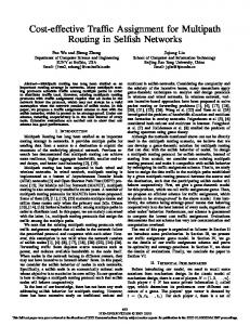
In the present section we compare the performance of coordinated multipath routing with parallel routing. For ease of exposition we assume only file transfers are present. This involves no loss of generality, since we could capture the influence of streaming traffic by redefining the cost function, as in Remark 1 above. The stability results of Theorem 1 provide stability conditions for multipath forwarding, as this fits in the general allocation framework (9-10). However we have not provided general stability results for parallel connections. We now give a counter-example which illustrates that, in general, the use of parallel, uncoordinated connections reduces the stability region. Consider the triangle network of Figure 1. Flows between any two pairs of nodes (say B-C) can go along the one-link route (B-C) between the nodes, or use the alternate two-hop route (BA-C). All three links are assumed to be of unit capacity. We denote by ρA the load to be carried from B to C, and call the corresponding file transfers type-A, and symmetrically ρB and ρC for file transfers of types B and C. Standard manipulations show that, when both direct and indirect routes

16

A

C

B

Figure 1: Example network where parallel uncoordinated connections lead to inefficiency are allowed, the capacity region is described by   ρB + ρC ≤ 2, ρ + ρA ≤ 2,  C ρA + ρB ≤ 2.

(41)

In the symmetric case when all three offered loads coincide, the stability condition reads ρ ≤ 1. In this case, stability can be achieved without using the alternate routes. Let us now see what happens when each file transfer uses two connections, one direct and one indirect. For definiteness assume that the allocation to each connection is α-fair, with equal weights for all connections. Let nA (resp. nB , nC ) denote the number of type-A (respectively, −B, −C) file transfers. Then file transfers of type i proceed at rate xi , i = A, B, C, where  1/α  1/α   1 1  = + , x A  p p +p    A 1/α  B C 1/α 1 + pA +p , xB = p1B C        1/α 1/α  1  xC = 1 + pA +p , pC B and the pi ’s are the Lagrange multipliers associated with the link capacity constraints. They are uniquely determined by   1/α  1/α  1/α  1 1 1  + n + n = 1, n B pA +pC C pA +pB  A pA    1/α  1/α  1/α 1 1 (42) + nC pA +p + nA pB +p = 1, nB p1B B C          1/α 1/α 1/α  1 1  + nA pB +p + n = 1. nC p1C B p +p C A C The fluid equations, in the case of symmetric loads, then read d ni (t) = ν − µxi (n(t)), dt 17

i = A, B, C.

(43)

We have the following: Proposition 3. Define ρ as λ/µ, and ρ∗ :=

1 + 2−1/α · 1 + 21−1/α

(44)

∗ The solution n(t) to the system of differential equations (43) diverges √ to infinity whenever ρ > ρ . In particular, when α = 2, the system is unstable provided ρ > 1/ 2 ≈ 0.71. Conversely, the solution n(t) decreases to zero in time at most θ[nA (0) + nB (0) + nC (0)] for a suitable constant θ > 0 whenever ρ < ρ∗ .

Proof: We shall rely on monotonicity properties of the allocations, which we summarise in the following lemma, the proof of which relies on elementary manipulations of (42), and is left as an exercise. Lemma 1. Assume nA ≤ nB ≤ nC . Then it holds that: pA ≤ pB ≤ pC ,

1/α

1/α

1/α 1 1 1 ≤ nB ≤ nC , nA pA pB pC

1/α

1/α

1/α 1 1 1 ≤ nB ≤ nC . nA pB + pC pA + pC pA + pB

(45) (46) (47)

We shall now deduce the following. Suppose nA ≤ nB ≤ nC . Then it holds that nA xA ≤ ρ∗ , where ρ∗ is defined in (44). Indeed, assume that it is not so, that is

1/α

1/α 1 1 + nA > ρ∗ . nA pA pB + pC Then, using the inequalities (45), we obtain that necessarily

1/α   1 nA 1 + 2−1/α > ρ∗ . pA On the other hand, (49) and the first equation of (42) imply that

1/α

1/α

1/α 1 1 1 ∗ + nB + nC < 1. ρ − nA pB + pC pA + pC pA + pB The sum of the two middle terms in the left-hand side is positive, by (47), so that

1/α 1 nC < 1 − ρ∗ . pA + pB 18

(48)

(49)

(50)

By (45), this further implies

nC

1 pC

1/α

< 21/α (1 − ρ∗ ).

In view of (46), this implies

nA

1 pA

1/α

< 21/α (1 − ρ∗ ) =

ρ∗ , 1 + 2−1/α

which contradicts (50), thus establishing the desired inequality (48). Thus, when nA ≤ nB ≤ nC , we necessarily have that d nA (t) ≥ µ (ρ − ρ∗ ) . dt Thus the minimum of the three components increases at rate µ(ρ − ρ∗ ), which establishes the first half of the proposition. The second half is established in a similar manner: by a direct adaptation of the argument used to establish (48) one can show that, when nA ≤ nB ≤ nC , the allocation xC is at least ρ∗ . Thus, the largest of nA , nB and nC decreases to zero at speed at least µ(ρ∗ − ρ), which establishes the second half of the proposition.
Remark 2. In the case where ρ < ρ∗ , the second half of the proposition, combined with Dai’s stability criterion [14] shows that the original stochastic system is ergodic. It can also be shown with additional work that the original stochastic system is transient under the assumption ρ > ρ∗ . We omit the detailed arguments in the present paper. Together, these results show that ρ∗ is indeed the exact capacity of the triangle network of Figure 1 under symmetric loads. As we have just seen, the use of parallel, uncoordinated connections can lead to strictly smaller capacity regions than coordinated multipath transfers. We now discuss a specific case of interest where the capacity region is the same for coordinated multipath and for uncoordinated parallel connections. Consider the case where each file transfer type r can use several paths p ∈ Pr , and each such path consists of a single link, as illustrated by Figure 2. The resources are then a collection of links, denoted by  ∈ L, and Γ (·) is the cost function associated with link . For definiteness, let us consider first sharp capacity constraints: Γ (x) = 0 if x ≤ C , and +∞ otherwise. As usual, denote by ρr the offered load due to type-r users. The stability condition, in this context, can be described in the following simple manner:

ρr < C , S ⊂ R, (51) r∈S

∈L(S)

where the subset of links L(S) is defined to be the union of the sets P(r) for all r ∈ S. Indeed, clearly the conditions with non-strict inequalities instead of strict ones are necessary for the existence of a feasible allocation of each load ρr to the links in P(r). The fact that these conditions 19

A

B

C

Figure 2: Example network with 1-hop routes: parallel unccordinated connections achieve maximal stability region are also sufficient is known as Hall’s theorem (see e.g. [5], p.77) in the case where the ρr and the C all equal 1. This extends (i) to integral loads and capacities by splitting each traffic source and link into components with unit capacity, (ii) to rational loads and capacities by rescaling, and (iii) to arbitrary positive loads and capacities by continuity. Denoting as usual by nr the number of type r-users, and by Ur the utility function used to determine their allocated rate via link , the allocation xr (n) to type-r users is then specified as
xr = xr , (52) ∈P(r)

where the xr maximise
r




nr

∈P(r)

Ur (xr ) −




 Γ 

∈L




 nr xr  .

(53)

r:∈P(r)

We now establish the following Proposition 4. Assume that for all links , and all user types r, s such that  ∈ P(r) ∩ P(s), the U
(x) is bounded away from zero and infinity, uniformly in x ∈ R+ . Then, under the stability ratio Ur

s
(x) condition (51), the solutions to the system of differential equations d nr (t) = νr − µr nr xr dt

(54)

 where xr is specified by (52–53) return to zero in time at most θ r∈R nr (0) for some suitable constant θ.  −1 Proof: Let W (t) = r∈S µr nr (t) denote the expected amount of work present in the system. We argue that, whenever W (t) > 0, it holds that d W (t) ≤ −, dt 20



where =

min

S⊂R,S=∅




∈L(S)

C −




 ρr  .

r∈S

Indeed, let R1 (t) denote the set of user types r such that nr (t) > 0. By the assumption of boundedness of the ratio of derivatives of utility functions, it holds that the capacity C of links  in L(R1 ) is entirely used by users of types r belonging to R1 . Thus, it holds that W (t + h) − W (t) = = ≤

 t+h 1r∈R1 (u) (ρr − nr xr (n(u)) du r∈R t   t+h    1 ρ − C R1 (u)=S S⊂R t r∈S r ∈L(S)  du  t+h − t 1R1 (u)=∅ du.



This establishes that W (t) decreases indeed at rate at least  until it reaches 0, concluding the proof.
Remark 3. Even for network topologies as in the previous proposition, where parallel connections achieve stability whenever synchronised parallel connections do, one may still prefer the latter allocation to the former. For instance, consider a single type of users, who can simultaneously access two resources, 1 and 2 , with associated cost functions Γ1 and Γ2 respectively. We know from the comments in Section 4.2.2 that, using coordinated multiple connections, the load ρ is at equilibrium split into ρ1 and ρ2 so that the cost Γ1 (ρ1 ) + Γ2 (ρ2 ) is minimised. In contrast, in the case of parallel, uncoordinated connections, based on respective utility functions U1 , U2 , at equilibrium the loads ρ1 and ρ2 are now specified by the fixed point equations in the variables:   ρ1 + ρ2 = ρ, ρi = nxi , i = 1, 2,   Ui (xi ) = Γi (nxi ) + βi , i = 1, 2, where βi is the Lagrange multiplier associated with the constraint xi ≥ 0 in the optimisation problem Maximise n [U1 (x1 ) + U2 (x2 )] − Γ1 (nx1 ) − Γ2 (nx2 ). Consider for instance the case where U1 (x) = U2 (x) = log(x), and Γi (x) = pi x, and assume p1 < p2 . In the coordinated case, we obtain ρ1 = ρ, ρ2 = 0, and a corresponding cost of ρp1 . In the uncoordinated case we obtain ρ1 = ρp2 /(p1 + p2 ), ρ2 = ρp1 /(p1 + p2 ) and a corresponding cost of ρp1 [2p2 /(p1 +p2 )], larger than the optimal cost by a factor of 2p2 /(p1 +p2 ). This illustrates the fact that, even when stability is not lost, lack of coordination can still be detrimental.

6

Second-order properties

The aim of the present section is to establish diffusion approximations for the rescaled Markov processes (L−1 Nr (t), L−1 Mr (t))r∈R of Section 3 around the fluid limits nr (t), mr (t), evolving 21

according to (24,25), that have been studied in Section 4. The derivations in this section are purely formal, and no rigorous justification is provided; we address the reader to [28] for a rigorous treatment of the single link scenario. This section is included for completeness and to illustrate how subtler performance issues could be addressed. We introduce the perturbation processes  ur (t) = √1L (Nr (t) − Lnr (t)) , vr (t) = √1L (Mr (t) − Lmr (t)) , together with the noise processes 1 ξi,r (t) = √ (Ξi,r (Lt) − Lt) , L

i ∈ {1, · · · , 4},

r ∈ R,

t > 0,

where the Ξi,r are the unit rate Poisson processes appearing in the representation (23). By taking ˆ , and m(0) = m, ˆ assuming differentiability of the allocation vector x with respect to the n(0) = n flow numbers nr , we obtain formally the limiting equations for the perturbation processes u, v: ur (T ) = ur (0) + ξ1,r (νr T ) − ξ2,r (νr T )   T T  ∂xr ˆ C) (us (t) + vs (t)) dt, (ˆ n + m; −µr 0 x ˆr ur (t)dt − µr 0 n ˆ r s∈R ∂n T s vr (T ) = vr (0) + ξ3,r (κr T ) − ξ4,r (κr T ) − ηr 0 vr (t)dt. Replacing the noise processes ξi,r by standard Wiener processes, we can alternatively write these as the following system of stochastic differential equations:  



√ ! u W1 2ν 0 !

µˆ x + µˆ n D µˆ n D  u  √ d , (55) dt + d =− 0

η 2κ 0 v v W2 where a represents the diagonal matrix with entries ar on the diagonal, D is the square matrix ˆ + m, ˆ and W1 , W2 are independent, standard |R|-dimensional with entries ∂xr /∂ns evaluated at n Wiener √ processes. In the above, for compactness of representation we have also replaced ξ1,r − ξ2,r by 2W1,r where W1,r is again a standard Wiener process, and similarly for ξ3,r − ξ4,r . This characterises the perturbation processes u, v as coupled Ornstein-Uhlenbeck processes. Correlations can then be determined from the matrices in the above representation. The matrix D is determined as follows, in the special case where Γ and U are twice differentiable. By differentiating ˆx ˆ , one obtains equation (22), denoting by H the Hessian matrix of Γ, evaluated at n ! U  (ˆ x) D = H ( ˆ x + ˆ n D) , so that

!#−1 " x) H ˆ x . D = − H ˆ n − U  (ˆ

(56)

For the sake of illustration, consider the case where Γ is as in (13), where the individual penalty functions Γj are twice differentiable. The Hessian matrix H then reads: ! H = AT γ  A 22

where the diagonal entry γj is given by 1  Γ Cj2 j



r

Ajr x ˆr (ˆ nr + m ˆ r) Cj

 .

Remark 4. By removing the m-component, that describes the streaming flows, in the above OrnsteinUhlenbeck process, which is formally done by setting κ and v to zero, we obtain a reduced OrnsteinUhlenbeck process for the fluctuations in the n-component. This is counter-intuitive, as one expects, from standard heavy traffic theory, the diffusion approximation of the m-component to behave like a reflected brownian motion instead. Such an expectation is backed by simulation results reported in [27]. However, the above Ornstein-Uhlenbeck process limit is obtained based on the assumption that the penalty function Γ is twice differentiable, whereas reflected Brownian motions in heavy traffic limits arise in the presence of sharp capacity constraints, hence non-differentiable Γ. These issues are investigated in greater detail in [28].

7

Conclusion

We have studied a flow level model of Internet congestion control, that represents the randomly varying number of flows present in a network. Bandwidth was assumed to be dynamically shared between file transfers and streaming traffic, according to a fairness criterion that includes TCP friendliness as a special case. Through the construction of an appropriate Lyapunov function we have established stability, under conditions, for a fluid model of the system. The presence of fairsharing streaming traffic results in a non-degenerate fluid model. Analysis of the model suggests that file transfers are seen by streaming traffic as reducing the available capacity, whereas for file transfers the presence of streaming traffic amounts to a simple modification in the network penalty function. While we have assumed that streaming traffic fairly shares the capacity with file transfers, our model can be adapted to the case where streaming flows have a minimum or fixed bandwidth requirement, and admission control is used so that the aggregate rate used by streaming traffic competes fairly with file transfers. For details see [27]. The general bandwidth allocation criterion we have considered encompasses balanced multipath routing, which could be implemented by modifying the existing TCP transport protocol as in the proposals of [20, 25]. We have also compared the performance of such routing to parallel, uncoordinated routing, which may be implemented with fewer changes to existing protocols. We have shown that the latter may strictly reduce the capacity region of the network as compared to the former. This strengthens the case for deploying modified versions of Internet transport protocols as those described in [20, 25]. Finally, we have formally identified second-order diffusion approximations to the first-order fluid limits of the number of flows in progress. These provide a basis for refined performance evaluation of integrated network-wide data transfer.

23

References [1] E. Altman, K.E. Avrachenkov and C. Barakat, TCP network calculus: the case of large delaybandwidth product, in Proceedings of IEEE Infocom, 2002. [2] N. Antunes, C. Fricker, F. Guillemin and P. Robert, Integration of streaming services and TCP data transmission in the Internet, In Proceedings Performance, 2005. [3] A. Bain and P. B. Key, Modelling the performance of distributed admission control for adaptive applications, Performance Evaluation Review, December 2001. [4] S. Ben Fredj, T. Bonald, A. Proutiere, G. Regnie, J. Roberts, Statistical bandwidth sharing: a study of congestion at flow level. In Proceedings of SIGCOMM 2001. [5] B. Bollobás, Modern Graph Theory, Springer, 2002. [6] T. Bonald and L. Massoulié, Impact of fairness on Internet performance. In Proceedings of ACM SIGMETRICS 2001. [7] T. Bonald and A. Proutière, On performance bounds for the integration of elastic and adaptive streaming flows, In Proceedings of ACM Sigmetrics / Performance 2004. [8] S. Boyd and L. Vandenberghe, Convex Optimization, Cambridge University Press, 2004. [9] P. Brémaud, Markov chains, Gibbs fields, Monte Carlo simulation, and queues. Springer-Verlag, New York, 1999. [10] L. Breslau, E. W. Knightly, S. Shenker, I. Stoica, and H. Zhang, Endpoint admission control: Architectural issues and performance. In Proceedings of SIGCOMM 2000, 57–69, 2002. [11] T. Bu and D. Towsley, Fixed Point Approximation for TCP behavior in an AQM Network. In Proceedings of ACM SIGMETRICS 2001. [12] C. A. Courcoubetis, A. Dimakis, and M. I. Reiman, Providing bandwidth guarantees over a besteffort network: call admission and pricing. IEEE INFOCOM, 459–467, 2001. [13] G. de Veciana, T-J. Lee and T. Konstantopoulos, Stability and performance analysis of networks supporting elastic services, IEEE/ACM Trans. on Networking 9, 2–14, 2001. [14] J. Dai, On positive recurrence of mutliclass queueing networks: a unified approach via fluid limit models, Ann. of Applied Probability 5, 49-77, 1995. [15] F. Delcoigne, A. Proutière and G. Régnié, Modeling integration of streaming and data traffic, Performance Evaluation 55 (3-4), 185-209, 2004. [16] S. Floyd and K. Fall, Promoting the use of end-to-end congestion control in the Internet. IEEE/ACM Transactions on Networking 7, 458–472, 1999. [17] Floyd, S., M. Handley, J. Padhye and J. Widmer (2000), Equation-based congestion control for unicast applications. In Proc. ACM SIGCOMM 2000, 43–54, Stockholm, 2000. [18] S. Floyd and V. Jacobson, Random early detection gateways for congestion avoidance, IEEE/ACM Trans. Networking, 4, 1993.

24

[19] R.J. Gibbens, S.K. Sargood, C. Van Eijl, F.P. Kelly, H. Azmoodeh, R.N. Macfadyen and N.W. Macfadyen, Fixed-point models for the end-to-end performance analysis of IP networks. 13th ITC Specialist Seminar: IP Traffic Measurement, Modeling and Management, Monterey, California, 2000. [20] H. Han, S. Shakkottai, C.V. Hollot, R. Srikant and D. Towsley, Overlay TCP for Multi-Path Routing and Congestion Control, submitted to IEEE/ACM Transactions on Networking. [21] IP monitoring project, Sprint labs. http://ipmon.sprintlabs.com [22] F.P. Kelly, Mathematical modeling of the Internet, in “Mathematics Unlimited - 2001 and Beyond” (Editors B. Engquist and W. Schmid). Springer-Verlag, Berlin, 685–702, 2001. [23] F.P. Kelly, P.B. Key, and S. Zachary, Distributed admission control. IEEE Journal on Selected Areas in Communications, 18, 2617–2628, 2000. [24] F. P. Kelly and A. K. Maulloo and D. K. H Tan, Rate control in communication networks: shadow prices, proportional fairness and stability, Journal of the Operational Research Society, 49, 237–252, 1998. [25] F. P. Kelly and T. Voice, Stability of end-to-end algorithms for joint routing and rate control, Computer Communication Review 35:2 5–12, 2005. [26] F.P. Kelly and R. J. Williams, Fluid model for a network operating under a fair bandwidth-sharing policy. Annals of Applied Probability 14 1055–1083, 2004. [27] P. Key, L. Massoulié, A. Bain and F. Kelly, Fair Internet traffic integration: network flow models and analysis, Annals of Telecommunications, 59, 1338–1352, 2004. [28] S. Kumar and L. Massoulié, Fluid and diffusion approximations of an integrated traffic model, Microsoft Research Technical Report MSR-TR-2005-160. Available at http://research.microsoft.com/users/lmassoul/MSR-TR-2005-160.ps . [29] S. Kunnyur and R. Srikant, End-to-end congestion control schemes: utility functions, random losses and ECN marks. IEEE INFOCOM, 2000. [30] T.G. Kurtz, Strong Approximation theorems for density dependent Markov chains, Stochastic Process. Appl. 6 223–240, 1978. [31] P. Kuusela, P. Lassila, J. Virtamo and P. Key, Modeling RED with Idealized TCP Sources, Proceedings of IFIP ATM & IP 2001, Budapest, Hungary, 155–166, 2001. [32] L. Massoulié and J. Roberts, Bandwidth sharing and admission control for elastic traffic. Telecommunication Systems 15, 185–201, 2000. [33] M. Mathis, J. Semke, J. Mahdavi, and T. Ott, The macroscopic behaviour of the TCP congestion avoidance algorithm. Computer Communication Review 27, 67–82, 1997. [34] J. Mo and J. Walrand, Fair end-to-end window-based congestion control. IEEE/ACM Transactions on Networking 8, 556–567, 2000. [35] R. Núñez-Queija, J.L. van den Berg and M.R.H. Mandjes, Performance evaluation of strategies for integration of elastic and stream traffic, In Proceedings ITC-16, 1999.

25

[36] J. Padhye, V. Firoiu, D. Towsley and J. Kurose, Modeling TCP Reno performance: a simple model and its empirical validation. IEEE/ACM Transactions on Networking 8, 133–145, 2000. [37] G. Raina and D.J. Wischik, Buffer sizes for large multiplexers: TCP queueing theory and instability analysis, In Proceedings of EuroNGI conference, Rome, April 2005. [38] T. Rockafellar, Convex Analysis. Princeton University Press, 1970. [39] M. Roughan, A. Erramilli and D. Veitch, Network performance for TCP Networks, Part I: persistent sources. In Proceedings of ITC’17 Brasil, September 2001. [40] R. Srikant, The Mathematics of Internet Congestion Control, Birkhauser, 2003. [41] Streaming Control Transmission Protocol. http://www.sctp.org

26