Proceedings of the 23rd UK Conference of the Association for Computational Mechanics in Engineering 8 - 10 April 2015, Swansea University, Swansea
Fluid-structure interaction with immersed boundary method based on hierarchical B-Spline based Eulerian grid *Chennakesava Kadapa, Wulf Dettmer, Djordje Peri´c Zienkiewicz Centre for Computational Engineering, Swansea University, Swansea SA2 8PP, UK. *
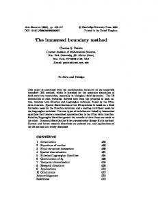
[email protected] ABSTRACT Fluid-Structure interaction (FSI) is a complex phenomenon and developing robust numerical schemes for studying FSI is quite a challenging task. The most widely used approach to simulate FSI is to use bodyfitted meshes with Arbitrary Lagrangian-Eulerian (ALE) formulation. However, fluid-mesh distortions due to the movement of solids limits the applicability of ALE formulation and also require efficient re-meshing algorithms. Creating good quality body-fitted meshes also adds to the difficulties associated with the ALE formulation. Immersed-boundary methods (IBMs) prove to be efficient alternatives in such scenarios involving large movements of solid bodies. In IBM fluid is solved on a regular cartesian grid on which the solid is free to move and as fluid mesh is independent of the movement of the solid there is no need for re-meshing algorithms. In the present work we propose IBM based on hierarchical B-Spline cartesian grid. One of the main motivating factors behind using hierachical B-Splines for the background fluid grid is their local refinement capability. The solution space, at the locations of steep gradients, can be enriched by the use of hierarchical B-Splines thereby eliminating the need to refine the whole grid. This results in significant savings in computational time. The immersed solid is represented by a set of Lagrangian points. The standard Galerkin formulation is used to discretise the governing equations and the unconditionally stable and second-order accurate generalised-α method is used for time-integration. Performance of the proposed formulation is demonstrated by studying several benchmark problems and comparing the parameters of interest with the reference values. The proposed method is applied to study the performance characteristics of a check-valve. This method proves to be efficient and robust in capturing topology changes during opening and closing of the valve. Without the need for any re-meshing algorithms and with the capability to perform local refinement the proposed formulation proves to be efficient and robust for simulating fluid-structure interaction phenomenon. Key words: Hierarchical B-Splines, Navier-Stokes, Immersed-boundary method, Fluid-Structure interaction. 1. Introduction to immersed boundary method The fundamental idea behind the immersed boundary method is that a solid-body, which is fixed/free to move is overlaid on top the fluid mesh as shown in Figure 1. The fluid mesh need not coincide with the boundary of the solid and hence there is absolutely no need for the body-fitted meshes used with ALE formulations. The methodology followed in the present work is more like the fictitious domain method of [3, 4, 5] than the immersed boundary method and its derivatives developed by Peskin [1]. In this work the Eulerian fluid grid is discretised with the hierarchical B-Splines because of their smoothness and localrefinement properties. The boundary of the immersed solid body is represented by a set of Lagrange points.
Ωf
Ωb
Γf
Γb
Figure 1: A solid body immersed on a fluid grid.
2. Hierarchical B-Splines B-Splines are piecewise-continuous polynomial functions which can be evaluated, for a given knot vector Ξ = {ξ0 , . . . , ξn+a+1 } and degree of polynomial a, by the relations, 1 if ξi ≤ ξ ≤ ξi+1 (1) Ni,0 (ξ) = 0 otherwise Ni,p (ξ) =
ξi+p+1 − ξ ξ − ξi Ni,p−1 (ξ) + Ni+1,p−1 (ξ) ξi+p − ξi ξi+p+1 − ξi+1
(2)
One of the important properties of the B-Spline functions is that a B-Spline function on a knot vector with knot span h can be evaluated as a linear combination of B-Spline functions defined on a knot vector with knot span h/2, as illustrated in Fig. 2. This hierarchical property of B-Spline functions is utilised to locally refine the areas of the fluid grid where steep gradients in the solution variables occur i.e., near immersed bodies. 1.0
1.0
0.8
0.8
0.6
0.6
0.4
0.4
0.2
Level - 0
0.2
0.0 0
1
2
1.0
0.8
0.8
0.6
0.6
0.4
0.4
0.0 0.0
1
2
3
1.0
0.2
Level - 1
0.0 0
0.2
0.5
1.0
1.5
2.0
0.0 0.0
0.5
(a) Q1
1.0
1.5
2.0
2.5
3.0
(b) Q2
Figure 2: Two-scale relation of the B-Spline functions.
3. Formulation for FSI Governing (Navier-Stokes) equations for the fluid: ρ
∂u + ρ(u · ∇)u − µ∆u + ∇p = f in Ω ∂t ∇ · u = 0 in Ω
(3a) (3b)
Governing equations for the rigid body: Ma + Cv+ Kd = F
(4)
u=v
(5)
Kinematic conditions at the interface: where, ρ, µ, u and p are the density, dynamic viscosity, velocity, and pressure of the fluid, respectively, and d, v, a, M, C and K are the displacement, velocity, acceleration, mass matrix, damping matrix and stiffness matrix of the rigid-body, respectively. Using a time-stepping scheme and after applying the weak form and Newton-Raphson method to solve the set of nonlinear equations 3, 4 and 5, yields the following the matrix system, Ru du¯ Kuu Kup Kuλ 0 K 0 0 0 dp¯ R p pu (6) = − K ¯ R 0 0 K d λ λ λu λv R 0 0 K K dv¯ vλ
vv
v
where, λ are the Lagrange multipliers to impose the kinematic interface condition 5 at the immersed points.
4. Numerical examples Equal-order interpolation with quadratic (Q2 ) B-Splines without any stabilisation is used in all of the examples presented here. Even though this velocity-pressure combination is unstable the results obtained are found to be extremely encouraging. Dirichlet boundary conditions on the fluid domain are applied using penalty approach. 4.1. Flow over an elastically mounted square - galloping Galloping is aerodynamically unstable phenomenon involving oscillations of high amplitudes. The fluid domain, boundary conditions and hierarchical B-Spline mesh are as shown in Fig. 3. A rigid square body supported on a spring-mass-damper system is exposed to fluid flow. The properties of the spring-massdamper system are: K = [3.08425], C = [0.0581195] and M = [20.0]. And the density and viscosity of the fluid are ρ = 1.0 and µ = 0.01, respectively. The side of square is D = 1. The problem is studied with a staggered scheme for Reynolds numbers upto Re = ρDu1 /µ = 250, by varying the inflow velocity. The amplitudes of oscillation of the the rigid-body for different Reynolds numbers are shown in Fig. 3(c) along with the reference values obtained with body-fitted meshes with ALE formulation [2]. The graph illustrates that the phenomenon of galloping is captured very well. u2 = 0, t1 = 0 15
2.0
u1 = us u2 = 0
Present Ref
1.5
1.0
p=0
1
0.5
15 0.0
u2 = 0, t1 = 0 10
−0.5 0
20
(a) Geometry, boundary conditions
(b) HBS mesh
50
100
150
200
250
300
(c) Amplitude Vs Reynolds number
Figure 3: Galloping of a square. DOF = 34314 (fluid) + 160 (points) = 34474.
4.2. Simulation of a check-valve in operation In this example we demonstrate the performance of a check-valve under varying inflow conditions. The geometry, boundary conditions and the hierarchical B-Spline mesh used for the simulation are as shown in Fig. 4. The length of the domain is taken as L = 200 mm. Because of the symmetry only a half portion is modelled. The density and viscosity of the fluid are considered to be ρ f = 792 kg/m3 and µ f = 0.008 Ns/m2 , respectively. The valve is assumed to be a rigid-body supported by a spring-mass system and is modelled as a line. The mass and stiffness of the spring-mass system are m = 3.52 × 10⁻⁵ kg and k = 380.0 N/m, respectively. The inlet pressure varies sinusoidally given by the relation pin = p sin(2π f t) and the outlet pressure is pout = 0. The contact between the two rigid bodies is modelled using Lagrange multiplier approach. The problem is solved using the monolithic scheme because of the added-mass issue and 100 time-steps per time period is used. The displacement of the valve in response to the varying inlet pressure shown in Fig. 5 illustrates that opening and closing of the valve are captured extremely well. It can also be observed that, for the given magnitude of inlet pressure, the valve ceases to operate as the frequency of the inflow is increased. This is in line with the expected behaviour. 5. Conclusions We presented an efficient immersed boundary method based on hierarchical B-Spline cartesian grid for the numerical simulation of fluid-structure interaction problems. The numerical examples presented demonstrate the robustness of the proposed method. The local refinement capability of the hierarchical B-Splines makes the proposed method extremely efficient as it results in fewer number of degree of freedom.
pout
4.4 mm L
11.5 mm
40 mm
3 mm
vx = 0 vy = 0
vx = 0 vy = 0
pin 83 mm
(a) Geometry, boundary conditions
(b) HB-Spline mesh
(c) Mesh around the opening
Figure 4: Check-valve simulation: Symmetric boundary is considered on the right edge. DOF = 29001 + 48 + 2 = 29051. 2.0
f=10 Hz f=25 Hz f=100 Hz
Displacement (mm)
1.5 1.0 0.5 0.0 −0.50
1
2 3 Nondimensional time (t/T)
4
5
Figure 5: Check-valve simulation: Response of the valve for inlet pressure, pin = 6 sin(2π f t).
References [1] Peskin, C.S., The immersed boundary method, Acta Numerica, Vol.11, pp. 479-517, 2002. [2] Dettmer, W.G., Finite Element Modelling of Fluid Flow with Moving Free Surfaces and Interfaces Including Fluid-Solid Interaction, PhD thesis, Swansea University, 2004. [3] Diaz-Goano, C. and Minev, P.D. and Nandakumar, K., A fictitious domain/finite element method for particulate flows, Journal of Computational Physics, Vol.192, pp. 105123, 2003. [4] Glowinski, R. and Pana, T.-W. and Hesla, T.I. and Joseph, D.D., A distributed Lagrange multiplier/fictitious domain method for particulate flows, International Journal of Multiphase Flow, Vol.25, pp. 755-794, 1999. [5] P.T. Baaijens, F.P.T., A fictitious domain:mortar element method for fluidstructure interaction, International Journal for Numerical Methods in Fluids, Vol.35, pp. 743761, 2001.