FMS Cyclic Scheduling with Overlapping production cycles Ouajdi KORBAA, Hervé CAMUS, Jean-Claude GENTINA Laboratoire d’Automatique et Informatique industrielle de Lille (L.A.I.L.) E.C. Lille - L.A.I.L. URA CNRS 1440 Cité Scientifique, B.P. 48, F-59651 Villeneuve d’Ascq CEDEX Tel : (33) 20.33.54.04 Fax : (33) 20.33.54.18 E-mail :
[email protected] [email protected] [email protected]
Abstract We are interested in the determination of the command of Flexible Manufacturing Systems (FMS) under small or medium production. We have chosen the Cyclic Behavior to reduce the complexity of the general scheduling problem. In this paper, we recall and discuss the most known cyclic scheduling heuristics. The aim is to combine their advantages and give a new heuristic to determine a cyclic command which can reach the optimal production speed while minimizing the Work in Process (W.I.P.). In fact we want to minimize the W.I.P. to satisfy economical constraints. The aim of this paper is to formulate the general cyclic scheduling problem. That’s why we consider overlapping production cycles. The obtained command is modeled by a marked graph and represented by a Gantt diagram with both resources and pallets points of view.
1. Introduction As part of the control of FMS, subject to small or medium demand, we have studied the problem of the command by developing predictive approach to compute a cyclic and deterministic schedule. This repetitive command has to be optimized as regard with the criteria we choose : it has to minimize the makespan while minimizing the number of pallets (transport resources) for evident economical reasons and the cyclic production horizon (number of part types to produce each cycle) in order to simplify the computation of the command. That is why, in Camus [1], we have presented a stepwise and structured method for performance evaluation of the production system. The problem we will focus in this paper is to determine an algorithm for the computation of a cyclic schedule respecting a hard constraint which is the optimal cycle time CT and trying to minimize the Work in Process. We can find in the literature several scheduling heuristics such as Erschler et al [9], Hillion et al [10], Valentin [14], Ohl et al [12], ... The problem is that these algorithms
are either concerning different assumptions or using different optimizing criteria or introducing artificial constraints which prevent them to reach the optimal solution. In section 2, we give some basic definitions and main assumptions about FMS modeling with Petri Nets and cyclic schedules. Then, in section 3, we recall and discuss the existing cyclic scheduling methods. In section 4, we present and justify a new heuristic. Finally a conclusion and some extensions are given in section 5.
2. Some Definitions and Assumptions We suppose the reader familiar with a modeling tool of the discrete event systems : the Petri Nets and its main properties, presented for instance in Murata [11]. The first assumption we make is that the operating times are deterministic because we want to study the behavior of the system and to compute a predictive command. An important sub-class of Timed Petri Nets are Timed Event Graphs in which each place has exactly one input and one output transition and for which all weights associated to arcs are equal to one. This Petri Net can perfectly modelize the command (dynamic behavior) we want to implement. At the end of the optimization approach we have obtained a model where all the operating sequences are linear and it remains to compute the optimal schedule. This last step consists of linking the transitions by circuits which determines the order in which a resource will carry out the operations. Hillion [10] had shown that there are three types of circuits in such a Marked graph : (i) process circuits with tokens modeling the products, (ii) resource circuits with one token per circuit modeling a machine, (iii) hybrid or mixed circuits which contain parts of circuits of type (i) and (ii). There are some other important results concerning Timed Event Graphs and their circuit-based analysis : Commoner et al [7] have shown that a strongly connected event graph is live if and only if each elementary circuit is marked. Furthermore, the number of tokens in each circuit remains constant, which means that each circuit γ corresponds in fact to a P-semiflow. Ramamoorthy et al [14] associates to each elementary circuit γ of type (i), (ii) or (iii) these characteristics : µ( γ ) =
∑ D( t) , the sum of all transition timings of γ
∀t ∈γ
M( γ ) (= M 0 ( γ )) , the (constant) number of tokens in γ C(γ) = µ(γ)/M(γ), the cycle time of γ. It has been shown that, after a finite transient period and using the firing semantics “fire an enabled transition as soon as possible”, the maximum speed at which the net will work in steady state is given by : C* = Max (C(γ)) for all circuits of the net.
At the previous step, we have defined CT as the minimal cycle time associated to the maximal throughput of the system we want to respect : CT = Max (C(γ)) for all resource circuits = C* Then we have to make sure that all circuits of type (i) and (iii) are faster than CT. The two factors influencing their speed are : (a) the number of tokens in circuits (i) (b) the choice of circuits (ii) (sequencing of the resources) which determines circuits (iii) We assume that : - products remain clamped to their transport resource (pallet for example) during their entire sojourn in the FMS, - empty transport resources are reloaded with raw parts as soon as possible. The last two assumptions allow us to treat equally the maximum W.I.P. we want to minimize and the number of transport resources in the system. We suppose, also, that the previous performance evaluation step kept only three indeterminisms : the transport system flexibility (regrouping the operating sequences), the shared resources (operation sequencing on the machines) and the W.I.P. (number and initial position). Also, the cyclic production horizon (number of part types to produce each cycle) is already fixed in a previous planning step, see Camus [2]. Hence we know the optimal cycle time and we must respect it in the final schedule. Moreover the operating sequences are linear (no flexibilities) so we can compute the lower bound of the number of pallets to respect the cycle time CT (necessary but not mandatory sufficient) :
∑ operating time O.S. to be carried by i * B= ∑ CT pallets type i
For a better comprehension of the following sections we introduce an illustrative example, see Valentin [15]. Two part types (P1 and P2) have to be produced on three machines U1, M1 and M2.
* The symbol x means the first integer superior or equal to x
The first part type contains three operations : U1(2 t.u.) then M1(3 t.u.) and M2(3 t.u.). The second one contains 2 operations M1(1 t.u.) then U1(2 t.u.). The production horizon we use in this study is fixed and equal to E={3P1, 2P2}. Hence in each cycle we have to produce 5 parts with the production ratios 3/5 and 2/5. We suppose that there are two kinds of pallets : pallets dedicated to the part type P1 and pallets dedicated to the part type P2. Each transport resource can carry out only one part type. The operating sequences of each part type are denoted respectively OS1 and OS2. The Petri net model contains the operating sequences corresponding to P1 and P2 duplicated 3 and 2 times to respect the production horizon. It is a FRT-net, see Campos [4] for the definitions and the main properties. e0 1/5
1/5
OS1
t11
e1 Ptr(P1)
M1
(3)
U1
t12
M2
U1
M1
t12
M2
1/5 OS2
t21
M1
(1)
M1
(3)
t13 (2)
t11 (2)
(3)
t13 (2)
t11 (2)
t12
1/5 OS2
OS1
U1
(2) tf
1/5
OS1
t13
M2
(2)
U1 M1 M2
Figure 1 : Illustrative example
M1
(1)
t22 (2)
t21
U1
t22 (2)
U1
Ptr(P2) e2
From the performance analysis we obtain the bottleneck machine (M1) and an optimal cycle time CT equal to 11 t.u. Of course in this step we assumed that we have enough parts (e0) and pallets (e1, e2) to consider only the machines P-semiflows for computation of the bottleneck resource. The final scheduling needs at Ohl et al [12], as defined below : ∑ Operating Times of OS P1 B= CT
least B pallets to respect the optimal cycle time, see
∑ Operating Times of OS 21 6 P2 + = + =3 CT 11 11
3. Some scheduling algorithms Now we’ll present the three scheduling heuristics and the obtained schedules in order to compare them. We will also bold the interesting definitions and characteristics. In section 4, we will combine these points to make a new heuristic. All the methods offer to give a schedule which respects the horizon and the optimal cycle time.
3.1 Hillion’s Heuristic The problem solved in Hillion et al [10] is related with the optimization of the control circuits of the system, while the process circuits are known. Each process circuit is composed of only one operating sequence. Each pallet is supposed dedicated to only one operating sequence (process circuit). The Hillion’s heuristic is based on the progressive and parallel placing of the operations belonging to the « next operation to do » from all the operating sequences. It runs a placing function to choose in this set the operation to place definitely. Then we iterate the process till placing all the operations. Let rj be the number of remaining cycle times for the process j (if this number is superior than the initial expected number then it is equal to zero).
(
)
At j = 1 + r j * CT − {end date of the last scheduled operation on process j} is the Available time of the process circuit j. Let Ro j =
∑ ( ) , the sum of remaining operating times in the process j
D t jk k ∈remaining operations
also called remaining workload of the process j.
Ro j . This function translates the degree The criterion is a cost function : d j = 1 − At j of freedom of an operating sequence. Indeed the greater it is the smaller the remaining workload is compared to the available time. In spite of this criterion the heuristic can sometimes (when Atj is negative) end at a « non feasible schedule » because the next operation to do can’t be placed at all : neither with the current W.I.P. nor with an extra one. The Hillion’s wiliness consists on relaxing the constraint of the minimal cycle time by increasing it « temporally » and restart the resolution. The process can be repeated until obtaining a schedule. As the aim of the method is to respect the optimal cycle time, the obtained W.I.P. isn’t satisfactory (because it corresponds to a non minimal cycle time). So The algorithm memorizes the computed resource circuits and re-computes the W.I.P., with a heuristic, to minimize it while respecting the optimal cycle time of the shop.
Part type W.I.P. P1 W1 P1 W2 P1 W3 P2 W4 P2 W5 W6
op12 op11 op13
op13 op12 op11
op11 op13 op12 op22
0
op21 op22 op21
time
11 Figure 2 : Hillion's schedule
Hence, the Hillion’s scheduling method takes place in two phases. The first one consists in the computation of the sequencing of the operations on the machines. It clears on a Marked Timed Event Graph. The second one undertakes to take off the tokens and executes a minimization of the W.I.P. which requires the computation of all the minimal circuits. The final schedule has a cycle time equal to CT (the optimum) and needs 6 pallets, M1 remains the critical resource . We note that each operating sequence uses its own pallets.
3.2 Valentin’s Heuristic The main inconvenient of the above method is that it doesn’t take into account the machines constraints. Indeed the degree of freedom is only function of the remaining operating time and the available time of the operating sequence. That’s the reason for which Valentin tried to repair by associating to each machine the set of resource available intervals such as each interval is bigger than the smallest remaining operation. Therefore each one of these intervals can contain at least one of the remaining operations. This criterion allows the heuristic to give a better schedule than the last one i.e. the obtained W.I.P. decreases, see Figure 3. Indeed, the obtained schedule requires 5 pallets to work at maximum speed instead of 6 with the Hillion’s method. So, the Valentin’s heuristic works with the same principle than Hillion’s heuristic i.e. two stages to compute a schedule : the computation of the entry sequence and if necessary the minimization of the W.I.P. Besides the inconvenient of dividing the scheduling problem into two sub-problems, which adds constraints to the resolution and can prevent obtaining the optimal solution, one other problem concerns the placing function. Ro j ), we can notice that in Indeed, while studying the cost function ( d j = 1 − At j several cases, when the end of the last placed operation coincides with the end of a cycle, the denominator is equal to zero and appears then a « dividing by zero » problem (when Atj is equal to zero : it occurs in the particular case when the end of last placed operation coincides with the date CT of the pallet number
(1+ r ) ). j
Part type W.I.P. P1 P1 P1 P2 P2
op12 op11 op13
W1 W2 W3 W4 W5
op13 op12 op11
op11 op13 op12
op22
op21 op22
0
op21 11 time
Figure 3 : Valentin's schedule
In addition, even if the criterion takes into account the machines, there is only one cost function to take into account two different problems : the minimization of the W.I.P. and the respect of the cycle time.
3.3 Ohl’s Heuristic The first difference, in comparison with the last heuristics, is the starting point. Indeed, instead of scheduling each operating sequence alone, it keeps the possibility of regrouping some operating sequences, using the same type of pallets. Hence each pallet will be dedicated to one or many O.S. We may, of course, try all the possible regroupings to obtain the best possible solution. We wont describe all the possibilities of regroupings but we present, directly, the regrouping giving the best schedule, see Figure 4. We remind, once again, that the approach requires the whole run of the search space in order to get the best possible solution. The best regrouping model, Figure 4, contains two process circuits R1 and R2. R1 is made of all the operating sequences supporting the same type of pallets P1 :(three operating sequences OS1) as for R2, it contains the operating sequences needing the second pallets type (two operating sequences OS2). There is only one way to regroup the O.S. inside each regrouping because they are all identical. In the general case, for each partition of O.S., we have to test all the cyclic regrouping (precedence constraint between the operating sequences using the same pallets) to be sure to get the best solution. The second interest of this method is the cost function. Indeed the placing function is based on two criteria, which is logical because we have two constraints : the cycle time and the W.I.P. Let RTM[i] be the maximum time of resource i. Let RTT[i] be the remaining operating time for resource i. CT-RTM[i] will denote the available time for the resource i. RMM[i] = CT - RTT[i] - RTM[i] is the remaining slack time of resource i. This function relates the respect of the cycle time and shall never be negative unless the schedule will be non feasible. This term has been defined to guarantee a schedule in only one run. Indeed, during the computation, while RMM[i] isn’t negative, we are sure that the schedule is admissible and without any problem of « dividing by zero ». The second criterion is a real cost function. It depends on the remaining slack time of the resource, the remaining slack time of the process and especially the current W.I.P. to reply to the W.I.P. optimization requirement.
The Ohl’s heuristic is based on a progressive placement of the operations. In each iteration the placing function draws the operations sequence with the minimal cost and places the first operation(s) of this sequence.
t11
U1
(2)
t11
U1
(2)
t12
M1
(3)
t12
(2)
M2
U1
(2)
M1
(3)
t13
t11
t12
M2
M1
(1)
M1
(3)
t13
t21
t13
M1
(1)
t22 (2)
t21
U1
t22
U1
(2)
M2
(2)
(2)
Regrouping R1
Regrouping R2 U1 M1 M2
Figure 4 : Cyclic regrouping 1. We try to schedule this operation as early as possible in the current W.I.P. of the corresponding regrouping. 2. This placing creates a time ∆ of resource unuse (∆ positive or null). So we compute the remaining slack time of the resource. 3. If the remaining slack time of the resource is usually positive or null then we are sure that the current schedule is still admissible so we go to the next iteration.
4. If the remaining slack time of the resource is negative we can say that the resource was unused too much so we have to schedule the operation as early as possible for the machine. Hence we add a W.I.P., we loose a little remaining slack time of the process but we keep the same remaining slack time of the machine and we are sure that the scheduling is still admissible so we go to the next iteration. We notice that with this method the scheduling is obtained in one run, that it respects both optimal cycle time and horizon and that it takes into account both processes and resources. The last point appears in the cost function and mainly in the Gantt diagram, see Figure 5. This diagram is composed of two diagrams, one for the machines availability and the other, less original and more known than the first, for the actual scheduling. regrouping process M M
1 1
2 1
W.I.P. W1 W2 W3 machines U1 M1 M2
op12 op13 op22
op11 op21
op22 op12 op13
op11 op21 op13
op13
op11 op12
op12 op13 op22
op11 op21 time
op11 op12
0
op22 op12 op13
op11 op21 11
time
Figure 5 : Ohl’s schedule The obtained scheduling is said with unrelated cycles. That means that any operation must start and finish in the same cycle. The result is perceptibly better than the previous methods. Indeed, it needs 3 pallets (the minimum required) instead of 6 for Hillion’s and 5 for Valentin’s. This can be explained by the fact that Ohl’s heuristic is less constrained.
4. The new Algorithm Nevertheless, even if it reaches the optimal W.I.P. for the following example, Ohl’s heuristic can be improved. Indeed two weaknesses remain in the heuristic. The first one is the fact that if, at an iteration of the algorithm, an available resource interval is created, there is no way to recover it and it is lost for the following iterations. As for the second, it is the unreleased cycles scheduling. Considering the cyclic aspect of the command, it is strange that neither of the precedent heuristics (including Ohl’s) tried to schedule with overlapping cycles because nothing can prevent an operation to begin in a given cycle and finish in the next one.
Actually the precedent problem results directly from the Petri net modeling and it is a fact that we have some problems to model the final Event Graph. However we shouldn’t introduce artificial constraints. Hence we propose to give a new cyclic scheduling heuristic with overlapping cycles and to show the interest compared to Ohl’s heuristic.
4.1 The problem characteristics Let’s recall the critical features that are printed out in our heuristic : 1. Cyclic regrouping of the operating sequences. 2. The schedule is obtained in one run. 3. The operations placing must be progressive and parallel (concerns all the process circuits at the same time). 4. A cost function computes, at each iteration, the next operation to do. 5. This cost function takes into account the W.I.P. and the remaining slack time of both the processes and the resources. 6. A placing function decides the placing policy to choose. 7. The possibility of recovering the resource available intervals. The last point needs some explanations because we noticed a slight problem in Valentin’s definition of the available intervals. Let’s consider the following example to explain this problem : we suppose that we have a cycle time equal to CT and that we have already scheduled one operation O with an operating time equal to T at date t1 such as 0 < t1