Focusing ATMS Problem-Solving: A Formal Approach

Department of Computer & Information Science

Technical Reports (CIS) University of Pennsylvania

Year 1992

Focusing ATMS Problem-Solving: A Formal Approach Teow-Hin Ngair

Gregory Provan

University of Pennsylvania

University of Pennsylvania

This paper is posted at ScholarlyCommons. http://repository.upenn.edu/cis reports/299

Focusing ATMS Problem-Solving: A Formal Approach MS-CIS-92-61 GRASP LAB 326

Teow-Hin Ngair Gregory Provan

University of Pennsylvania School of Engineering and Applied Science Computer and Information Science Department Philadelphia, PA 19104-6389

July 1992

FOCUSING ATMS PROBLEM-SOLVING: A FORMAL APPROACH Teow-Hin Ngair

Gregory Provan

Computer and Information Science Department University of Pennsylvania Philadelphia PA, 19104-6389, USA Abstract T h e Assumption-based Truth Maintenance System (ATMS) is a general and powerful problem-solving tool in AI. Unfortunately, its generality usually entails a high computational cost. In this paper, we study how a general notion of cost function can be incorporated into the design of an algorithm for focusing the ATMS, called B F ATMS. T h e BF-ATMS algorithm explores a search space of size polynomial in the number of a,ssumptions, even for problems which a.re proven t o ha,ve exponential size labels. Experimental results indicate significant speedups over the standard ATMS for such problems. In addition t o its improved efficiency, the BF-ATMS algorithm retains the multiple-context capability of an ATMS, and the important properties of consistency, rninimality, soundness, as well as the property of bounded completeness. T h e usefulness of the new algorithm is demonstrated by its application t o the task of consistency-based diagnosis, where dramatic efficiency improvements, with respect t o the standard solution technique. a.re obtained.

INTRODUCTION The ATMS is a useful and powerful general problem-solving tool which has been widely used within AI. The range of applications include nonmonotonic reasoning [McCarthy, 1980; Reiter, 1980], qualitative physics [Forbus, 19901, visual interpretation [Bodington et al., 1990; Provan, 1990bI and diagnosis [de Kleer et a)., 1990; de Kleer and Williams, 1987b; Reiter, 19871. The ATMS allows search to be simultaneously conducted on multiple contexts, where each context (also known as environment) defines a set of assumptions about the problem domain. However, this flexibility comes at the cost of a high overhead due to storing many (and sometimes exponentially many) sets of such assumptions. Controlling the problem solver does not alleviate the poor performance on many tasks, such as diagnostic reasoning [Reiter, 19871, as it is the ATMS's generation of an enormous number of environments which is often the cause of inefficiency [Provan, 1990~1.Moreover, it is not always necessary to compute all environments for some domains, such as dia.gnosis. Various methods have been proposed to focus the ATMS on certain subsets of the search space (e.g. [Dressier and Farquar, 1990]), but none have been both general and effective. The goal of this study is to analyze the efficiency of the ATMS in solving problems in several domains, and devise efficient algorithms for problems the standard ATMS does not solve efficiently. A cost-function-based algorithm has produced significant efficiency improvements in the ATMS, as has been demonstrated for the domain of diagnostic reasoning. This paper provides a coherent semantics for both the ATMS label representation and the ATMS algorithms. In addition, the use of cost. functions for focusing is directly integrated into the ATMS algorithm; the semantics of this extension of the ATMS are simply and precisely defined. The cost-function approach, although not new to the A1 literature, has not been rigorously applied to ATMS-based problem solving to date. We present a simple theoretical framework for a cost function p (and associated order one hour6

Table 2: Example run of BF-ATMS with various bounds One can observe that the BF-ATMSalgorithm has enabled us to generate the ATMS labels in an incremental fashion and the algorithm terminates rather rapidly for a low cost bound. However, the simple cost function is not very helpful in efficiently finding the minimum cost environments for all the nodes in our example, because the cost of every environment in the node b: is 16. But we can solve this problem by changing the cost function to indicate the preference of choosing assumptions of type A instead of type B. In particular, we can assign to each assumption the cost of 1 if it is of the form A,, otherwise, the cost of 100. The sum of assumption costs is then used as the cost of an environment. With this modified cost function, the BF-ATMScan compute a minilnum cost environment for every node in less than 0.2 second. With exactly the same cost function, albeit not a very efficient one, we can also generate an even parity and several odd parity 20-bit strings in about 0.5 second and 3 seconds respectively. In conclusion, the selection of a good (but not necessary the best) cost function for the given problem is essential for deriving the desirable solutions in a reasonable amount of time. The question is: what type of cost function would induce the assignment of an ordering over the environments to guarantee polynomial performance in the ATMS? To ensure polynomial-time performance, no more than a polynon~ialnumber of environments can be explored. Since environments are constructed beginning with the empty environment {) and incrementally following the cost ordering, a good cost fiinction for a problem is therefore one that induces a metric with the property that an acceptable solution set is a t polynomial (with respect to the size of assumptions) distance away from the empty environment. In many applications, we know a pr701-1 some characterization of the solution sets. For instance, we may know that at least one solution set comes froill a small subset of assuinptions; or there exists a solution environment with less than 1 assumptions. Consequently, good cost functions can be designed accordingly: 1. e ( p ) = 0 if p

A', co otherwise;

where the assumption sets is A , the snla.11 subset of assuillptions is A' C A , and p C A is any environment. Observe that the combination of these cost functions with the BF-ATMS algorithm subsume the focusing strategies described in Section 5.

8

DIAGNOSIS FROM FIRST PRINCIPLES

In [Reiter, 19871, Reiter described an algorithm for generating diagnoses in which conflicts of a system are generated incrementally. At each stage, one computes the hitting sets of the conflicts t o find possible diagnoses of the system. However, missing in the paper is an efficient conflict generator. In addition to being an efficient (minimal) conflict generator, the BF-ATMS algorithm can also be used as an efficient consistency checker (see Section 3). In the following, we describe a diagnostic algorithm in which the BF-ATMS algorithm plays an important role. As a motivating example, consider the circuit in Figure 1. Notice that the number of conflicts is 2n even though there are only 2n 1 kernel diagnoses. Using a cost function similar to the above, one can efficiently find a conflict. On the other hand, to find the entire set of conflicts would have taken too much time. This clearly demonstrates that it is not a good idea for any diagnostic system, e.g. GDE [de Weer and Williams, 1987b] and Sherlock [de Kleer and Williams, 19893, to take the approach of first generating the entire or a large collection of conflicts before the generation of diagnoses. The following are the formal definitions relevant to our study of diagnosis. Most of them are borrowed directly from [de Kleer et nl., 19901.

+

Definition: A system is a triple a SD,

(SD, COMPS, OBS)

where:

the system description, is a set of first order sentences;

a COMPS,

OBS,

the system components, is a finite set of constants;

a set of observations, is a finite set of first order sentences.

Definition: An AB-literal is AB(C),or TAB(^) for some

cE

An AB-clauseis a disjunction of AB-literalscontaining no complementary pair of AB-literals. A conflict of (SD, COMPS, OBS) is an AB-clauseentailed by SD U OBS. A minimal conflict is a conflict where no proper subset of it is a conflict. COMPS.

We will adopt a result (Corollary 1 ) from [de Kleer et al., 19901 as our definition of kernel diagnosis:

Definition: The kernel diagnoses of (SD,COMPS,O B S ) are the prime ilnplicants of the minimal conflicts of SD U OBS. Note that the prime irnplicants of the nliniillal conflicts a.re precisely the minimal hitting set of the minimal conflicts, i.e. the sma,llest sets in the cross product of the minimal conflicts. One usually multiplies the minimal conflicts in a.n i?zcrem.entalfashion in deriving the desired kernel diagnoses. The following definition a.llows us to describe such a process more precisely:

Definition: An incomplete diagnosis is a subset of a diagnosis. The expansion of an incomplete diagnosis p by a conflict C is the set of new incomplete diagnoses {p U {c) I c E C}, while the process of deriving this set is called expandi~zgthe incomplete diagnosis p by C.

The process of generating diagnoses as described in [Reiter, 19871 is to: (1) start from the empty set as the only incomplete diagnosis, and ( 2 ) replace elements in the collection at each step by their expansions (with some suitable conflicts), until we obtain the desired diagnoses. Using essentially the same approach, we consider the following algorithm for generating kernel diagnoses : Procedure

GEN-DIAG

1. Check if the current ATMS is consistent. If so, report that the only kernel diagnosis is the empty set and quit.

2. Initialize the incomplete diagnoses database t o contain the empty list as the only element.

3. Retrieve an element p from the incomplete diagnoses database. If none exists, then quit. 4. Generate a minimal conflict

C.

5 . Consider every element in the expansion of p by C.If it is consistent with the system, insert it into the diagnoses databa.se, otherwise insert it to the incomplete diagnoses database. 6. Repeat from step 3. In this discussion, we will only be interested in systems that can be encoded in finite propositional Horn clauses for which we have an efficient conflict generator and consistency checker. In particular, in an actual implementation of the above algorithm, the BF-ATMS algorithm is used to check both the consistency for verifying a diagnosis and to generate a conflict for expanding an incomplete diagnosis. Note that the conflict returned by the BF-ATMS algorithm is always minimal. A major difference between the GEN-DIAG algorithm and Reiter's HS-tree algorithm is that for each expansion of an incomplete diagnosis, we generate a new minimal conflict. This contrasts with using the same conflict to expand every incomplete diagnosis in Reiter's approach. At first glance, this appears to be a more expensive approach. But there are several reasons why we do this. In particular, we have a conflict generator which generates minimal conflicts with great efficiency. Furthermore, as we shall see later, we can focus the ATMS t o return a good conflict for each incomplete diagnosis so that the search space for the diagnoses can be greatly pruned. Another important reason is that this incremental fashion of expanding incomplete diagnosis allows us to incorporate a cost function into the system so that lower-cost kernel diagnoses can always be generated before the consideration of the higher-cost ones, as in the case of label generation in the BF-ATMS algorithm. From the definition of kernel diagnosis, we know that the G E N - D I A G algorithm will eventually find all the kernel diagnoses of the syqtem. However, Inany improvements to it are needed to make it efficient. First, we need only to maintain a minimal set of incomplete diagnoses, i . e . all incomplete diagnoses that are subsumed by another incomplete diagnoses can

be deleted from the incomplete diagnoses database. This is because every kernel diagnosis that will be generated (via expansion) by an incomplete diagnosis will also be generated by a smaller incomplete diagnosis. Similarly, since we are only interested in kernel diagnoses, we need only to maintain a minimal set of diagnoses in the diagnoses database. Therefore, the insert operation in step 5 of the above procedure should delete elements in the database which are subsumed by the new element or discard the new element if it is subsumed by an existing element. A second improvement for the procedure can be derived from the observation that many conflicts generated in step 4 may not contribute to the process. In particular,

Proposition 10 Suppose p is an incomplete diagnosis, if p C S COMPS,then 5 is a diagnosis of (SD,COMPS,OBS) if, and only if, 6 - p contains a hitting set of the set of conflicts S, that has empty intersection with p. In addition, S is kernel only if S - p is a minimal hitting set of S,. Proof: (=+) Given that 6 is a diagnosis, we know that 6 is a. hitting set of all conflicts. In particular, 5 must hit every conflict in S,. Since each conflict in S, has empty intersection with p, S - p must hit every conflict in S,, 2.e. 6 - p contains a hitting set of S,.

(+) Given that S - p contains a hitting set of S,, by definition of S,, we infer that S must also be a hitting set of all conflicts, i.e. a diagnosis of (SD, COMPS, OBS). Suppose 6 is a kernel diagnosis of ( S D , COMPS, OBS), if S - p is not a minimal hitting set of S,, then there must exists a H c 5 - p that is a hitting set of S,. But by definition of S,, p itself is a hitting set of all other conflicts of (sD,COMPS, OBS),i.e. H U p is a hitting set of all conflicts and hence a diagnosis. But this diagnosis is strictly smaller than S which contradicts the assumption that 6 is kernel. Hence, S - p must be a, minimal hitting set of

s,.

The above result tells us that the ATMS should avoid considering any environment which contains an assumption represeilting an element of t,he incomplete diagnosis under consideration. This can be easily achieved by setting the labels for such assumptions to the empty set, thereby improving the efficiency of generat,ing the next relevant conflict. Another simi1a.r improvement is to realize that the kernel diagnoses which are already generated can also help to focus the BF-ATMS algorithm so that extraneous assumptions can be excluded from the conflict generation process. In particular,

Proposition 11 Suppose we are expanding an incomplete diagnosis p and A is the current set of kernel diagnoses, then one ca71 ignore the followirzy set of as.~umytionsfrom the conflict without affecting the results of expaizdirzg p:

G = { c / 35 E C\ s.t. 6 - p = { c ) )

Proof: By the definition of G, any expansion of p by G will be a diagnosis subsumed by at least one of the kernel diagnoses already generated. Hence, such elements will be detected as diagnoses and discarded by the GEN-DIAG procedure. Therefore, we will not miss out any new kernel diagnoses if we ignore the assumptions in G. CI The above result allows us to modify the ATMS as follows:

Proposition 1 2 Assume the same suppositions as in Proposition 11. If we replace every assumption G in the ATMS b y a premise, i.e. replacing the components set b y COMPS' = COMPS - {X ( AB(X)E G or ~ A B ( XE) G ) and the observations b y OBS' = o B S U { c ( c E G ) , then for every C which has empty intersection with p, we have C is a conflict of (SD, COMPS, OBS) if, and only if, C G and C - G is a conflict of (SD,COMPS', OBS'). Furthermore, C is minimal if, and only if, C - G is a minimal.

>

Proof: For the first part,

>

C is a conflict of (SD,COMPS,OBS), first we want to show that C G. For every g E G, we know by definition of G that p U is a diagnosis. So the intersection of p U {g) with C must be non-empty. But p n C = #, so y must be in C , i.e. C G. We also know that SDUOBSU{~ICEC)

( j ) Suppose

ig)

>

is inconsistent. Since { c I c E C) is already in OBS', we infer that

is inconsistent. Furthermore, {S I AB(X)E C - G or ~ A B ( XE) C - G } C COMPS', hence, C - G is a conflict of (SD, COMPS',OBS').

(+) Suppose C - G is a conflict of

(SD, COMPS',OBS'),

SDUOBS'U

{ c )C E

we know that

C-G)

is inconsistent. By swapping the set { c 1 c E C}, we ha.ve SD U OBS U { c

cE C)

is inconsistent. Hence, C is a conflict of (SD, COMPS, OBS). To prove the second part of the proposition, suppose C - G is not minimal. Then there must exist A' c C - G such that A' is also a, conflict of (SD,COMPS', OBS'). Let A = A' U G, we know from the first part of the proposition that A must be a conflict of (SD, COMPS, OBS). But C G implies that A c C, so C is not a minimal conflict of (SD, COMPS, OBS). Conversely, suppose C is not minimal, then there must exists A c C such that A is a conflict of (SD, COMPS, OBS). From the first part of this proposition, we know that A' = A-G must also be a conflict of (SD, COMPS',OBS'). But C G implies that A' must be a strict subset of C - G, i.e. C - G is not a n1inima.l conflict of (SD,COMPS',OBS').

>

>

Corollary 13 Suppose p 6 C COMPS and 6fl G = 8, then 6 is a diagnosis of (SD, COMPS, if, and only if, S is a diagnosis of (SD,COMPS', OBS') as defined in Proposition 12.

OBS)

Proof: We know from Proposition 10 that S is a diagnosis of (SD, COMPS,OBS) if, and only if, S - p contains a hitting set of S,. Given that 6n G = 0, it means that S does not hit any element in G. Therefore, S is a diagnosis of (SD,COMPS, OBS) if, and only if, 6 - p contains a hitting set of {C - G 1 C E S,) which by Proposition 12 is exactly the conflicts of (SD, COMPS', OBS'). Hence, (SD, COMPS', OBS').

S is diagnosis of (SD,COMPS, OBS) if, and only if, S is a diagnosis of

Since Proposition 11 ensures that we will not miss anything by ignoring the expansions which involve elenlents from G, we can restrict our consideration to diagnoses which have empty intersection with G. But by Corollary 13, we know that this is equivalent to considering the diagnoses of a reduced syst,em in which con~ponentsin G a,re deleted. Hence, at each stage of expanding an incomplete dia.gnosis p, we can replace all the assuinptions representing the elements in G by premises, i . e . repla.ce their 1a.bels by the singleton containing the empty set environment. This results in a.n ATMS with a smaller set of a.ssumptions, and which generates smaller conflicts. The above results guarantee that the new ATMS with lesser assumptions will still provide us with all the conflicts that are needed for the purpose of diagnosis computation. Thus, the BF-ATMS algorithm will be more efficient in conflict generation because of a smaller number of assumptions. Similarly, the generation of diagnoses from the smaller conflicts will also be more focused and efficient. In an actual application, we may not want to generate every kernel diagnosis since this can be very expensive. Therefore, we can learn from our discussion on the BF-ATMSalgorithm and impose a cost function to focus the diagnosis generation process. In particular, we can select a cost function which satisfies the monotonicity requirement and use it to control the order in which diagnoses will be generated. This can be achieved by modifying the incomplete diagnosis retrieval operation to always return a least-cost element. With this mechanism of generating diagnoses with least cost first, we can impose a cost bound to stop the system from considering elements in the expansion of an incomplete diagnosis with cost higher than the bound. In this case, all and only those kernel diagnoses with cost lower than the bound will be generated. We can a,lso impose a stopping criterion to halt the algorithm when a desirable number of diagnoses has been obtained, e.g. when the probability mass of these diagnoses or the number of diagnoses exceeds a, certain bound. From the discussion above, we can modify the GEN-DIAG algorithm as follows:

Procedure

GEN-DIAG

1. Check if the current ATMS is consistent. If so? report that the only kernel diagnosis is the empty set and quit.

2. Initialize the incomplete diagnosis database to contain the empty list as the only element.

3. Retrieve a lowest cost element p from the incomplete diagnoses database. If none exists, then quit. 4. Generate a minimal conflict C which shares no common component with p. 5. Consider every expansion of p by C that is within the cost bound; if it is consistent with the system, insert it into the diagnoses database, otherwise insert it into the incomplete diagnoses database.

6. If sufficient kernel diagnoses have been generated, then quit.

7. Repeat from step 3. The above algorithm controls the diagnosis generation process by imposing a bound on the cost of a diagnosis and a criterion which indicates whether a sufficient number of diagnoses have been generated. Even though only the incomplete diagnosis with lowest cost is used for expansion each time, the diagnoses produced are not guaranteed to be the lowest cost among the remaining diagnoses. If it is a requirement for the kernel diagnoses to be generated monotonically with respect to their cost, we can either modify the GEN-DIAG algorithm to mimic the BF-ATMS algorithm by increasing the cost bound incrementally, or to delay the consistency check of the elements in the expansion (step 5) until they are retrieved from the incomplete diagnoses database (step 3 ) . For the case where the cost of an incomplete diagnosis is its length, however, no modifica.tion to the GEN-DIAG algorithm is needed to guarantee that the lowest-cost diagnoses are always generated first. An important efficiency issue which we have not discussed is the structure of the databases. In many problems, the incomplete diagnoses database can grow very large in size. It is therefore important to have an efficient data structure to support the insert operation which mainly involves subset checkings. A suitable data structure is the discrimination net described in [Forbus and de Kleer, 19921, which ha.s very nice complexity behavior in the worst case situation. As a conclusion to this section, we note that the major differences between our diagnostic algorithm and that of Reiter's are: 1. for each expansion of an incomp1et.e diagnosis, we generate a new conflict,

2. the conflict generated is always minimal a,nd sha.res no common literal with the incomplete diagnosis, and 3. the notion of cost is used to focus the system so that diagnoses with lower costs (or higher probabilities) are always generated first.

A N EXAMPLE As an example, we use the circuit in Figure 1 to illustrate the efficiency of our cost-based approach. The BF-ATMS algorithm is controlled by a simple cost function, similar to the one described in Section 7, which prefers the a.ssumptions that are different from A;, 1 5 i 5 n.

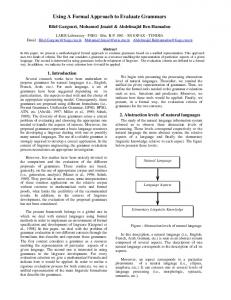
The cost function which controls the diagnosis generation process is simply the length of an incomplete diagnosis. An execution trace of the GEN-DIAG is shown in Figure 2, where (o), ( J )and ( x ) represent respectively the incomplete diagnoses, diagnoses and incomplete diagnoses that are subsumed by others, while [ A B ( . .] represents the conflict generated for the incomplete diagnosis.

Figure 2: The execution trace of the

GEN-DIAG

algorithm

First, the empty set was verified to be incoilsistent with S D U OBS and was initialized to be the only incomplete diagnosis. It was expanded by the conflict [ A B ( B ~.).,. ,AB(B,), A B ( C ~. ). ., ,AB(C,),AB(D)]. The incomplete diagnoses A B ( C ~.).,. ,AB(C,) and AB(D)were immediately checked out to be the single-fault diagnoses. Then the incomplete diagnosis A B ( B ~was ) expanded by the conflict [ A B ( A ~AB(B2), ), . . . ,AB(B,)]. Note that the singlefault diagnoses were used to reduce the size of the conflict. Except for ' A B ( B ~A) ,B ( A ~ which )' was checked out to be a diagnosis, every other element from the expansion was subsumed by an existing incomplete diagnosis and disca,rded. Other incomplete diagnoses are subsequently expanded in a similar fashion which produce additional diagnoses and incomplete diagnoses. One important observation from this example is that the space of incomplete diagnoses which the algorithm explores is much smaller than the entire set of possible incomplete . . . ,AB(B;,)where diagnoses. In particular, it only explores those of the form AB(B;,)? 1 5 il < . . . , < ik n instead of the much larger collection A B ( & ) , . . . ,AB(X;,) where X=AorX-B. In an experiment to see how a generate-and-test dia.gnostic system will perform, we modified the GEN-DIAG algorithm by expa.nding each incomplete diagnosis with the set of all assumptions except those useless ones as indicated in Propositions 10 and 11. A n empirical comparison was made between the G E N - D I A G a.lgorithlr1a.nd the genera,te-and-test algorithm