arXiv:cond-mat/9607077v1 11 Jul 1996 .... since Σv = 2(number of up spins) − 6 is a multiple of 3 iff the number of up spins itself is ..... y + y1/2(3x + 6x2 + x3)). 2.
arXiv:cond-mat/9607077v1 11 Jul 1996
T96/083
Folding of the Triangular Lattice with Quenched Random Bending Rigidity
P. Di Francesco, E. Guitter and S. Mori* Service de Physique Th´eorique, C.E.A. Saclay, F-91191 Gif sur Yvette Cedex, France
We study the problem of folding of the regular triangular lattice in the presence of a quenched random bending rigidity ±K and a magnetic field h (conjugate to the local
normal vectors to the triangles). The randomness in the bending energy can be understood
as arising from a prior marking of the lattice with quenched creases on which folds are favored. We consider three types of quenched randomness: (1) a “physical” randomness where the creases arise from some prior random folding; (2) a Mattis-like randomness where creases are domain walls of some quenched spin system; (3) an Edwards-Andersonlike randomness where the bending energy is ±K at random independently on each bond.
The corresponding (K, h) phase diagrams are determined in the hexagon approximation of the cluster variation method. Depending on the type of randomness, the system shows essentially different behaviors. 07/96 * Address after July 1996: Department of Physics, Graduate School of Science, University of Tokyo, Hongo 7-3-1, Bunkyo-ku, Tokyo 113, Japan
.
1. Introduction The statistical properties of polymerized membranes, or tethered surfaces have been widely discussed in the past few years [1-3].
A polymerized membrane is the two-
dimensional generalization of a linear polymer [1-4]. Its energy involves both an in-plane elastic (strain) contribution and an out-of-plane (bending) one. At low temperature, such a membrane with bending rigidity is asymptotically flat and its radius of gyration RG increases as the linear internal dimension L of the surface [5-10]. As a function of temperature, the membrane without self-avoiding interaction (phantom membrane) undergoes a crumpling transition from the low temperature flat phase to a high temperature crumpled √ phase (RG ∼ ln L) [11-12]. The mechanism of the transition, in particular the stability of
the flat phase, is rather subtle and relies on the coupling between in-plane and out-of-plane deformation modes [5].
Very generally, 2-dimensional membranes can be discretized into triangulations, whose faces are endowed with natural Heisenberg spin variables, representing the direction of the local normal vector to the surface [1]. Polymerized membranes, which have a fixed connectivity, then translate into statistical spin systems on the regular triangular lattice. The corresponding spin system is however involved, because the resulting spins are not independent variables. The constraint of being normal vectors to a surface causes a long range interaction between the spins, which stabilizes the ordered flat phase, as opposed to the case of the usual 2-dimensional unconstrained Heisenberg model, always disordered [1,5]. The above mechanism clearly indicates the subtlety of the correspondence between geometrical objects and spin systems, especially in two dimensions. In order to understand this, several simple models have been proposed. The simplest one is probably a square lattice model introduced by David and Guitter [7]. The model is a discrete rigid bond square lattice, which is allowed to fold onto itself along its bonds in a two-dimensional embedding space. The constraint there makes the folds propagate along straight lines. In the presence of bending rigidity, the system is always flat. A triangular lattice version of this 2D folding model was then introduced by Kantor and Jari´c [13]. Describing the (up or down) normal to each triangle by a spin variable σ = ±1, the model Hamiltonian translates into that of the Ising model with however 1
constrains on the spin variables. This results in several new features, and a totally new phase diagram, as compared with the usual Ising model [13-16]. Finally, the folding of the triangular lattice embedded in a 3-dimensional discrete space has been formulated as a 96-vertex model [17,18]. Constraints do not appear only in the physical degrees of freedom, like local normal vectors. If the membrane has disorder, the disorder itself can also be constrained in some cases. For example, if one folds a piece of paper and makes a crease, this will generate a spontaneous curvature along the crease. If one now crumples the paper randomly by hand [4,19], the generated spontaneous curvature will be directly related to the configuration of the normal vectors of the resulting crumpled configuration. For the latter to be accepted as a physical configuration, the normal vectors should also obey some constraints. The induced disorder (in this case the induced random spontaneous curvature) should thus obey similar “physical” constraints. Here we study a simple model of folding with such a “physical” quenched randomness. As a model, we use the triangular lattice with quenched random bending rigidity and clarify the importance of the “physical” constraints on the disorder. The paper is organized as follows. In section 2, we first discuss the general folding problem of the triangular lattice and recall some known facts about it. We then describe the precise type of randomness which we consider on the lattice and which we write as a Mattis-like spin system [20] with constraints. In section 3, we describe the cluster variation method that we shall apply to the study of the thermodynamics of the system [21-23]. We first describe the procedure for a general disordered system. We then restrict ourselves to the hexagonal approximation in which the clusters are made of a maximum of six triangles. Next, we analyze the pure (without disorder) system again, as a particular limiting case with trivial disorder. The results for the fully disordered system are presented in section 4. After giving a few results following from a reduced variable analysis, we present the complete phase diagram of the system. In section 5, we study other variants of the disorder. In particular, we discuss the specificity of the “physical” constraint on the random bending rigidity. We present for each type of disorder the corresponding phase diagram. Some concluding remarks are gathered in section 6.
2. Folding with Quenched Random Bending Rigidity In this section, we first recall the rules of folding for the triangular lattice [13]. We then introduce disorder in the problem in terms of a random bending rigidity. 2
2.1. Folding of the triangular lattice: pure case Let us consider a regular triangular lattice which can be folded onto itself along its bonds. We allow only for complete foldings which result in two-dimensional folded configurations. Each bond thus serves as a hinge between its two neighboring triangles and is in either one of the two states: folded (with the two neighboring triangles face to face) or not (with the two neighboring triangles side by side). A folded state of the system is entirely determined by the list of its folded bonds. In this definition, the folding process may cause self-intersections and the model corresponds to a “phantom” membrane. Also this does not distinguish between the different ways of folding which result in the same folded state.
(a)
(b)
(g)
(c)
(h)
(d)
(i)
(e)
(j)
(f)
(k)
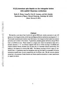
Fig. 1: The eleven local fold environments for a vertex. Folds are represented by thick lines. One of the two (opposite) possible spin configurations on the triangles is also indicated. One can easily see that, among the 26 possible fold configurations for the six bonds surrounding a given vertex, only 11 states are allowed, corresponding to actual foldings of the surrounding hexagon [13]. These configurations are displayed in fig 1. It can be checked that imposing everywhere one of these eleven local environments is sufficient to define the folding consistently throughout the lattice. The folding of the triangular lattice is thus simply expressed as an 11-vertex model on the lattice. Note that, even if the folding is defined locally, its nature is highly non-local. Since all vertices in Fig.1 have an even number of elementary folds, these folds form folding lines without endpoints. Moreover all “folded” vertices (vertices (b)-(k) in Fig.1) have at least one fold on the left half of the hexagon and one on the right. Thus folds are forced to propagate through the entire lattice [14]. Folding can also be expressed with spin variables σi = ±1 living on the elementary
triangles, which indicate whether the i-th triangle faces up or down in the folded state. The spin variable changes its sign between two neighboring triangles, if and only if their 3
common bond is folded, i.e. folding lines are domain walls of the spin system. One can think of the spin as the normal vector to the triangle. We depict the corresponding spin configurations on Fig.1. Note that there are two spin configurations for each folded state, due to the degeneracy under reversal of all spins. Clearly, the only allowed vertex environments are those with exactly 0, 3 or 6 surrounding up spins. In other words, for a spin configuration to correspond to a folded state, the six spins σi (i = 1, 2, · · · , 6) around any vertex v must satisfy the local constraint [14] Σv ≡
X
σi = 0 mod 3 ,
(2.1)
i around v
since Σv = 2(number of up spins) − 6 is a multiple of 3 iff the number of up spins itself is a multiple of 3. Folding is thus expressed here as a constrained Z2 spin system.
The statistical behavior of this system has been extensively studied, using a transfer matrix formalism [13,15], the correspondence with a solvable three-coloring model [14] and a cluster variation method [16]. Introducing a bending energy term −Jσi σj between
nearest neighbors and a magnetic field term −Hσi , the following model Hamiltonian was considered,
HIsing = −J
X
σi σj − H
(ij)
X
σi .
(2.2)
i
This is nothing but the Ising Hamiltonian, which is here however coupled to the local constraint (2.1). In the folding context, the magnetization simply measures the projected area of the lattice (i.e. the algebraic area of the domain enclosed by its boundary) and the magnetic field can thus be interpreted as a lateral tension term. For convenience we will use the reduced coupling and magnetic field K ≡ J/kB T ; h ≡ H/kB T .
(2.3)
The phase diagram of the system is shown in Fig.2. In order to characterize each phase, two order parameters are introduced. One is the usual magnetization, M=
X � 1 X h σi + σi i, Nt △
(2.4)
▽
and the other is the staggered magnetization Mst =
X � 1 X h σi − σi i, Nt △
4
▽
(2.5)
h
1.5
1.0
Compactly Ordered Folded Phase M=0 Mst >0
Completely Flat Phase M=+1 Mst =0
0.5
M=0 Mst =0 Kc K 0.2 0.4 0.6 Disordered Folded Phase -0.5 Completely Flat Phase M=-1 -1.0 Mst =0 -1.5
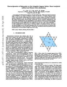
Fig. 2: Phase diagram in the (K, h) plane. Three first order lines h = hc (K), −hc (K) (K < Kc ) and h = 0 (K > Kc ) separate the three phases M = 0, ±1 and meet at the triple point (Kc , 0). The dashed line represents the transition line between the disordered folded phase M = 0, Mst = 0 and the compactly ordered folded phase M = 0, Mst 6= 0. where the sum is performed separately on triangles pointing up and down, dividing the original triangular lattice into two inter-penetrating sublattices. Here Nt is the total number of triangles in the system. Three phases exist: a completely flat phase (M = ±1, Mst = 0),
a disordered folded state (M = 0, Mst = 0) and a compactly ordered folded state (M = 0, Mst 6= 0) [15,16]. Note that the flat phase has a maximal magnetization |M | = 1
and is indeed frozen in the pure completely flat state with all spins aligned. There is no flat phase with intermediate (0 < |M | < 1) magnetization. Three first order transition
lines h = hc (K), −hc (K) (K < Kc ), and h = 0 (K > Kc ) separate the three phases
M = 0, ±1, with a triple point at Kc ∼ 0.1 (estimated from either the transfer matrix [15] or the cluster variation [16] approach). For negative K, the transition between the
disordered folded phase and a compactly ordered (antiferromagnetic) folded phase with staggered order parameter Mst 6= 0 is found to be continuous at h = 0 [16]. This transition
is represented by the broken line of Fig.2, which intersects the horizontal (h = 0) axis at K ∼ −0.284. We see here that, when compared with the usual unconstrained Ising model,
the phase diagram has been strongly modified. In particular, it is now asymmetric with respect to K with the usual continuous ferromagnetic transition replaced by an abrupt first order transition to a completely ordered phase. 5
2.2. Quenched random bending rigidity What kind of disorder should one introduce in the above model (Eq.(2.2))? Since we are dealing with folding of a phantom object with a two-dimensional resulting folded state, we cannot distinguish between ±180 degree folds, thus we cannot introduce any
spontaneous curvature term. Disorder will appear here in the form of a random bending rigidity Kij . The most general Hamiltonian with random nearest neighbor coupling Kij
and a constant external field h is (we drop the kB T factor, thus using reduced coupling constants) Hrandom =
X (ij)
−Kij σi σj − h
X
σi .
(2.6)
i
There are several possible choices for Kij . One possibility is the Edwards-Anderson model for spin-glasses [24], where Kij = ±K independently on each bond. Such a model is
interesting as it may have a spin glass phase. In such a phase, spins are randomly oriented (M = 0 and Mst = 0), but the following order parameter q takes a nonzero value 1 X q= hσi i2 . Nt i
(2.7)
Here the upper bar stands for the quenched average over the randomness. We shall discuss this type of disorder in section 5. As has been discussed in the introduction, we are interested in another type of “physical” disorder where the random bending rigidity has been generated by a prior irreversible folding of the lattice [4,19]. We have in mind the picture of a crumpled piece of paper marked with irreversible creases. The effect of this irreversible crumpling is to impose the corresponding crumpled state as the new ground state of the system. No frustration will occur as long as one does not strain the paper. The model Hamiltonian should thus have that crumpled state as its ground state and this information should be included in Kij . One natural choice for Kij with a “random” ordered phase and no frustration is that of a Mattis Model [20]. In this model, the bending rigidities Kij are functions of a set of random face variables τi : Kij = Kτi τj .
(2.8)
The τi = ±1 are “frozen” according to a specified probability distribution ρτ (τ1 , τ2 · · · , τNt )
reminiscent of the first irreversible crumpling process. The total Hamiltonian is then given by HMattis = −K
X (ij)
τ i τ j σi σj − h 6
X i
σi .
(2.9)
As is well-known, if there is no constraint on spin variables, the following gauge transformation σi′ → σi τi
(2.10)
makes the above model (2.9) in zero external field h = 0 equivalent to the pure system [20]. At K = ∞, the state with σi = τi is recovered as the ground state.
In our model, the spin variables are constrained by Eq.(2.1) and the above gauge trans-
formation cannot be performed since it does not preserve the folding constraint. Moreover, the ground state σi = τi can be reached only if the τ variables themselves obey the folding constraint: X
τi = 0 mod 3 .
(2.11)
i around v
This type of τ -configuration is what we call a “physical” disorder. We shall restrict ourselves to this type of disorder in the following sections 3 and 4. We will return to other types of disorder (such as the Edwards-Anderson model) later in section 5. From the above discussion, we understand the physical origin of the local constraint on the τ -variables. Then what probability distribution ρτ (τ1 , τ2 · · · , τNt ) should we use for
them? Since the τ variables obey the same constraint as the pure σ system described in
the first part of this section, we can take advantage of the solution of this pure system by simply assuming that the τ distribution is described by a particular (appropriately chosen) point in the disordered phase of the phase diagram of Fig.2. A natural choice is the point at the origin of the phase diagram (K = h = 0) since it then does not involve any energy parameter for the disorder and treats as equiprobable all allowed configurations of “physical” disorder. In other words, we shall take for the distribution ρτ (τ1 , τ2 · · · , τNt )
the density of the pure constrained problem at K = h = 0. Due to the constraint, this density remains non-trivial.
3. Cluster Variation Method for the Disordered System In this section we explain in detail the hexagon approximation of the cluster variation method (CVM) generalized to a random system [21-23]. In subsection 3.1, we explain the method in the general case. In subsection 3.2, we apply the CVM to the pure system (Kij = K) as a limiting case with trivial disorder. As mentioned above, this is also instrumental to give an explicit form for ρτ which is necessary to tackle the fully disordered case. We also discuss several symmetry breakings of the model. 7
3.1. The CVM and its hexagon approximation The CVM is a closed-form approximation based on the minimization of an approximated free energy density functional, which is obtained by a truncation of the cluster expansion of the full free energy density functional appearing in the exact variational formulation of the problem [25,26]. Consider our spin system σi with Nt sites and Hamiltonian (2.6)[23]. The configuration of the random bond couplings Kij is specified by a probability distribution P ({Kij }). In our case of “physical” disorder where Kij = Kτi τj , we shall have: P ({Kij = Kτi τj }) = ρτ (τ1 , · · · , τNt ).
(3.1)
The discussion below is however more general. In terms of a density matrix ρ(σ1 , σ2 , · · · , σNt |{Kij }) for each configuration {Kij },
we define the variational free energy associated with the Hamiltonian Hrandom (σ, {Kij })
(from now on, we use the notation σ = {σi }) as hX i F ({Kij }) = ρ(σ|{Kij })[Hrandom (σ, {Kij }) + ln ρ(σ|{Kij })]
min
σ
.
(3.2)
The subscript min means that the above expression must be taken at its minimum with respect to ρ(σ|{Kij }). This is the well-known variational principle. The minimization is performed at fixed {Kij } with the normalization constraint: X σ
ρ(σ|{Kij }) = 1.
(3.3)
The quenched free energy F is then given by F=
X
{Kij }
P ({Kij })F ({Kij }),
(3.4)
where the sum extends over all possible realizations of the disorder. Upon introducing the generalized density matrix ρ(σ, {Kij }) = P ({Kij })ρ(σ|{Kij }),
(3.5)
one can easily show that h X i F= ρ(σ, {Kij })[Hrandom (σ, {Kij }) + ln ρ(σ, {Kij })]
min
σ,{Kij }
8
+ SDis
(3.6)
where the minimization is now on a density ρ(σ, {Kij }) for both σ and {Kij } with the constraint X σ
ρ(σ, {Kij }) = P ({Kij }).
(3.7)
The quantity SDis is a constant term depending only on the probablity distribution for the disorder and reads SDis = −
X
{Kij }
P ({Kij }) ln P ({Kij }).
(3.8)
of the expectation value
In such a scheme it can be shown that the quenched average < A(σ, {Kij }) > of an operator A(σ, {Kij }) is given by < A(σ, {Kij }) > = =
X
{Kij }
X
P ({Kij }) < A(σ, {Kij }) > (3.9)
{Kij },σ
ρmin (σ, {Kij })A(σ, {Kij }).
where ρmin (σ, {Kij }) is the density at the minimum of the quenched free energy functional (3.6). The CVM is obtained by taking the thermodynamic limit Nt → ∞ and truncating the P cumulant expansion for the entropy S ≡ − σ,{Kij } ρ(σ, {Kij }) ln ρ(σ, {Kij }) appearing in (3.6) to a set of “maximal preserved clusters” Γi , i = 1, 2, · · · , r (and all their translated images). The variational principle will then be applied to the reduced density matrix ρΓi (σ, {Kij }) associated with the maximal preserved clusters Γi , i.e. the minimization will be performed on this reduced set of densities.
1 2
6 3
1 2
5 4
A B
Fig. 3: Labeling of the spins on an elementary hexagon. Each site i (= 1, · · · , 6) supports a spin variable σi and a disorder variable τi . The reduction process from ρ6 to ρ2 and to ρ1A(B) is also indicated. 9
In the hexagon approximation for the triangular lattice, the largest clusters appearing in the expansion are hexagons. Hereafter we restrict our presentation to the case of the Mattis like coupling Kij = Kτi τj . For the other cases, the generalization is straightforward. We introduce the reduced density matrix for a hexagon. ρ6 (σ1 , σ2 , σ3 , σ4 , σ5 , σ6 , τ1 , τ2 , τ3 , τ4 , τ5 , τ6 ).
(3.10)
The spins in the argument of ρ6 follow each other counterclockwise in the hexagon, and the first one is on the A sublattice (see Fig.3) i.e. is pointing up. This reduced density matrix represents the probability for one hexagon to have fixed values of σ and τ . It is normalized according to X {σ}
ρ6 ({σ}, {τ }) = ρτ,6 ({τ }),
(3.11)
where ρτ,6 is the 6-point probability for the disorder variable on a hexagon as obtained from the corresponding partial trace of ρτ (τ1 , · · · , τNt ) in the thermodynamic limit. We assume
that this 6-point reduced density is the same for each hexagon, i.e. that the distribution of disorder is translationaly invariant. We also introduce the site and pair density matrices ρ1A(B) (σ1 , τ1 ), ρ2 (σ1 , σ2 , τ1 , τ2 ), which are defined as symmetrized partial traces of ρ6 by ρ2 (σ1 , σ2 , τ1 , τ2 ) ≡
1 6
X
[ρ6 (σ1 , σ2 , σ3 , σ4 , σ5 , σ6 , τ1 , τ2 , τ3 , τ4 , τ5 , τ6 )
σ3 ,σ4 ,σ5 ,σ6 τ3 ,τ4 ,τ5 ,τ6
+ ρ6 (σ3 , σ2 , σ1 , σ4 , σ5 , σ6 , τ3 , τ2 , τ1 , τ4 , τ5 , τ6 ) + ρ6 (σ3 , σ4 , σ1 , σ2 , σ5 , σ6 , τ3 , τ4 , τ1 , τ2 , τ5 , τ6 ) + ρ6 (σ3 , σ4 , σ5 , σ2 , σ1 , σ6 , τ3 , τ4 , τ5 , τ2 , τ1 , τ6 ) + ρ6 (σ3 , σ4 , σ5 , σ6 , σ1 , σ2 , τ3 , τ4 , τ5 , τ6 , τ1 , τ2 )
(3.12)
+ ρ6 (σ1 , σ3 , σ4 , σ5 , σ6 , σ2 , τ1 , τ3 , τ4 , τ5 , τ6 , τ2 )], ρ1A (σ1 , τ1 ) ≡ ρ1B (σ2 , τ2 ) ≡
X
ρ2 (σ1 , σ2 , τ1 , τ2 ),
X
ρ2 (σ1 , σ2 , τ1 , τ2 ).
σ2 ,τ2
σ1 ,τ1
Here we have introduced two site density matrices, ρ1A and ρ1B , corresponding to the two inter-penetrating sublattices in which the triangular lattice can be divided (see Fig.3). 10
After the appropriate truncation of the cumulant expansion of S at the level of hexago-
nal clusters, we get the approximate CVM quenched free energy per hexagon as a functional of ρ6 ({σi }, {τi }) only (by implicit use of Eq.(3.12))[25], f (ρ6 ({σi }, {τi})) = −3KTrσ,τ (τ1 τ2 σ1 σ2 ρ2 (σl , σ2 , τ1 , τ2 )) − hTrσ (σ1 ρ1A (σ1 , τ1 ) − hTrσ (σ2 ρ1B (σ2 , τ2 ) + Trσ,τ (ρ6 ln ρ6 ) − 3Trσ,τ (ρ2 ln ρ2 ) + Trσ,τ (ρ1A ln ρ1A ) + Trσ,τ (ρ1B ln ρ1B ) h i + Trτ λτ ({τi })(Trσ ρ6 ({σi }, {τi }) − ρτ,6 ({τi }))
(3.13)
+ Sτ , to be minimized with respect to ρ6 ({σi }, {τi })1 . Here Tr stands for trace and λτ ({τi })
are Lagrange multipliers which ensure the normalization of ρ6 ({σi }, {τi}), according to
Eq.(3.11). Sτ is the entropy for the disorder variable τi , for which we also use the CVM estimate: Sτ = Trτ (ρτ,6 ln ρτ,6 ) − 3Trτ (ρτ,2 ln ρτ,2 ) + 2Trτ (ρτ,1 ln ρτ,1 ),
(3.14)
where ρτ,2 and ρτ,1 are partial (symmetrized) traces of ρτ,6 . With the above definitions, our free energy can be regarded as a function of ρ6 only and taking the derivative with respect to a generic element of ρ6 we find the stationarity conditions ρ6 ({σi }, {τi }) = exp[−λτ ({τi }) +
K X h X τi τi+1 σi σi+1 + σi ] 2 i=1,6 3 i=1,6
× [ρ2 (σ1 , σ6 , τ1 , τ6 )ρ2 (σ1 , σ2 , τ1 , τ2 )ρ2 (σ3 , σ2 , τ3 , τ2 ) ρ2 (σ3 , σ4 , τ3 , τ4 )ρ2 (σ5 , σ4 , τ5 , τ4 )ρ2 (σ5 , σ6 , τ5 , τ6 )]
(3.15)
1/2
× [ρ1A (σ1 )ρ1B (σ2 )ρ1A (σ3 )ρ1B (σ4 )ρ1A (σ5 )ρ1B (σ6 )]−1/3 , with the convention σ7 = σ1 , τ7 = τ1 . 1
The cumulant expansion of the entropy can be understood as follows. We write the truncated
entropy as S=
X
hexagons H
SH −
X
pairs P
SP +
X
ST
triangles T
where we must first subtract the contribution of pairs of neighboring triangles and re-add that of single triangles to avoid overcounting. Noting that the numbers NH , NP , NT A and NT B of respectively hexagons, pairs and triangles of the sublattices A and B satisfy NP /NH = 3, NT A /NH = NT B /NH = 1, this leads to the entropy per hexagon appearing in (3.13).
11
One can solve this set of equations with the definitions of Eqs.(3.12) and the normalization constraint (3.11) by the so-called natural iteration method [21]. Starting from some assumption on ρ2 and iterating the above equation, ρ6 converges to a solution of (3.15) which is moreover a local minimum of the approximate free energy (3.13). To find a global minimum, it is in general necessary to start the iteration with different sets of initial conditions on ρ2 appropriately chosen to reach the different expected phases. At each step, the normalization condition (3.11) is recovered by adjusting the Lagrange multiplier for each realization of the disorder on the hexagon. Before going to the analysis of the model with disorder, in the next subsection we will revisit the pure case [16]. One reason is that we need to fix the probability distribution for the disorder variables ρτ ({τi }). 3.2. Pure case and explicit form for ρτ In this section, we reconsider the pure case for h = 0 in detail within the CVM approximation as a particular trivial realization of disorder where all Kij are constant and equal to K [16]. We only need to consider the “pure” 6-point functions ρ6 (σi ), which does not depend on the τi variable any longer. We can easily recognize that the 2 × 11 =
22 elements of ρ6 , which correspond to the weights for each state in Fig.1, are not all independent since some of the states are related by simple symmetries and should thus have the same weight. This of course assumes that the corresponding symmetries are not spontaneously broken. Hereafter we only consider the system for h = 0 and consider three types of solutions corresponding to the three different symmetries of the spin system in the phase diagram of Fig.2 [16]: (1) Disordered folded phase: we do not allow for any spontaneous symmetry breaking in the system. Using rotational symmetry and the symmetry under reversal of all spins, we end up with only 4 independent weights Z0,1,2,3 corresponding to vertices with respectively 0,2,4 or 6 surrounding folds. (2) Ferromagnetic phase: we allow for a spontaneous ferromagnetic symmetry breaking (M 6= 0). Then the two vertices with no fold have different weight Z0 and Z0 according
to their ±6 magnetization. The other vertices are neutral in this respect and we end up with 5 different weights.
(3) Antiferromagnetic phase: we allow for a spontaneous antiferromagnetic symmetry breaking (Mst 6= 0). Then all weights Zi have to be doubled into (Zi , Zi ) except for
the vertex with no fold (i = 0) which is neutral in the staggered magnetization. We
end up with 7 different weights. 12
Spin Conf.
(1) Dis.
(2) Ferro.
(3) A.Ferro.
Deg.
+ + + + ++
Z0
Z0
Z0
1
− − − − −−
Z0
Z0
Z0
1
+ + + − −−
Z1
Z1
Z1
3
− − − + ++
Z1
Z1
Z1
3
+ − − + +−
Z2
Z2
Z2
6
− + + − −+
Z2
Z2
Z2
6
+ − + − +−
Z3
Z3
Z3
1
− + − + −+
Z3
Z3
Z3
1
Table I: Independent hexagon spin configurations. The corresponding elements of ρ6 and the degeneracies are indicated.
The spin configurations, their degeneracies and the notations for their weights are summarized in Table I. Of course, the case (1) can be recovered from either case (2) or (3) as a particular realization with no spontaneous symmetry breaking (i.e Zi = Zi for all i). Also, we assume that the two (ferromagnetic and antiferromagnetic) symmetries cannot be broken simultaneously. We thus need to study only the cases (2) and (3) above to get the complete phase diagram of the system (here at h = 0). At first we consider the ferromagnetic case (2). In this case, the stationarity condition reduces to the following nonlinear equations between the weights Z0 , Z0 , Z1 , Z2 , Z3 . Z0 = exp(−λ + 3K)(y++ )3 /(y+ )2 Z0 = exp(−λ + 3K)(y−− )3 /(y− )2 Z1 = exp(−λ + K)(y++ )(y−− )(y+− )/(y+ )(y− )
(3.16)
Z2 = exp(−λ − K)(y++ )1/2 (y−− )1/2 (y+− )2 /(y+ )(y− ) Z3 = exp(−λ − 3K)(y+− )3 /(y+ )(y− ), involving a single Lagrange multiplier λ. Here, y++ , y+− , y−− , y+ and y− are two- and one-point functions ρ2 (σ1 σ2 ) and ρ1 (σ1 ) (there is no difference here between sublattices A 13
and B), which are defined as follows, y++ = ρ2 (++) = Z0 + 2Z1 + 2Z2 y+− = ρ2 (+−) = ρ2 (−+) = Z1 + 4Z2 + Z3 (3.17)
y−− = ρ2 (−−) = Z0 + 2Z1 + 2Z2 y+ = ρ1 (+) = Z0 + 3Z1 + 6Z2 + Z3 y− = ρ1 (−) = Z0 + 3Z1 + 6Z2 + Z3 . The above equations imply the following simple relations: (Z0 Z0 )1/2 Z1 Z2 (y++ )1/2 (y−− )1/2 = = = exp(2K) . Z1 Z2 Z3 y+−
(3.18)
Introducing the two reduced variables x≡
Z1 , (Z0 Z0 )1/2
y≡
Z0 . Z0
(3.19)
we can express all the weights in terms of x, y and the normalization factor w0 ≡ (Z0 Z0 )1/2 . Z0 = y +1/2 w0 , Z1 = xw0 ,
Z0 = y −1/2 w0 Z2 = x2 w0 ,
Z3 = x3 w0 .
(3.20)
The above equations (3.16) reduce to the following nonlinear equations for the reduced variables, y=
x=
y + 2y 1/2 (x + x2 ) �3 1 + y 1/2 (3x + 6x2 + x3 ) �2 . 1 + 2y 1/2 (x + x2 ) y + y 1/2 (3x + 6x2 + x3 )
(3.21)
y(x + 4x2 + x3 ) . u(1 + 2y 1/2 (x + x2 ))1/2 (y + 2y 1/2 (x + x2 ))1/2
(3.22)
where u = exp(2K). The parameter y measures the spontaneous ferromagnetic symmetry breaking while the parameter x measures the fugacity per folded bond. We can easily see that Eq.(3.21) has two obvious solutions: a solution y = 1 and x arbitrary and a solution x = 0 and y arbitrary. The latter solution is also a solution of Eq.(3.22). It means that each vertex of the membrane can be only in one of the two configurations without fold Z0 or Z0 . The solution cannot determine the ratio y = Z 0 /Z0 , i.e the proportion of each state. However, with only these two vertices at hand, no fold can be ever created and the only possible global states for the lattice are the state with 14
all spins up (M = 1) and that with all spins down (M = −1). The above solution simply
describes an arbitrary superposition of these two (symmetric) pure flat states. The fact that the membrane is indeed frozen in a pure completely flat state is further confirmed by computing the entropy which is found to be exactly zero, and by computing the free energy, which is found to be f = −3K per hexagon, as expected (there are 3 bonds per hexagon).
The first solution with y = 1 means that the spontaneous symmetry breaking does not occur and that the membrane is in the disordered folded state (Z0 = Z0 ). The value of x is then fixed by Eq.(3.22)[16]: p (2 − u) + (3 − u − u2 ) x= (2u − 1)
(3.23)
√ which has a solution for K ≤ ln((1 + 13)/2)/2. Comparing the corresponding free energy
to that of the pure flat state, we get a first order transition from disordered folded to purely flat at Kc ∼ 0.1013 [16].
We also looked numerically for another non-trivial solution with spontaneous symme-
try breaking (y 6= 1) and intermediate magnetization (x 6= 0) but did not find any. We
conclude that there is no possible flat phase with 0 < |M | < 1 and the above three phases (M = ±1 or 0) are the only stable ones for positive K.
P0 2
P1 6
P2 12
P3 2
Fig. 4: Probability distribution for each disorder configuration. We also show their degeneracies As has been discussed previously, the above analysis is also instrumental for the estimation of the probability distribution ρτ,6 ({τi }) of the disorder variables τ . We can use
indeed for ρτ,6 the distribution ρ6 above at K = h = 0, characterized by y = 1 and x = 2 [16]. In other words, if we define P0,1,2,3 as the weights ρτ,6 for the local realiza-
tions of disorder with 0,2,4 or 6 creases around the vertex, we learn that the ratios P1 /P0 , 15
P2 /P1 and P3 /P2 must all be identical and equal to 2. Their values are then fixed by the normalization: 2P0 + 6P1 + 12P2 + 2P3 = 1
(3.24)
leading to [16]:
2 4 8 1 , P1 = , P2 = , P3 = . (3.25) 78 78 78 78 More generally, we can parametrize the distribution of P with one parameter α equal P0 =
to the ratios α = P1 /P0 = P2 /P1 = P3 /P2 . Beside the natural value α = 2 above, the limiting case α = 0 describes a membrane with no crease and Kij = K everywhere, while α = ∞ describes a membrane with creases everywhere and Kij = −K on each bond. Now we discuss the compactly ordered (antiferromagnetic) folded phase (3). There are 7 independent weights for h = 0 (see Table I) and in this case it is convenient to use staggered variables ηi = (−1)i−1 σi with (−1)i−1 = 1 on triangles belonging to the sublattice A and (−1)i−1 = −1 on triangles belonging to the sublatice B. The corresponding
two-point function is simply
ρη,2 (η1 , η2 ) = ρ2 (η1 , −η2 ).
(3.26)
About the one-point function, we have the symmetry ρ1A (σ) = ρ1B (−σ) in the antiferromagnetic phase, leading to only one (A/B independent) one-point function for η: ρη,1 (η) = ρ1A (η) = ρ1B (−η)
(3.27)
As before, the solution of the non-linear stationarity equations for the 7 weights can be parametrized as: Z0 = w0 ,
Z1 = xy 1/2 w0 ,
Z1 = xy −1/2 w0
Z2 = x2 y 1/2 w0 , Z2 = x2 y −1/2 w0 Z3 = x3 y 3/2 w0 , Z3 = x3 y −3/2 w0 .
(3.28)
with two reduced variables x and y solutions of, y++ y− �2/3 y= , y−− y+
x=u
1/2 1/2 −1 y++ y−−
y+−
.
(3.29)
where y++ = ρη,2 (++) = Z1 + 3Z2 + Z2 + Z3 y+− = ρη,2 (+−) = ρη2 (−+) = Z0 + Z1 + Z1 + Z2 + Z2 y−− = ρη,2 (−−) = Z1 + 3Z2 + Z2 + Z3 y+ = ρη,1 (+) = Z0 + 2Z1 + Z1 + 4Z2 + 2Z2 + Z3 y− = ρη,1 (−) = Z0 + 2Z1 + Z1 + 4Z2 + 2Z2 + Z3 . 16
(3.30)
In the equations (3.29), the global normalization w0 drops out, so the equations can be solved for x and y as functions of u = exp(2K). Again the variable x measures the fugacity for each fold and y measures the antiferromagnetic spontaneous symmetry breaking. Solving the above equations numerically by iteration, we find a continuous transition from a disordered folded state (y = 1) to a compactly folded ordered phase (y 6= 1) at
Kst = −0.2838. The value of Kst can be found simply by linearizing the equations (3.29) by writing y = 1 + ǫ. This fixes the value of x to be the real solution xst of
that is
x3 − 21x2 − 12x − 4 = 0
(3.31)
√ √ xst = 7 + (387 + 2 223)1/3 + 53/(387 + 2 223)1/3
(3.32)
and u to be ust =
1 + 4xst + x2st . 1 + 2xst + 2x2st
(3.33)
4. Results for the fully disordered system In this section we analyze the fully disordered case (Eq.(2.9)) within the CVM approximation. In subsection 4.1, we study the system for h = 0 for several values of the parameter α for the disorder weights. Next we fix α = 2 and proceed to the general (K, h) case in subsection 4.2. We obtain the (K, h)-phase diagram by use of the natural iteration method. 4.1. Analysis with reduced elements of ρ6 (h = 0 case)
As in the previous section, we will study the fully disordered system for h = 0 by reducing the number of elements of the 6-point density matrix. In the case with disorder, the symmetries of the elements of the 6-point function ρ6 ({σi }, {τi }) de-
pend also on the symmetry of the disorder (τ -variables), in addition to the symmetries of
the spin variable {σ} itself.
In the previous section, we have studied the pure model with an antiferromagnetic
spontaneous symmetry breaking for K < 0. There we have used the staggered variables as ηi = (−1)i−1 σi . If we regard the pure system for K < 0 as a trivial disordered system with 17
τ config.
ηconfig.
+
Z +0,0 1
τ config.
-
ηconfig.
Z 0,0 1
Z 3,0 2
Z 0,1 3x2
+
Z 0,2 6x2
+
Z 0,3 2
-
+
+
Z 3,3 1
+
- Z -3,1 3 - + Z 3,2 6 - Z -3,3 1
+ Z 3,1 3
+ - Z3,2 6
Z 1,0 2 τ config.
+
+
Z 2,0 2 τ config.
Z +1,1 - Z -1,1 1 1 - + ~+ - ~+ - + Z 1,1 + - Z 1,1 2 2 + + - Z 1,2 - + Z 1,2 2 2 + ~ ~ + + - + Z 1,2 + - Z 1,2 4 4 + + + + Z 1,3 - - Z 1,3 + - 1 1 +
ηconfig.
- Z +2,1 - + 1 ~+ + - + - Z 2,1 + - + 2 + + Z 2,2 1 - _+ + + + Z 2,2 - + - 1 ~+ + - + Z 2,2 + - 2 -+ + Z +2,2 + 2 - + Z +2,3 + 1 +
Z 2,1 1 ~Z 2,1 2 Z 2,2 1 _Z 2,2 1 ~Z 2,2
2 Z 2,2 2 Z2,3
1
ηconfig.
Fig. 5: The 38 independent local fold environments for each vertex for the 4 different local realizations of disorder (0,2,4,or 6 creases). Each disorder configuration is shown at the left hand side of each group. To their right, we show the spin configurations, the weights and the degeneracies. We have represented by thick lines the domain walls for the gauged spin variable ηi = σi τi . A subscript i, j indicates a configuration with 2i creases and 2j folds. The superscript ± indicates a ± contribution to F . In a F = 0 phase, equating the + and − weights leaves us with 22 independent weights. ρτ,6 (1, −1, 1, −1, 1, −1) = 1, i.e. τi is fixed to (−1)i−1 , and K > 0, the above staggered variables can be written as
ηi = σi τi .
(4.1)
The motivation for introducing the staggered variables is that in these variables the antiferromagnetic order parameter Mst is simply written as 1 X � ηi i, Mst = h Nt i 18
(4.2)
and we don’t have to differentiate between the A- and B-sublattices. That is, the staggered variables {ηi } are more natural than the original variables {σi } when one discusses the
antiferromagnetic symmetric case.
In the fully disordered system, we are mainly interested in the spontaneous symmetry breaking at K > 0 of the following “frozen” order parameter2 F =
� 1 X h σi τi i. Nt i
(4.3)
This order parameter judges whether or not the membrane is trapped in the randomly oriented phase, characterized by the disorder variables {τi }. As in the antiferromagnetic case, it is natural to use the following “gauged” variables, ηi = σi τi .
(4.4)
Using these new gauged variables, we classify the elements of 6-point functions by the symmetries of both the spin configuration and the disorder configuration. Hereafter we only consider the system for h = 0 and allow for two types of solutions which correspond to whether the frozen order exists (F 6= 0) or not (F = 0).
(1) Disordered folded phase: we do not allow for any spontaneous symmetry breaking in the system (M, Mst and F = 0). Each of the 4 elementary types of disorder configuration (with 0,2,4 or 6 creases) leaves us with a certain number of symmetries, including that under reversal of all spins. We use these symmetries on the η variables to reduce the number of weights. We end up with only 22 independent weights in this case.
(2) Frozen phase: we allow for a spontaneous symmetry breaking of the frozen order parameter (F 6= 0). Then all weights have to be doubled except for those vertices P6 which are neutral in the gauged magnetization ( 1 ηi = 0). We end up with 38 different weights in this case.
In Fig.5, we have summarized the results of this symmetry analysis in the case (2). Note that case (1) can always be seen as a particular case of case (2) with extra symmetries. On the left hand side of each group, we show the disorder configuration {τi }. To its right, 2
The reader might wonder whether the τ → −τ symmetry could lead to a zero quenched av-
erage of the order parameter. However, this symmetry implies only that whenever ρmin ({σ}, {τ }) is a solution of the variational equations, ρmin ({σ}, {−τ }) is also a solution, but does not imply that ρmin ({σ}, {τ }) = ρmin ({σ}, {−τ }).
19
+
-
+ y0,0
y0,0
y0,1
+
-
y1,1+
y1,1
y1,0 τ config.
η config.
Fig. 6: Definitions of two-point functions. Gauged spin variables ηi = σi τi are used. On the left hand side, we show the disorder configuration τ . we present the spin configurations {ηi } which are independent from each other. We also indicate the notations for their weights and their degeneracies. The two indices i, j in Zi,j
indicate a configuration with 2i creases and 2j folds in the σ variable. In terms of these elements of the 6 point function, we define the two-point functions as follows, ± ± ± ± ± y0,0 = Z0,0 + 2Z0,1 + 2Z0,2 + 2Z1,0 + 2Z1,1 + 2Z˜1,1 + 2Z1,2 ± ± ± ± ± + 2Z˜1,2 + 2Z2,0 + 2Z2,1 + 2Z˜2,1 + 2Z2,2 + 2Zˆ2,2 , + − + − y0,1 = Z0,1 + 4Z0,2 + Z0,3 + Z˜1,1 + Z˜1,1 + Z1,2 + Z1,2 + − + − + + 3Z˜1,2 + 3Z˜1,2 + Z1,3 + Z1,3 + Z˜2,1 + − + + − + 2Z˜2,2 + Z˜2,1 + Z 2,2 + Z 2,2 + 2Z˜2,2 + − + − + Zˆ2,2 + Zˆ2,2 + Z2,3 + Z2,3 ,
(4.5)
y1,0 = y0,1 (Zi,j → Zj,i ),
± ± ± ∓ ± ± ± ∓ y1,1 = Z1,1 + Z1,2 + Z1,2 + 2Z˜1,2 + Z1,3 + Z2,1 + Z2,1 ± ± ± ∓ ± + 4Z2,2 + 2Z 2,2 + 4Zˆ2,2 + 2Zˆ2,2 + 4Z˜2,2 ± ∓ ± ± ± + 3Z2,3 + Z2,3 + 2Z˜2,1 + Z3,3 + 3Z3,2 ∓ ± + Z3,2 + Z3,1 .
The upper right index of y means that the gauged spin configuration {ηi } have the cor-
responding positive (or negative) contribution to F . Again, the first lower right index indicate whether there is a crease line (1) or not (0). The second index means that there 20
is a fold (1) or not (0) in the original σ variables. Based on these two-point functions, we also introduce the following one point functions, ± ± y ± = y0,0 + y0,1 + y1,0 + y1,1 .
(4.6)
In terms of these functions, we write down the stationarity conditions. For example, ± let us show those for Z0,0 , Z0,1 , Z0,2 and Z0,3 . + + 3 Z0,0 = exp(−λ0 + 3K)(y0,0 ) /(y + )2 , − − 3 Z0,0 = exp(−λ0 + 3K)(y0,0 ) /(y − )2 , + − Z0,1 = exp(−λ0 + K)(y0,0 )(y0,0 )(y0,1 )/(y + )(y − ),
(4.7)
+ 1/2 − 1/2 Z0,2 = exp(−λ0 − K)(y0,0 ) (y0,0 ) (y0,1 )2 /(y + )(y − ),
Z0,3 = exp(−λ0 − 3K)(y0,1 )3 /(y + )(y − ). Here, due to the above symmetries, we need only 4 Lagrange multipliers λ0,1,2,3 , one for each of the 4 elementary types of disorder in Fig.4. These Lagrange multipliers are of course determined by the normalization conditions, like + − Z0,0 + Z0,0 + 6Z0,1 + 12Z0,2 + 2Z0,3 = P0 .
(4.8)
As in the pure case, we introduce reduced variables. Here we need 4 ratios x, y, s and t defined as, x = u−1
y0,1 + − 1/2 , (y0,0 y0,0 )
y = u−1
+ �1/2 y− �1/3 y0,0 s= − , y+ y0,0
t=
y1,0 + − 1/2 , (y1,1 y1,1 ) + �1/2 y− �1/3 y1,1 , − y+ y1,1
(4.9)
and for convenience, we also introduce the following averaged weights, + − 1/2 w0 = (Z0,0 Z0,0 ) ,
+ − 1/2 w1 = (Z1,1 Z1,1 ) ,
+ − 1/2 w2 = (Z2,2 Z2,2 ) ,
+ − 1/2 w3 = (Z3,3 Z3,3 ) .
(4.10)
The stationarity conditions are then reduced to the following simple form, ± Z0,0 = s±3 w0 ,
Z0,1 = xw0 ,
Z3,0 = y 3 w3 ,
± Z3,1 = y 2 t±1 w3 ,
Z0,2 = x2 w0 , ± Z3,2 = yt±1 w3 ,
± Z1,1 = s2 t±1 w1 ,
± Z1,2 = xs±1 w1 ,
± Z˜1,2 = x3/2 y 1/2 (st)±1/2 w1 ,
± Z˜2,2 = xyt±1 w2 ,
(4.11)
± Z2,1 = ys±1 w2 ,
Z2,0 = y 2 w2 ,
± Z˜2,1 = x1/2 y 3/2 (st)±1/2 w2 ,
± Z3,3 = t±3 w3 ,
± Z˜1,1 = xys±1 w1 ,
Z1,0 = yw1 ,
± Z1,3 = x2 t±1 w1 ,
Z0,3 = x3 w0 ,
± Z2,2 = s±1 t±2 w2 ,
± Zˆ2,2 = x1/2 y 1/2 (st)±1/2 w2 ,
21
±
Z 2,2 = xyt±1 w2 , ± Z2,3 = xt±1 w2 .
Each weight Zi,j is given as the product of wi by a simple function of x, y, s and t. The rules for the x and y variables are simple: The disorder configuration splits the bonds into those which support a crease and those which do not. On the bonds with no crease, we √ assign a factor x if the bonds has a fold and 1 otherwise. On the bonds with a crease, we √ assign a factor y if the bond has no fold and 1 otherwise. In both cases, the non trivial factor is assigned if the gauged variable changes sign when crossing the bond. About the factors of s and t, the rules are more subtle. Still s and t both measure the symmetry breaking of the frozen parameter. The weights w0,1,2,3 can be expressed as functions of x, y, s and t thanks to the normalization conditions as follows, P0 = w0 [s3 + s−3 + 6x + 12x2 + 2x3 ], P1 = w1 [2y + s2 t + s−2 t + 2xyz + 2xyz −1 + 2xy + 2xy −1 + 4x3/2 y 1/2 s1/2 t1/2 + 4x3/2 y 1/2 s−1/2 t−1/2 + x2 t + x2 t−1 ], P2 = w2 [2y 2 + ys + ys−1 + 2x1/2 y 3/2 s1/2 t1/2 + 2x1/2 y 3/2 s−1/2 t−1/2
(4.12)
+ st2 + s−1 t−2 + 3xyt + 3xyt−1 + 2x1/2 y 1/2 s1/2 t1/2 + 2x1/2 y 1/2 s−1/2 t−1/2 + xt + xt−1 ] P3 = w3 [t3 + t−3 + 6y(t + t−1 ) + 3y 2 (t + t−1 ) + 2y 3 ]. In Eq.(4.9), the right hand side of each equation is thus a function of x, y, s and t only. These equations can be simply solved numerically by iteration. Hereafter we show the results of this numerical analysis. We first fix α = 2 for the weights P0,1,2,3 . We start the iteration for K = 0 with a fully symmetric solution which corresponds to a disordered phase. We proceed to the iteration until the required precision is reached. We then increase K by dK and restart the iteration. For this next value of K, we start the iteration from the solution of the iteration for the previous value of K. This procedure allows to follow the continuous evolution with K of a given local minimum of the free energy. We increase K from 0 to 0.2 and then decrease it back to 0. In this way, if the system has a first order transition with two local minima of the free energy in competition, the method will show a hysteresis. Note that this iteration procedure is slightly different from the natural iteration method that we shall use in section 4.2, where we search a solution for the nonlinear stationarity equations from different initial assumptions corresponding to the different possible symmetries. 22
1.0
‘‘Frozen’’ order parameter
0.8 0.6 0.4 0.2 0.0 -0.2 -0.4 -0.6 -0.8 -1.0 0.00
0.05
0.10
K
0.15 KF
0.20
Fig. 7: Frozen order parameter F versus bending rigidity K. F changes from F = 0 to F 6= 0. The system shows a hysteresis with two separate jumps for two values of K on each side of KF . The position of KF is determined precisely by comparing the free energies of both phases, as shown in the next figure.
In Fig.7, we show the behavior of the frozen order parameter F as a function of the bending rigidity K. For small K(< KF ), F is clearly zero and the system is in a disordered folded phase. At KF , the system shows a first order transition from this disordered folded phase to a frozen phase F 6= 0. The value of |F | is strictly less than 1, thus the system is only partially frozen. When the iteration is performed with first increasing K and then
decreasing it back to zero, we see a clear hysteresis with two jumps on both sides of KF . The value of the transition point KF can be fixed precisely by comparing the value of the free energies for both phases. This is shown in Fig.8. The hysteresis allows us to see clearly the crossing of the two free energy lines corresponding to both phases F = 0 and F 6= 0.
Indeed the system stays for some time after the transition point in the wrong metastable state. As shown in the inset of the figure, the transition occurs at KF ∼ 0.166(1). Fig.9 shows the behavior of the two-point function < η1 η2 > = −internal energy/K
versus K. It also shows a clear evidence of first order transition with a hysteresis in the results of the iteration procedure. At K = 0, the disorder variables τi and spin variables σi decouple. The value of the function is then < η1 η2 > = τ1 τ2 < σ1 σ2 >atK=0 = 23
Free Energy
-0.35
-0.45 -0.490 -0.500 -0.510
-0.55 -0.520 -0.530 0.160
-0.65 0.00
0.165
0.170
0.15 K 0.20 F K Fig. 8: Free energy f per hexagon versus bending rigidity K. The thin straight line corresponds to a completely frozen phase F = 1. This phase is never stable. The two thick lines correspond to disordered folded phase F = 0 (for small K) and to the frozen phase 0 < |F | < 1 (for larger K). The two lines cross at the transition point KF . As shown in the inset, we find KF ∼ 0.166(1). 0.05
0.10
-Energy/K (per bond)
1.0
0.8
0.6
0.4
0.2
0.0 0.00
0.10
K
KF
0.20
Fig. 9: Gauged two point function < η1 η2 > = −internal energy/K versus K. We see here also a clear evidence of first order transition with a hysteresis. (−1/3) × (−1/3) = 1/9, as found here (the value −1/3 is easily obtained from the analysis
of the pure case at K = 0 of section 3.2 [16]).
24
α = 0,
2, 4, 8, 16,
0.10
0.20
oo
‘‘Frozen’’ order parameter
1.1 1.0 0.9 0.8 0.7 0.6 0.5 0.4 0.3 0.2 0.1 0.0 -0.1 -0.2 0.00
0.30
K Fig. 10: Frozen order parameter F versus K for several values of α (we only show here the case F ≥ 0). The jump in the order parameter becomes smaller as α becomes larger. The continuous character of the transition is recovered at α = ∞ (Pure antiferromagnetic system. For intermediate α, the iteration gives rise to a hysteresis.) Next, we studied the system for several values of the parameter α for the disorder weights. As has been explained previously, α = 0 means that there is no crease in the system and α = ∞ corresponds to the pure antiferromagnetic system. From the previous analysis, we know that the system shows a first order transition for both α = 0 and α = 2
above. At α = 0 (where F =M ) the transition is from F = M = 0 to F = M = ±1 [15]. At α = 2, the discontinuity is smaller with |F | < 1 in the frozen phase. We also know that
the transition becomes continuous and second order at α = ∞ [16]. The transition point is
at K = 0.284 as obtained before. From the results in Fig.10, we see that the discontinuity
of the transition becomes smaller as we increase the parameter α. The continuity of the transition seems to be recovered only at α = ∞, although it is difficult to determine whether the transition is of first order or of second order when the discontinuity becomes too small. 4.2. (K,h)-Phase diagram
Let us now turn to the analysis of the whole phase diagram in the (K, h)-plane. It is of course symmetric with respect to the h = 0 axis. It is shown in Fig.11 for h ≥ 0 as obtained from the CVM stationarity equations solved by the natural iteration method [21]. Here 25
0.50
0.40
(2) Completely Flat Phase (4) Frozen Phase M=0 F=0
M=1 F=0
h
0.30
0.20
0.10
(3) Flat Phase 0 2K, the completely flat phase with M = 1 is stable with respect to both the disorder and the thermal fluctuations. At sufficiently large values of K and for h < 2K, the system is in a frozen phase with M = 0, Mst = 0 and F ∼ 1. There is a first
order transition line between these two phases, which is roughly given by h = 2K. The
position of the line can be obtained by requiring that the free energy of the completely flat phase and that of the frozen phase take the same value, i.e. by solving the equation fc.flat = ffrozen . About fc.flat , the bending energy contribution per hexagon is estimated as −3K< τ1 τ2 σ1 σ2 > = −3K(τ1 τ2 ) = −3K × (−1/3) = K, while the entropy vanishes in
the absence of local excitations. We thus get the exact free energy fc.flat = −2h + K. The
estimation of ffrozen is more difficult and we simply assume that ffrozen ≃ −3K as in a
completely frozen phase, because the frozen order parameter F is almost saturated to 1. From these estimations, we obtain the transition line h ≃ 2K, which is what we indeed
observe.
For smaller K and h, the system is in a disordered folded phase with F = 0 and M ∼ 0. As for the pure system, M does not vanish exactly for h > 0 but still remains 26
very small. This might be an artifact of the CVM approximation [16]. At K = 0, the spin variables σ are decoupled from the disorder variables τ and the fully disordered system is the same as the pure system. It has a first order transition point at h ∼ 0.184 [15]. For h = 0, the above results confirm those of previous section with a transition at K = KF .
Disorder Config.
Lowest energy Configuration without constraint
with constraint
2
2
2
2
Fig. 12: Lowest energy spin configurations {σi } for each type of disorder configuration. Folds are indicated by thick lines and creases by dashed lines. On the left hand side, we show the disorder configurations, in the center the corresponding lowest energy state, which violates the local folding constraint for the disorders with 1 and 2 creases, and on the right hand side the lowest energy states which preserve the constraint, together with their degeneracy. We have also studied the case of negative K, although it is not very physical. Still, it presents interesting features in view of our further study of other types of disorder in Section 5. In the usual Mattis Model without constraint and for h = 0, the spins develop at large enough negative K an “antiferromagnetic”-like order in the gauged variable ηi with a ground state ηi = (−1)i−1 in the limit K = −∞. Here such order cannot be reached
in general due to the constraint on σ, hence on η. If the disorder has 0 or 3 creases, then the ground state ηi = (−1)i−1 can be reached and is the unique ground state spin configuration. On the other hand, if it has 1 or 2 creases, it cannot be reached and we are led to several lowest energy spin configurations, as shown in Fig.12. At K = −∞
and h = 0, the actual ground state will thus be degenerate with frustrations in the system
which might prevent the emergence of a true “frozen antiferromagnetic” order. The system is thus always disordered in contrast with the pure case where an antiferromagnetic order had developped. 27
Gauged 2-point function
0.20
0.00
-0.20
-0.40
-0.60
-0.80 -4.0
-3.0
-2.0
-1.0
0.0
K
Fig. 13: Gauged two point function < η1 η2 > = < σ1 τ1 σ2 τ2 > along the K-axis (K < 0, h = 0).
From the analysis of the lower energy states, we can easily compute the two-point correlation at K → −∞, c = < σ1 τ1 σ2 τ2 > for the gauged variable (i.e. the internal P energy /K). For a disorder with 0 or 3 creases, we have i around v < σi τi σi+1 τi+1 >= −6 P in the lowest energy state. For a disorder with 1 or 2 creases, we have i around v < σi τi σi+1 τi+1 >= −2 for all the lowest energy states. The averaged value is thus estimated
as c = < σ1 τ1 σ2 τ2 > = (−6 (P0 + P3 ) − 2 (P1 + P2 ))/6 = −19/39 ∼ −0.48. This is what
we observe (see fig 13.). The two-point function does not show any discontinuity in all the negative K regime, which confirms the absence of transition in this regime (at h = 0). Finally, we included in Fig. 11 the results of the CVM analysis for negative K and arbitrary h. We can see the emergence of a new partially flat phase with 0 < |M | < 1. The nature of the transition between this phase and the disordered folded phase is unclear, in particular because in the latter phase, M is not exactly zero within the CVM approximation. We then see a limiting point (black circle in Fig. 11) below which the magnetization does not present any longer a discontinuity between the two phases. This also might be an artifact of the CVM, in which case the true transition line should be continued to lower values of K (dashed line).
5. Other Models In this section, we complete our study by considering other variants of the disorder. As discussed in section.2, there are several possibilities for the choice of Kij . In order to 28
appreciate the importance of the local folding constraint (2.1) on the disorder face variables τi , we will study the model Hamiltonian (2.9) without the local folding constraint on τi . Next we will study the Edwards-Anderson model with the local folding constraint on the spin variables σi and a bending term Kij given by Kij = Kτij with a random variable τij = ±1 on each bond (ij). We refer to the former case as the model (2) and to the latter
case as the model (3). The difference between models (2) and (3) is simply the possibility in the model (3) of having vertices with an odd number of surrounding creases. We also refer to the original model (2.9) with the folding constraint on τi as the model (1).
1
6
6
6
3
6
2
Disorder Config. Lowest Energy State
-6
-4
-2
12 6
-2 6
-6 3
-4 -4 6
1
Energy /K
Disorder Config. Lowest Energy State
-4
-2
-6
-2
-4
-6
Energy /K
Fig. 14: One of the lowest energy spin configurations {σi } for each type of disorder configurations. Folds are shown by thick lines and creases are by dashed lines. The degeneracies for the disorder configurations are indicated. We also give the value of the corresponding minimal energy. Before we discuss the corresponding (K, h) phase diagrams, let us discuss the two-point function of the system at h = 0 and large K. Clearly in this limit, for a fixed disorder configuration, the σi variables will tend to minimize the energy −Kij σi σj , i.e. will tend
to maximize the overlap with the disorder configuration in terms of folded bonds. In other words, the system wants to create a fold (σi σj = −1) whenever a crease exists
(Kij /K = −1), and no fold otherwise. For an arbitrary environment of Kij around a vertex, we can easily find one corresponding lowest energy state for the σ variables around
the vertex. There are in general several such states. In Fig. 14, we have displayed all disorder environments together with one of the corresponding lowest energy state. It is interesting to notice that the disorder configurations can be arranged in three categories: 29
(i) Those with an even number of creases and which satisfy the folding constraint. The lowest energy state is unique and has energy −6K. (ii) Those with an even number of creases but which do not satisfy the folding constraint. The corresponding minimal energy is −2K in this case. (iii) Those with an odd number of creases. The corresponding minimal energy is −4K in this case.
Of course, in the model (2), only vertices of type (i) and (ii) are allowed while in the model (3), all vertices can appear. At K → ∞ and h = 0, we can thus estimate the two-point function < η1 η2 > =
< σ1 τ1 σ2 τ2 > for the model (2) and < σ1 τ12 σ2 > for the model (3) by averaging over
all disorder environments the corresponding minimal energy. All (allowed) disorder environments are now equiprobable. Taking into account the appropriate degeneracies under rotations, we get for the model (3) < σ1 τ12 σ2 > = (−6 × 1 − 6 × 1 − 4 × 6 − 2 × 6 − 2 × 6 − 6 × 3 − 4 × 6 − 4 × 2 − 4 × 12 − 2 × 3 − 2 × 6 − 6 × 6 − 4 × 6)/(6 × 64) = 59/96 ∼ 0.614.
(5.1)
For the model (2) we find easily: < σ1 τ1 σ2 τ2 > = 18/32 ∼ 0.562.
(5.2)
Two-point function
0.80
0.60
0.40
0.20
0.00 0.0
1.0
2.0
3.0
4.0
K
Fig. 15: Gauged two-point function < σ1 τ1 σ2 τ2 > for the model (2) (solid line) and < σ1 τ12 σ2 > for the model (3) (dashed line) versus K for h = 0. 30
Note that the above calculation assumes that a lowest energy state can be constructed globally out of these local lowest energy configurations. This assumption is acceptable within the CVM approximation at least. We show on Fig. 15 the two-point function for the models (2) and (3) as obtained from the CVM They do not display any discontinuity and tend to the values calculated above at large K. Note also that in some sense, the model (3) is less frustrated than the model (2) since a better overlap with a constrained σ configuration can be obtained for those frustrated disorder environments with an odd number of creases.
1.5
1.0
Frozen Flat Phase M>0 F=0 q=0
Completely Flat Phase
h
M=1 F=0 q=0 0.5
0.0 0.0
Disordered Phase M~0 F=0 q=0 0.5
1.0
1.5
2.0
K Fig. 16: Phase diagram in the (K, h) plane for the model (2). We find three phases: (1) a disordered phase with F = q = 0, (2) a completely flat phase with M = 1 and F = q = 0, and (3) a frozen flat phase with 0 < M < 1, q > 0 and F > 0. The solid line represents a first order transition line and the dashed line a continuous transition line. We have studied the phase diagrams of both models (2) and (3) within the CVM approximation by use of the natural iteration method [21]. In order to characterize each phase, in addition to the previous order parameters M and F we will also use the spin-glass order parameter q defined in Eq.(2.7), generalized to the case where M 6= 0: q=
2 1 X [hσi i2 − hσi i ]. Nt i
(5.3)
In the model (2), both F and q measure the frozen character of the phase. They are expected to be zero (resp. non-zero) simultaneously for our choice of disorder distribution. 31
1.5
1.0
Completely Flat Phase
h
M=1 q=0 Frozen Flat Phase
0.5
M>0 q=0 0.0 0.0
0.5
1.0
Disordered Folded Phase M=q=0 1.5
K
Fig. 17: Phase diagram in the (K, h) plane for the model (3). Two phases are separated by a first order transition line: (1) a frozen flat phase with 0 < M < 1 and q > 0) and (2) a completely flat phase with M = 1 and q = 0. The disordered folded phase with M = q = 0 is recovered only at h = 0. In the model (3) with no face τi variables, F is not defined any longer and we will use q as a measure of the frozen character of the phase. The phase diagram for the model (2) is shown in Fig.16 and that for the model (3) in Fig.17. They are of course symmetric with respect to the K = 0 axis but also with respect to the h = 0 axis. This is because the transformation τi → (−1)i−1 τi in the model (2) and τij → −τij in the model (3) exchange
equally probable disorder environments and simply change K into −K. We only display
the phase diagrams for K > 0 and h > 0.
At K = 0, both systems are identical to the pure system and undergo a first order transition at h ∼ 0.184 to a completely flat phase. This completely flat phase with |M | = 1
and q = 0 is stable for all K at large enough h above a line which is almost the same for the two models up to the tricritical point of Fig.16. At h = 0, both system remain in a
disordered folded phase with M = q = 0 for any value of K. This is different from the model (1) where we had a transition to a frozen phase at K = KF . The absence of a frozen phase at h = 0 is again due to the presence of frustration in the system leading to several competing lowest energy states. For fixed (large enough) K and increasing h, the models (2) and (3) display different behaviors. As far as q is concerned, the model (3) develops a non-zero value of q for any h > 0. On the other hand, q remains zero in the model (2) until a critical value of h is reached where a continuous transition to q 6= 0 occurs. For both models, the “frozen” 32
phase with q 6= 0 also has 0 < |M | < 1, and is thus partially flat. As to the q = 0 phase
of the model (2), we see a non-zero value of M which is indeed non negligible close to the continuous transition line. Still we cannot exclude that this could be again an artifact of the CVM approximation. Indeed, by continuity from the K = 0 line, we would rather expect M = 0 everywhere in this phase. This issue is thus not fully solved. Finally, the
absence of the q = 0 phase in the model (3) (except for h = 0) might also be interpreted again as an indication of a weaker frustration as compared to the model (2).
6. Discussion and Concluding Remarks In this paper we have studied the folding of the triangular lattice in the presence of a quenched random bending rigidity Kij = ±K and a magnetic field h. We have considered
three types of quenched randomness (1) Kij = Kτi τj with face random variables τi ± 1
subject to the folding constraint (2.1); (2) Kij = Kτi τj without the folding constraint on the τi ’s; (3) Kij = Kτij with a bond random variable τij = ±1. In case (1), the
folding constraint on the disorder variables was introduced to describe a particular type of “physical” disorder supposed to mimic that induced in a randomly crumpled surface, here in the context of the folding of the triangular lattice. Applying the cluster variation method generalized to random systems, we have studied the phase diagrams of the three models (1),(2) and (3) and their phase transitions. The phase diagrams for each case are depicted in figs. 11, 16 and 17 respectively. The most important difference between the model (1) and the models (2) and (3) is that, in the absence of magnetic field, a frozen phase is found only in the model (1), for large enough K. In this phase, the configuration of the triangular lattice is trapped in the randomly oriented phase characterized by the configuration of the disorder variables {τi }. The models (2) and (3) do not present such
frozen order at h = 0. Indeed, these models, where the quenched randomness is not constrained, have strong frustrations because the constrained spins describing the normals to folded configuration fail to be in the “virtual” lowest energy ground state dictated by the unconstrained disorder, even if the coupling constant K becomes large. For h > 0, a frozen phase is recovered in the models (2) and (3). We find several first order or continuous transition lines between the frozen phase and a completely flat phase or a disordered folded phase. 33
At last we make one comment about previous studies on another spin model describing a polymerized membrane with quenched random spontaneous curvature [27,28], with Hamiltonian H=−
X ij
K~ni · ~nj −
X ij
~ ij · (~ni × ~nj ). D
(6.1)
Here ~n denotes the normal vector to the membrane embedded in 3D-space. The first term is a bending rigidity term and K is the bending rigidity modulus. The second term is a ~ ij with random spontaneous curvature term with a Gaussian probability distribution for D variance ~ 2 >= Γ2 .