Food- and temperature-dependent function of ...

Journal of Plankton Research Vol.19 no.9 pp.1331-1346, 1997

Food- and temperature-dependent function of moulting rate in copepods: An example of parameterization for population dynamics models Sami Souissi, Francois Carlotti and Paul Nival Universiti Pierre et Marie Curie (Paris VI), Laboratoire d'Oceanographie Biologique et Ecologie du Plancton Marin, CNRS-URA. 2077-Station Zoologique, BP28, F-06230 Villefranche-sur-mer, France

Introduction

To model population dynamics of copepods, it is necessary to distinguish the different characteristic periods in the life cycle of species because developmental stages are inherently different and are affected differently by the environment. The transfer rate between stages is an important process in shaping the demographic structure of a population. In stage-structured copepod population models, the representation of the transfer rate varies widely. Wroblewski (1980), for example, considered four main phases in the cycle of Acartia: eggs, naupliar stages, copepodid stages and adults. He used constant transfer rates between stages, which are inversely proportional to the stage durations. On the other hand, Davis (1984) and Sciandra (1986) took into account all developmental stages to simulate the life cycle of Pseudocalanus sp. in Georges Bank and the development of Euterpina acutifrons in culture, respectively. In order to represent the delay in development between stages, they introduced age-classes represented by artificial discrete steps. The individuals were maintained in a stage until moulting, which varied following food and temperature conditions. Carlotti and Sciandra (1989) presented a model based on the moulting rate in a given stage which depends on individual body weight and the growth rate. Their model yielded the probability of moulting to a next stage as a function of the age in the stage (Carlotti and Nival, 1992a), which is similar to a gamma density function (GDF). This function reproduces the individual variability of development where the optimum of the function corresponds to individuals with normal development and the slow decrease represents individuals remaining too long in a stage, thus losing their chance to succeed in moulting. This function changes with temperature and food [Carlotti and Sciandra (1989), their Figure 11]. There are several sets of data which show asymmetrical distributions of moulting rates © Oxford University Press

1331

Downloaded from http://plankt.oxfordjournals.org/ by guest on January 2, 2012

Abstract. The effects of temperature and food concentration on moulting rates in copepods were studied. The distribution of transfer rates in different stages of Euterpina acuhfrons in different temperature and food concentrations were simulated using a process model. These distributions were fitted by an appropriate asymmetrical probability distribution: the gamma density function (GDF). A parameterization of moulting rates established a continuous relationship between parameters of GDF, and the two external factors, temperature and food concentration. This function can also represent the frequency distribution of successive developmental stages in a cohort. Two examples of such representation are given, using literature data.

S^ouissi, F.Carlotti and P.Nival

Development of a simple moulting rate model

Effects of temperature and food concentration in the development of copepods A small number of studies have been devoted to the simultaneous effects of temperature and phytoplankton concentration on the development and moulting rates of copepods. Vidal (1980) studied four copepodid stages of two species, Cpacificus and Pseudocalanus sp., at three different temperatures and 12 different food concentrations. Klein Breteler and Schogt (1994) and Klein Breteler et al. (1995) studied the development of Acartia clausi and Pseudocalanus elongatus respectively, from nauplius stages I and II to maturity at four different temperatures and four different rations of autotrophic and heterotrophic food. Williams and Jones (1994) studied the post-embryonic development of Tisbe battagliai at three different temperatures and five different food concentrations. Ban (1994) studied the development of Eurytemora affinis at three different temperatures, but only at one temperature did he use four different food concentrations. Although these data do not cover the whole life cycle of these species, they show that food is as important as temperature in controlling the development time. The above studies suggest that high food concentration and high temperature reduce the development time, whereas low food, as well as low temperature, increase it. Simulation of the development of E.acutifrons at different food and temperature conditions To study the effects of temperature, food concentration and age in naupliar and copepodid stages of E.acutifrons, we used the model presented in Carlotti and Sciandra (1989) and Carlotti and Nival (1992a) ('CS' model), which takes into account the effects of temperature and food, with the original parameters. The 1332

Downloaded from http://plankt.oxfordjournals.org/ by guest on January 2, 2012

within stages for several copepods: the harpacticoid E.acutifrons (Carlotti and Sciandra, 1989), the calanoids Calanus pacificus (Miller et al, 1984), Temora stylifera (Carlotti and Nival, 1991) and Centropages typicus (Carlotti and Nival, 1992b). These results were obtained on non-limiting food availability and at constant temperature. The variation in these environmental parameters affects the stage durations and, as a consequence, the distribution of moulting rates over age. The introduction of stage-structured populations in large-scale models necessitates an adequate parameterization of demographic processes. In this paper, we develop a general model representing the transfer rate of copepods as a continuous function of temperature, food concentration and the age in the stage. We simulated the development of E.acutifrons at different food and temperature conditions with the model developed by Carlotti and Sciandra (1989). The GDF was used as a good representation of the probability of moulting. Moreover, we discuss a simple parameterization of food and temperature effects on moulting rates and stage duration.

Food, temperature and moulting rates

range of these parameters used in this study was from 12 to 26°C and from 3 to 11 umol N I"1, respectively. A simulation was produced for each of the combinations of temperature and food, located on a regular grid of 17 values of temperature and 13 of food concentration, while some closely spaced grid points were considered for low food concentrations. After 100 days of simulation, the population structure is steady and the moulting rates among the age-classes of different stages are constant (see Figure 10 in Carlotti and Nival, 1992a). We consider the values of the transfer rates at that time. For lower temperature and food conditions that were used previously, the population declines strongly and its structure does not reach any steady state.

For all stages, the values of transfer rates vary according to age. The transfer rate function (transfer rate versus age) has the same shape as the GDF f(t/a,$). The model 'CS' output can be replaced by a set of GDF if parameters are easy to evaluate. / ( / / « £ ) = — — (f>0)

(1)

a

P r(a) where t is age, a > 0 is the shape parameter and |3 > 0 is the scale parameter. F(a) is the gamma function, which depends only on a: F(a)= f - ^ - ' e - ' d j c Jo

(2)

When the argument a is an integer, the gamma function is just the familiar factorial function, but offset by one; n\ = T(n + 1). In this particular case, the GDF is an Erlangian distribution. The GDF is unimodal with mode at tM = (a - l)p when a > 1. When a < 1, it is monotone with an infinite peak at zero. The mean of the probability function density is (Devroye, 1986):

It gives an estimation of the mean development time for one stage, and the variance is which gives a measure of the spread of the individual development time for this stage. Integration of F(a) takes a considerable amount of computer time to process the fitting of the function to data. We, therefore, suggest using the following expression (modified GDF) to speed up the process of estimating parameters: c

>

(3)

1333

Downloaded from http://plankt.oxfordjournals.org/ by guest on January 2, 2012

Parameterization of the transfer rate

S^ocdssi, F.Carlotti and P.Nival

where T is the transfer rate (day 1 ) related to developmental stage, / is age in one stage, a = a - 1 , b = l/p and c is a scaling parameter. We can demonstrate that these coefficients are related to GDF parameters according to the following expressions: a+\

(4)

In their stochastic models for the development of a biological organism with recognizable distinct stages, Read and Ashford (1968) included the second- and third-order special Erlangian distributions. Recently, Klein Breteler et al. (1994) developed an accurate method for estimating the duration of copepod life stages from stage-frequency data by using a GDF as an asymmetrical function of development time. They adopted a constant value for the shape parameter (a = 3) for all of the stages. For our study, we adjusted the values of parameters a, b and c for each combination of temperature and food in the range 12-26°C and 3-11 umol N I"1. Table I gives the average values and the coefficients of variation of parameters a and b over the temperature-food range. Parameter a varies less than parameter b, so we can assume that temperature and food do not affect a and we adopted a constant integer value for each stage by rounding off the obtained mean value (Table I). The adopted values of a fall in the range from three (stage C2) to nine (stage Cl), without showing any trend with stage. The effect of a large a is to simulate Table I. Mean values over different conditions of food and temperature, and corresponding coefficients of variation of parameters a (without dimension) and b (day 1 ) of the transfer model [equation (3)] for different developmental stages (N1-C5). Rounded values of a are adopted Stage

Mean a

CVa(%)

Adopted a

Mean b

CVft(%)

Nl N2 N3 N4 N5 N6 Cl Cl C3 C4 C5

111 5.14 3.54 5.14 6.13 4.7 9.31 2.94 5.77 4.35 8.08

9.84 10.51 7.06 8.56 12.23 8.94 19.01 4.42 832 6.67 14.48

8 5 4 5 6 5 9 3 6 4 8

4.76 3.95 2.66 3.01 3.57 2.99 5.87 233 3.48 3.21 5.53

17.65 17.22 21.43 22.92 20.45 22.41 13.12 23.72 22.99 21.18 14.1

1334

Downloaded from http://plankt.oxfordjournals.org/ by guest on January 2, 2012

Determination of parameter a for each developmental stage

Food, temperature and moulting rates

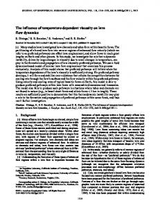
a lag in the moulting of the individuals, and to change the steepness of the moulting rate function on its early ages side. A good fit of transformed GDF is obtained with fixed values of a (r2 > 0.95). Figure 1A and B shows the results of the fit of the simple parameterization to the output data from the process model 'CS' for copepodid stages Cl and Cl. The Stage Cl

2 20°C

Downloaded from http://plankt.oxfordjournals.org/ by guest on January 2, 2012

C

2n

k

1-

0 -

h

"\

20°C

20°C

' i ' r*?T ' i ' i

1

i

12 3 4 5 6 7 Age classes (days)

' i

0 12 3 4 5 6 7 Age classes (days)

Fig. L Transfer rate function for E.acutifrons:fitof modified gamma density function to the output of a population model ('CS') for two copepodid stages. (A-C) Copepodid Cl; (D-F) copepodid Cl. (A, D) The difference in the transfer function of the two stages appears in the early ages. At 12°C, for instance, the rate of moulting of Cl increases later than in the next stage C2. The consequence is a large value of a in equation (3) for stage Cl. (B, E) Shape of the transfer function for different temperatures at a constant food concentration. (C, F) Shape of the transfer function for different food concentrations at a constant temperature.

1335

S-Sooissi, F.Carlotti and P.Nival

Table IL Euterpina acutifrons. (A) Mean and SD of V and o [equation (5)] in the range 3-11 umol N H of the first fit of parameter b to food concentration. (B) Values of parameters X and 8 of parameter •*• [equation (6)] of the second fit to temperature assuming u> constant (0.5). (C) Values of parameters X, 8 and ID from the fit of equation (7) for all developmental stages (A) Stage

CO

(day-') Mean

SD

Mean

SD

5.46 4.24 3.25 3.26 3.95 3.54 7.22 2.80 4.04 3.26 6.15 4.29

1.34 1.01 0.81 0.87 1.07 0.95 1.92 0.67 1.09 0.78 1.51 1.74

0.51 0.52 0.50 0.48 0.48 0.48 0.48 0.51 0.48 0.51 051 050

0.04 0.04 0.05 0.05 0.05 0.05 0.05 0.06 0.05 0.05 0.05 0.05

(B) Stage

Nl N2 N3 N4 N5 N6 Cl C2 C3 C4 C5

V (co = 0.50) X (°C-' d a y 1 )

8 (day 1 )

0.32 0.24 0.19 0.20 0.25 0.23 0.46 0.16 0.26 0.19 036

-0.55 -0.21 -0.40 -0.61 -0.88 -0.78 -1.50 -0.29 -0.95 -0.29 -0.74

X (°C-' day- 1 )

8 (day 1 )

[(umol N)- 1]

031 0.24 0.19 0.20 0.25 0.23 0.45 0.16 0.26 0.19 0.36

-054 -0.27 -038 -0.65 -0.88 -0.76 -1.42 -028 -0.92 -0.27 -0.67

0.53 054 052 050 050 0.50 059 0.53 050 0.53 053

(Q Stage Nl N2 N3 N4 N5 N6 Cl C2 C3 C4 C5

1336

r2 1

0.996 0.996 0.995 0.994 0.994 0.994 0.996 0.996 0.994 0.996 0.996

Downloaded from http://plankt.oxfordjournals.org/ by guest on January 2, 2012

Nl N2 N3 N4 N5 N6 Cl C2 C3 C4 C5 All stages

[(umol N)-']

Food, temperature and moulting rates

time to reach maximum transfer rate and mean duration of stages were longer at low than at high temperatures. Figure IB, C, E and F shows the transfer function under the effect of temperature at optimal food concentration (8 umol N H) and of different food concentrations at 20°C. Variation of parameter b with food and temperature Vidal (1980) has shown that mean development time (u) is related to food concentration (F) in the following way:

b = ^(1 - e-"15)

(5)

As the shape of this curve does not vary strongly with temperature, we assigned a constant value to the shape parameter (to). The elevation of curves depending on the value of ¥ should be related to temperature. We assume, as a first approximation, that ^ varies linearly with temperature. (6) Combining equations (5) and (6), an expression for b(T,F) is obtained: e^ f )

(7)

The simplex minimization algorithm given with the optimization functions of MATLAB software was used to determine the parameters of equation (3), (5), (6) or (7). Fitting a function to a set of data is based on the minimization of the sum of the squares of deviation between computed and measured values. In some cases where variance in measurements is high, the optimization procedure cannot find the absolute minimum in the parameter space. In this case, it is necessary to proceed by steps. For instance, fitting equation (5) for separate temperature values and afterward, assuming co constant, fitting equation (6). Table IIA gives the mean values of ¥ and w after fitting equation (5), for each temperature, to varies only slightly, with a mean value of 0.5 (SD = 0.05) for all stages. This observation satisfies the assumption made previously. Assigning the constant value 0.5 to w, we fitted equation (6) to ¥ (Table IIB). Figure 2 shows that the linear relationship represents the variations of ¥ versus temperature. The slope X is greater in stage Cl than in stage C2. Table IIC gives the values of to, X and 8 after fitting directly equation (7). The values are not very different from those obtained previously in two steps. The variation of b versus food and temperature is given by Figure 3 for two developmental stages: Cl with a high value of a (9) and C2 with a low value of a 1337

Downloaded from http://plankt.oxfordjournals.org/ by guest on January 2, 2012

Equation (4) shows that b is inversely proportional to u, so we suggest using the following function:

S-Souissi, F.Carlotti and P.Nival

10 -, 9 8 7 6 5 4 3 2 10

12

14

16

18

20

22

24

26

28

Temperature (°C) Fig. 2. The linear approximation of temperature effects on ¥ [equation (3)] in the range 12-26°C.

(3). b is larger for high temperature and high food. Isolines show that the same b can be found for different combinations of food concentration and temperatures. Variation of median age and standard deviation of moulting rate with food and temperature The median age (MA) is located between tM [equation (3)], the time corresponding to the maximum of transfer rate (mode), and u [equation (3)], the mean development time: - = 0.0053 (jig C)" 1 1; i2 = 0.845] to the inverse of naupliar duration of T.battagliai. Data are from Williams and Jones (1994).

1344

Downloaded from http://plankt.oxfordjournals.org/ by guest on January 2, 2012

The same expression [equation (7)] adequately fits the development of four copepodid stages of C.pacificus obtained by Vidal (1980). An estimation of the parameters (w, X, 5) was obtained from the fit of equation (7) to the data of Williams and Jones (1994) for naupliar stage duration (Figure 8). Equation (4) shows that the square of b is inversely proportional to the variance of the development time. As b increases with food concentration, the variance should decrease with food and temperature. Such a trend can be found in the results of Williams and Jones (1994). Their Table 3 gives the standard deviations of copepodid stage durations of T.battagliai for high food and high temperature. At their lowest experimental food condition, the low transfer rates predicted from our function are not observed because mortality increases. Carlotti and Sciandra (1989) have shown that a shortage in food can increase the spread of the stage-frequency curve (see their Figure 11). With the same mean transfer rate, the individuals can be highly synchronous (low dispersion) or not synchronous at all (large dispersion). If the variance in transfer rate in a stage is small, all the individuals are moulting at nearly the same time, so the population will be dominated by one stage. Cohorts will be easy to identify. On the contrary, if the variance is large, moulting will be distributed over a large interval of time and different stages will occur simultaneously. Successive cohorts will merge and the population will rapidly reach a stable structure. We can formulate the hypothesis that in environments with low food levels and low temperature, copepod populations will display a stable structure. In environments with high

Food, temperature and moulting rates

Acknowledgements This work was made possible by a CNRS grant to S.Souissi. Additional funding was provided by the Commission of the European Communities under contract MAS2-CT93-0057 of the MAST-II programme and GLOBEC France-PNDR programme. The authors thank Patrick Chang for improving the English. References Ban,S. (1994) Effect of temperature and food concentration on post-embryonic development, egg production and adult body size of calanoid copepod Eurytemora a/finis. J. Plankton Res., 16, 721-735. Carlotti^F. and Nival,S. (1991) Individual variability of development in laboratory-reared Temora stylifera copepodites: consequences for the population dynamics and interpretation in the scope of growth and development rules. / Plankton Res., 13, 801-813. Carlotti,F. and Nival,P. (1992a) Model of copepod growth and development: moulting and mortality in relation to physiological processes during an individual moult cycle. Mar. EcoL Prog. Ser., 84, 219-233. Carlotti J\ and Nival,S. (1992b) Moulting and mortality rates of copepods related to age in stage: experimental results. Mar. EcoL Prog. Ser., 84, 235-243. Carlotti,F. and Sciandra,A. (1989) Population dynamics model of Euterpina acutifrons (Copepoda: Harpacticoida) coupling individual growth and larval development. Mar. EcoL Prog. Ser, 56, 225-242. Davis.C.S. (1984) Predatory control of copepod seasonal cycles on Georges Bank. Mar. BioL, 82, Devroye,L. (1986) Non-Uniform Random Variate Generation. Springer-Verlag, New York. Klein Breteler.W.C.M. and Schogt,N. (1994) Development of Acartia clausi (Copepoda, Calanoida) cultured at different conditions of temperature and food. In Ferrari,F.D. and Bradley.B.P. (eds). Ecology and Morphology of Copepods. Kluwer Academic Publishers, Dordrecht, Vol. 297/298, pp. 469-479. Klein Breteler.W.C.M., Fransz^.G. and Gonzalez^.R. (1982) Growth and development of four calanoid copepod species under experimental and natural conditions. Neth. J. Sea Res., 16,195-207.

1345

Downloaded from http://plankt.oxfordjournals.org/ by guest on January 2, 2012

food and high temperature, a copepod population will display successive generations and cohorts. However, these conditions are not very often found simultaneously, except in eutrophicated areas. If temperature is higher than the optimal value, it will slow down the development or increase mortality. Our model for b does not take into account this situation, but it is possible to replace the linear relationship with temperature [equation (6)] by another more appropriate one. This parameterization of moulting rates, with a simple function of age in a stage, gives the possibility of including population dynamics in models of ocean circulation. This function is convenient in environments which vary slowly and are spatially homogeneous. This procedure will be limited in highly variable environments because it does not take into account the buffering properties of the matter budget of organisms. The model presented here can be used, for instance, to simulate the time variation of copepod prey of a target fish species, instead of having a forcing function. It allows a link between environmental conditions (temperature, phytoplankton concentration) and the target species, with less computer time than using a complete food chain and population dynamic models.

S^onissi, F.Cariotti and PJNival

Received on July 20, 1996; accepted on May 15,1997

1346

Downloaded from http://plankt.oxfordjournals.org/ by guest on January 2, 2012

Klein Breteler,W.C.M., Schogt,N. and van der MeerJ. (1994) The duration of copepod hie stages estimated from stage-frequency data. / Plankton Res., 16,1039-1057. Klein Breteler,W.C.M., Gonzalez,S.R and SchogtJV. (1995) Development of Pseudocalanus elongatus (Copepoda, Calanoida) cultured at different temperature and food conditions. Mar. EcoL Prog. Set, 119, 99-110. Klekowski^R.Z. and Duncan^A. (1975) Physiological approach to ecological energetics. In Grodzinski.W., Klekowski^R-Z. and Duncan,A- (eds), Methods for Ecological Bioenergetics. Blackwell Scientific, Oxford, Vol. 24, pp. 15-64. Landry,M.R. (1975) The relationship between temperature and the development of life stages of the marine copepod Acartia clausi Gisbr. LimnoL Oceanogr., 20, 854-858. Miller.C.B., Huntley,M.E. and Brooks,E.R. (1984) Post-collection moulting rates of planktonic, marine copepods: measurement, application, problems. LimnoL Oceanogr, 29,1274-1289. ReadJCL.Q. and Ashford J.R. (1968) A system of models for the life cycle of a biological organism. Biometrika, 55, 211-221. SciandraA. (1986) Study and modelling of development of Euterpina acutifrons (Copepoda, Harpacticoida). / Plankton Res., 8,1149-1162. VidalJ. (1980) Physioecology of zooplankton. n. Effects of phytoplankton concentration, temperature, and body size on the development and molting rates of Calanus pacificus and Pseudocalanus sp. Mar. BioL, 56,135-146. Williams.T.D. and Jones,M.B. (1994) Effects of temperature and food quantity on postembryonic development of Tisbe battagliai (Copepoda: Harpacticoida). / Exp. Mar. BioL EcoL, 183,283-293. Wroblewski,J.S. (1980) A simulation of the distribution of Acartia clausi during Oregon Upwelling, August 1973. J. Plankton Res., 2,43-68.