For ideal fluids, Eulerian and Lagrangian instabilities are equivalent. Stephen C. Preston. September 4, 2003. Contents. 1 Introduction. 1. 2 Geometry of D(M) ...
For ideal fluids, Eulerian and Lagrangian instabilities are equivalent Stephen C. Preston September 4, 2003
Contents 1 Introduction
1
2 Geometry of D(M ) and Dµ (M ) 2.1 The diffeomorphism group . . . . . . . . . . . . . . . . . . . . . . 2.2 The volume-preserving diffeomorphism group . . . . . . . . . . . 2.3 The splitting of the Jacobi equation . . . . . . . . . . . . . . . .
3 3 4 6
3 Explicit solutions of the Jacobi equation
7
4 Asymptotic growth of Jacobi fields
11
5 Conclusion
17
1
Introduction
The motion of an incompressible fluid filling up a domain may be studied from two perspectives: either by considering the time-dependent velocity field, or by considering the paths followed by each fixed fluid particle. The first approach is the Eulerian view, while the second is the Lagrangian view. Although the two approaches are equivalent (since the velocity field may be integrated to determine the flow), they lead to different forms of the equations. These differences lead to two notions of stability: the Eulerian and the Lagrangian. Loosely speaking, if the initial velocity field is perturbed, a fluid motion which is stable in the Eulerian sense will have its velocity field remain close to the unperturbed state, while a motion which is stable in the Lagrangian sense will have particle paths remaining close to the unperturbed paths. We are interested in the connection between these two notions. More specifically we look at linearizations of the fluid equations and estimate the growth in time of solutions. If all Eulerian perturbations are bounded in time, in some norm, the fluid motion is Eulerian stable. If all Lagrangian perturbations are bounded, the fluid motion is Lagrangian stable. We can also 1
distinguish types of instability: a fluid motion is called (Eulerian or Lagrangian) polynomially unstable if all perturbations grow at most polynomially in time; it is exponentially unstable if at least one perturbation grows exponentially in time. Many aspects of Eulerian stability had been well understood by the late 1800s, thanks to the efforts of Lord Rayleigh and others. By contrast, much less was known about Lagrangian stability until 1966, when Arnold [1] discovered a geometric approach to the field. Arnold showed that an incompressible fluid traces out a geodesic in the group of volume-preserving diffeomorphisms, Dµ (M ), of its domain M . Thus infinitesimal Lagrangian perturbations are Jacobi fields along this geodesic. Arnold suggested that the sign of the curvature could therefore be used to predict Lagrangian instability, as quoted in Arnold-Khesin [2] (Chapter IV, Remark 4.3): “One can expect that the negative curvature of the diffeomorphism group causes exponential instability of geodesics (i.e. flows of the ideal fluid) in the same way as for a finite-dimensional Lie group.” The geometry of the volume-preserving diffeomorphism group was originally studied using general techniques of one-sided invariant metrics on Lie groups. In the past decade, the use of submanifold geometry has facilitated many new results; see for example Bao-Lafontaine-Ratiu [3] or Misiolek [8]. In Section 2 we review the geometry of the full diffeomorphism group D(M ), along with the geometry of Dµ (M ) as a submanifold of D(M ). The major result of Section 2 is Proposition 2.4, which says that the Jacobi equation on Dµ (M ) splits into two decoupled first-order partial differential equations: the standard linearized Euler equation, and the linearized flow equation, an analogue of the dynamo equation of magnetohydrodynamics. In Section 3, we use this decoupling to give a counterintuitive example of the connection between curvature and stability, by finding explicit formulas for the Jacobi fields along the geodesic generated by plane parallel Couette flow on the cylinder [0, π] × S 1 . Plane parallel Couette flow has a nonpositive curvature operator along its corresponding geodesic, with strictly negative curvature in many directions. Thus one would expect Jacobi fields to grow exponentially. However, we find that in fact all Jacobi fields grow at most linearly in time at each point of M . We conclude that the sign of the curvature of Dµ (M ) does not reliably predict the asymptotic growth rate of Jacobi fields, and thus that it cannot be used as a criterion for Lagrangian stability. In fact, it turns out that Eulerian instability and Lagrangian instability are very closely related, as we demonstrate in Section 4 for the two-dimensional case. The decoupling of the Jacobi equation establishes a relationship between Jacobi fields and linear Eulerian perturbations. We use this relation to show that if all Eulerian perturbations are bounded, then no Jacobi field can grow more than quadratically with time, in the L2 norm—the natural Riemannian metric on the diffeomorphism group. Thus it is impossible to have an Eulerian stable flow that is exponentially Lagrangian unstable. The general principle in two dimensions is that a given fluid flow either has 2
1. at most polynomial instability in both the Eulerian and the Lagrangian senses, or 2. exponential instability in both the Eulerian and Lagrangian senses. Similar results are valid in the three-dimensional case. The techniques are essentially the same and thus for simplicity we have focused on the twodimensional case. For general background information on the subject, we highly recommend the recent text of Arnold-Khesin [2]. We will need a number of basic facts about Riemannian geometry; do Carmo [4] is a good reference for this material and we will use the notation of that book. Much of this research was conducted while the author pursued graduate studies at the State University of New York at Stony Brook, and portions were published in the author’s dissertation [10]. The author would like to thank David G. Ebin, Gerard Misiolek, and Herman Gluck for advice and useful discussions.
2 2.1
Geometry of D(M ) and Dµ (M ) The diffeomorphism group
The group of diffeomorphisms, under composition, of a manifold M is denoted D(M ). The geometrical properties of D(M ) are very closely related to those of M itself. This space is the ambient manifold for the configuration space D µ (M ) for ideal fluid dynamics, so it is worth understanding in depth. For simplicity we will assume all objects are C ∞ . At a diffeomorphism η ∈ D(M ), the tangent space Tη D(M ) consists of elements U ◦ η, where U is a vector field on M . If h·, ·i is the Riemannian metric on M and µ is the corresponding volume form, the Riemannian metric hh·, ·ii on Tη D(M ) is given by the formula Z hU, V i◦η µ, for any vector fields U and V . (2.1) hhU ◦η, V ◦ηii = M
Given a vector field X on M , we may construct a right-invariant vector field X on D(M ) by defining Xη = X ◦η for each η ∈ D(M ). The covariant derivative of right-invariant vector fields satisfies � ∇X Y η = (∇X Y ) ◦ η. (2.2)
One consequence of equation (2.2) is that the curvature tensor R of D(M ) satisfies Rη (X, Y)Z = R(X, Y )Z ◦ η. (2.3) See Misiolek [8] or Bao-Lafontaine-Ratiu [3] for details and references. As another consequence, we have the following formula for the covariant derivative of a vector field along a curve. 3
Proposition 2.1. If η : (−ε, ε) → D(M ) is a smooth curve, and we define a vector field X(t) by the formula ∂η = X(t)◦η(t), ∂t then the covariant derivative of a right-translated vector field Y (t)◦η(t) along η is � � � ∂Y D� + ∇X(t) Y (t) ◦ η, (2.4) Y (t)◦η(t) = ∂t ∂t
2.2
The volume-preserving diffeomorphism group
The configuration space of an incompressible fluid is Dµ (M ), the submanifold of D(M ) consisting of diffeomorphisms η satisfying η ∗ µ = µ, where µ is the Riemannian volume form. At any η, the elements of the tangent space Tη Dµ (M ) are of the form X ◦η, where X is divergence-free and tangent to the boundary. The L2 metric (2.1) on D(M ) induces a metric on Dµ (M ) defined by Z Z hhU ◦η, V ◦ηii ≡ hU, V i◦η µ = hU, V i µ. M
M
This induced metric is right-invariant. An arbitrary vector field (not necessarily tangent to ∂M ) can be orthogonally projected onto the space of divergence-free vector fields tangent to the boundary using the Hodge decomposition. Given a vector field X, we solve the Neumann boundary value problem ∆f = div X, h∇f, n ˆ i ∂M = hX, n ˆ i ∂M
to obtain a function f , unique up to a constant, and then define the orthogonal projection P(X) as P(X) = X − ∇f. (2.5)
By construction, P(X) is divergence-free and tangent to the boundary. The covariant derivative on the submanifold Dµ (M ) is the projection of the covariant derivative on the larger manifold D(M ). So the geodesic equation on Dµ (M ) is given by � � e ∂η D ∂η D ≡P = 0. (2.6) ∂t ∂t ∂t ∂t Using formula (2.1), the geodesic equation (2.6) may be decoupled into the two equations ∂η − X(t)◦η(t) = 0 ∂t � ∂X + P ∇X(t) X(t) = 0. ∂t 4
(2.7) (2.8)
For smooth initial data η(0) and X(0), Ebin-Marsden [5] proved that these equations have local solutions that are smooth in time and space. Equation (2.7) is called the flow equation, which relates the Eulerian description X(t) to the Lagrangian description η(t). Equation (2.8) is the incompressible Euler equation. Its independence from η reflects the right-invariance of the metric on Dµ (M ). The second fundamental form of the immersion of Dµ (M ) into D(M ) is given by the formula B(X, Y ) = ∇X Y − P(∇X Y ) = −∇pXY ,
(2.9)
where the function pXY is the solution of the Neumann problem ∆pXY = − div (∇X Y ), h∇pXY , n ˆ i ∂M = −h∇X Y, n ˆ i ∂M
and X and Y are divergence-free vector fields tangent to ∂M . If X is the velocity field of an incompressible fluid flow, then the function pXX gives the pressure of the fluid. We can use this notation to write the Euler equation (2.8) more explicitly as ∂X + ∇X X = −∇pXX . ∂t
(2.10)
If X does not depend on time, then it satisfies the steady Euler equation, ∇X X = −∇pXX .
(2.11)
Geodesics which start at the identity in the direction of a steady Euler flow form 1-parameter subgroups of Dµ (M ). From the second fundamental form (2.9) and formula (2.3) for the curvature e of D(M ), we can use the Gauss-Codazzi formula to compute the curvature R of Dµ (M ).
Proposition 2.2. If W , X, Y , and Z are divergence-free vector fields on M e of Dµ (M ) at the identity id ∈ Dµ (M ) is tangent to ∂M , then the curvature R given by e hhR(X, Y )Z, W ii =
Z
hR(X, Y )Z, W i µ Z Z YZ XW h∇pXZ , ∇pY W i µ. h∇p , ∇p iµ − +
M
(2.12)
M
M
e Corollary 2.3. The curvature R(X, Y )Z may be written as
� e R(X, Y )Z = P R(X, Y )Z + ∇X ∇pY Z − ∇Y ∇pXZ .
5
(2.13)
Proof. Since ∇pXW is the orthogonal projection of the vector field −∇X W onto the space of gradients, we have Z Z YZ XW h∇pY Z , ∇X W i µ h∇p , ∇p iµ = − M M Z Z h∇X ∇pY Z , W i µ Xh∇pY Z , W i µ + =− M Z M YZ h∇X ∇p , W i µ, = R
M
where we used the fact that M X(f ) µ = 0 for any divergence-free vector field X tangent to ∂M and any function f . Performing the same simplification on the other term of (2.12), we get Z e hhR(X, Y )Z, W ii = hR(X, Y )Z + ∇X ∇pY Z − ∇Y ∇pXZ , W i µ M
and formula (2.13) follows since W was arbitrary.
2.3
The splitting of the Jacobi equation
The curvature appears in the Jacobi equation on Dµ (M ) along a geodesic η with velocity field X: e e D � � D e Y (t), X(t) X(t) ◦ η = 0, Y (t)◦η(t) + R ∂t ∂t
(2.14)
where Y (t) ◦ η(t) is a geodesic deviation along η. Misiolek [8] proved that equation (2.14) has a unique smooth solution for given smooth initial data Y (0) e and DY ∂t t=0 . The Jacobi equation (2.14) is obtained by the standard procedure of linearization of the geodesic equation. However we can also linearize the equations (2.7) and (2.8) directly. Proposition 2.4. Suppose that for each fixed s, the curve t 7→ η(t, s) is a geodesic in Dµ (M ) with η(0, s) = id, and that X(t, s) satisfies ∂η = X(t, s) ◦ η(t, s). ∂t Then the linearizations Y (t) and Z(t) defined by ∂η ∂X Y (t) ◦ η(t, 0) ≡ and Z(t) ≡ ∂s s=0 ∂s s=0
satisfy the linearized geodesic equations
∂Y + [X(t), Y (t)] = Z(t) ∂t � ∂Z + P ∇X(t) Z(t) + ∇Z(t) X(t) = 0. ∂t 6
(2.15) (2.16)
In addition, the linearized geodesics equations (2.15) and (2.16), with initial conditions Y (0) = 0 and Z(0) = Z0 , are equivalent to the Jacobi equation (2.14), e with initial conditions Y (0) = 0 and DY ∂t t=0 = Z0 . Proof. We derive (2.15) and (2.16) simply by differentiating equations (2.7) and (2.8) with respect to s. That these equations are equivalent to the Jacobi equation follows from the fact that equations (2.7) and (2.8) are equivalent to the geodesic equation, and the fact that we are using the same linearization procedure along η. It is also instructive to perform the calculation directly, by using (2.15) as a formula for Z and plugging in to (2.16). Using the formula � � e � D ∂Y XY + ∇X Y + ∇p ◦η(t) Y (t)◦η(t) = ∂t ∂t
e we can check for the covariant derivative and formula (2.13) for the curvature R, that the partial differential equations are identical. Proposition 2.4 was also proved by Rouchon [11], who used it to compute the curvature (2.13) that we derived from the Gauss-Codazzi formula. The equation (2.16) is the usual linearized Euler equation, typically studied for a time-independent steady flow X. Equation (2.15) is a nonhomogeneous version of the equation ∂Y + [X(t), Y (t)] = 0, (2.17) ∂t which in magnetohydrodynamics is called the “fast dynamo equation.” (See Arnold-Khesin [2] for details.) In general, the linearized flow equation is fairly easy to solve explicitly, while the linearized Euler equation is far more difficult. But it can be done in some very special cases, as we will show in the next section.
3
Explicit solutions of the Jacobi equation
In this section we compute Jacobi fields explicitly, using the splitting in Proposition 2.4. In what follows we will always suppose the initial conditions on the e Jacobi field are Y (0) = 0 and DY ∂t |t=0 6= 0, which follows from the assumption that geodesics start at the identity. One of the simplest flows for which there is an explicit solution of the linearized Euler equation is plane parallel Couette flow, given by the formula X = x ∂y on the flat cylinder M = [0, π] × S 1 . The choice 0 ≤ x ≤ π is not important but it makes formulas simpler. Because we have ∇X X = 0, the function pXX is constant. Thus by formula (2.12), for every divergence-free Y tangent to the boundary of M , we have Z e h∇pXY , ∇pXY i µ ≤ 0, hhR(Y, X)X, Y ii = − M
7
and this is strictly negative if ∇pXY 6= 0. Since ∆pXY = − div (∇Y X) = −
∂Y 1 , ∂y
the curvature is strictly negative unless Y = v(x) ∂y for some function v. Despite the nonpositivity of the curvature operator, we find that there are no exponentially growing Jacobi fields. Theorem 3.1. Suppose X = x ∂y is plane parallel Couette flow on the flat cylinder M = [0, π] × S 1 , and that Y (t) is a Jacobi field along the corresponding e geodesic in Dµ (M ) with initial conditions Y (0) = 0 and DY ∂t t=0 = Z(0). Then |Y (t)| = O(t) at every point of M . Proof. We first solve the linearized Euler equation. The solution of (2.16) was first presented by Orr [9], and we will repeat the derivation in order to then solve for the Jacobi field. Let us write Z = h ∂x + j ∂y . We first expand h and j in a Fourier series in y: ∞ ∞ X X jn (t, x)einy . hn (t, x)einy , j(t, x, y) = h(t, x, y) = n=−∞
n=−∞
Then the condition div Z = 0 translates into the equation ∂hn + injn = 0 for every n. ∂x
(3.1)
If n 6= 0, this determines jn in terms of hn . The condition that Z remains tangent to the boundary translates into the requirements that hn (t, 0) = 0 and hn (t, π) = 0, for all t.
(3.2)
The linearized Euler equation (2.16) can be written as ∂Z + ∇X Z + ∇Z X = −2∇q. ∂t The function q can also be expanded as a Fourier series in y, and we find that h and j satisfy ∂hn ∂qn + inxhn = − ∂t ∂x ∂jn + inxjn + hn = −inqn . ∂t
(3.3)
For n = 0, equation (3.1) along with the boundary conditions (3.2) immediately imply that h0 (t, x) ≡ 0. Then equations (3.3) imply that j0 (t, x) = j0 (0, x).
8
So in what follows we will assume n 6= 0. Eliminating qn from equations (3.3), we obtain � � 2 � � ∂ ∂ 2 hn ∂ hn 2 2 − n hn + inx − n hn = 0. (3.4) ∂t ∂x2 ∂x2 The first step to solve equation (3.4) is writing � 2 � ∂ hn ∂ 2 hn 2 −inxt 2 (t, x) − n hn (t, x) = e (0, x) − n hn (0, x) . ∂x2 ∂x2
(3.5)
To proceed further, it helps to expand hn (0, x) in a Fourier sine series, using the conditions (3.2). We will work with each component individually; then we can use linearity to add the solutions. So suppose hn (0, x) =
2i sin (mx), for some integer m, m2 + n 2
the coefficient being chosen to simplify later formulas. For fixed t, equation (3.5) is an ordinary differential equation in x, and the explicit solution may be obtained by standard methods. We get imx −inxt −imx −inxt 1 1 hn (t, x) = (m−nt) e − (m+nt) e 2 +n2 e 2 +n2 e � � � sinh n(π − x) + (−1)m e−inπt sinh nx� 1 1 − (m−nt) . 2 +n2 − (m+nt)2 +n2 sinh (nπ) (3.6)
From the divergence-free condition (3.1), we can obtain a formula for jn (t, x). We can see that hn asymptotically grows like O(1/t2 ), while jn asymptotically grows like O(1/t) at every point. Our real interest, however, is in the Jacobi field Y , which we find by solving equation (2.15). Writing Y = f ∂x +g ∂y , we proceed as before. First we expand f and g in Fourier series in y: f (t, x, y) =
∞ X
fn (t, x)einy ,
g(t, x, y) =
∞ X
gn (t, x)einy .
n=−∞
n=−∞
Again the divergence-free condition implies that ∂fn + ingn = 0, ∂x
(3.7)
so we only need to solve for fn . The horizontal component of (2.15) is ∂fn + inxfn = hn , ∂t
9
(3.8)
whose solution with fn (0, x) ≡ 0 is Z t fn (t, x) = hn (s, x)einx(s−t) ds. 0
Using equation (3.6), we get Z t 1 1 e−imx ds − ds m 2 m 2 2 n 0 (s − n ) + 1 0 (s + n ) + 1 � � sinh n(π − x) pm,n (t, x) + (−1)m sinh nx pm,n (t, x − π) , − n2 sinh (nπ)
f (t, x)einxt =
eimx n2
Z
t
(3.9)
where pm,n (t, x) =
Z t� 0
1 1 − m 2 2+1 ) (s − m (s + n n) +1
�
einxs ds.
(3.10)
To determine the asymptotic behavior of Y for large t, we first need to find an asymptotic expansion for fn . We can easily derive the asymptotic expansions for the first two integrals in (3.9): Z t �1� 1 π 1 ds = − arctan c − + O . (3.11) 2 2 t t2 0 (s + c) + 1 We get an asymptotic expansion for pm,n , defined by (3.10), as follows: � Z ∞� 1 1 einxs ds pm,n (t, x) = − 2 2 (s − m (s + m 0 n) +1 n) +1 Z ∞ inxs 4m n se − ds 2 m2 2 2 (s2 − m t n2 ) + 2(s + n2 ) + 1 �1� = pm,n (∞, x) + O 2 , t
where pm,n (∞, x) is defined as the improper integral (a half-Fourier transform). Thus we can write � � �1� 2i fn (t, x) = α(x) − 2 sin (mx) e−inxt + O 2 , (3.12) n t t
where α(x) ≡
� � 1� m cos (mx) iπ sin (mx) + 2 arctan n n2 � � sinh n(π − x) pm,n (∞, x) + (−1)m sinh nx pm,n (∞, x − π) − . n2 sinh (nπ)
So for large time and fixed x, fn (t, x) is approximately sinusoidal with period 2π nx and complex amplitude α(x). 10
frag replacements
0.5
0
t
−0.25 0.25
6
� � Re gn (t, x0 )einx0 t
1
2
3
4
5
Figure 3.1: The real part of the amplitude of gn (t, x0 ), plotted against time, for π the case n = 1, m = 2, � and x0 = 3 . For comparison, the linear approximation i 0 Re α(x0 )t + n α (x0 ) is also shown. From the asymptotic expansion (3.12) of fn , we obtain an asymptotic expansion for gn using formula (3.7): � � �1� 2 i . (3.13) gn (t, x) = α(x)t + α0 (x) − sin (mx) e−inxt + O n n t So the vertical component of the Jacobi field grows linearly in time at each point. A typical plot of gn (t, x) is shown in Figure 3.1. The important point is obviously that the Jacobi fields do not grow expoe nentially, despite the fact that the curvature hhR(Y, X)X, Y ii is negative for most vector fields Y and zero for the rest. This is quite counterintuitive, and no similar phenomenon is known in finite-dimensional Lie groups.
4
Asymptotic growth of Jacobi fields
In this section we study the growth of Jacobi fields along geodesics in D µ (M 2 ) which are generated by steady solutions of the Euler equation. We show that if all linear Eulerian perturbations grow polynomially in time, then so do all Jacobi fields in the L2 norm. At the end of the section we mention analogous results for the three-dimensional case. We first need two lemmas.
11
Lemma 4.1. If X is a divergence-free vector field on a surface M , and we define a vector field W by the formula W =
1 ?X, hX, Xi
(4.1)
where ? is the operation of rotation by 90◦ in each tangent space, then the Lie bracket [X, W ] satisfies [X, W ] = ξX (4.2) for some function ξ. Proof. To verify equation (4.2), we only need to show that h?X, [X, W ]i ≡ 0. We have h?X, [X, W ]i = h?X, ∇X W i − h?X, ∇W Xi 1 h?X, ∇?X Xi = hX, Xi hW, ∇X W i − hX, Xi 1 1 hX, ∇X Xi − h?X, ∇?X Xi =− hX, Xi h?X, ?Xi = − div X = 0. Thus [X, W ] is proportional to X. Lemma 4.2. Suppose X is a divergence-free vector field on a surface M , tangent to ∂M . Let q be some time-dependent function on M , and let p be the solution of the equation ∂p + X(p) = q, ∂t
p(0) = 0.
(4.3)
Then the L2 norms of p and q are related by Z t kq(s)k ds kp(t)k ≤ 0
Proof. Let η(t) be the flow of X. Then since X is divergence-free, η(t) is volumepreserving. Since equation (4.3) can be written as
its solution is
� ∂� p(t)◦η(t) = q(t)◦η(t), ∂t p(t) =
Z
t 0
q(s)◦η(s − t) ds.
12
Therefore the L2 norm of p can be estimated using the Schwartz inequality: Z Z tZ tZ h i h i 2 p (t) µ = q(s)◦η(s − t) · q(σ)◦η(σ − t) µ ds dσ 0 M 0 M � �q � Z t Z t �q R R 2 2 q (s)◦η(s − t) µ · q (σ)◦η(σ − t) µ ds dσ ≤ M M 0
0
=
�Z t q R
q 2 (s)◦η(s − t) µ ds M
0
�2
=
�Z
t
0
kq(s)k ds
�2
,
where in the last line we used the change of variables formula and the fact that η(s − t)∗ µ = µ. The lemma follows on taking square roots. Theorem 4.3. Suppose X is a divergence-free vector field on a two-dimensional compact manifold M , with no stagnation points. Then if Y and Z are solutions of equations (2.15) and (2.16) with Y (0) = 0, then the L2 norms of Y and Z satisfy Z p supM |X| t 2 2 kZ(s)k ds, (4.4) kY (t)k ≤ 3 + 2A t inf M |X| 0 for some constant A. In particular, if the L2 norm of Z is bounded for all time, then the L2 norm of Y grows at most quadratically in time. Proof. Suppose we are given a solution Z(t) of the linearized Euler equation (2.16). We define W by equation (4.1), and write Y and Z in terms of the basis {W, X} as Z(t) = h(t)W + j(t)X
and
Y (t) = f (t)W + g(t)X.
Then by Lemma 4.1, we can write the linearized flow equation (2.15) in components as � ∂g +X g +ξf = j ∂t � ∂f +X f =h ∂t Now using Lemma 4.2, we find that Z t kh(s)k ds, kf (t)k ≤ 0
and thus that kg(t)k ≤ ≤ ≤
Z
Z
Z
t
kj(s) − ξ f (s)k ds
0 t
kj(s)k ds + sup |ξ| M
0 t 0
Z
kj(s)k ds + t sup |ξ| M
13
t
kf (s)k ds
0
Z
t 0
kh(s)k ds.
R h2 µ + M hX, Xi j 2 µ, we have sZ 1 1 kjk ≤ kZk hX, Xi j 2 µ ≤ inf M |X| inf M |X| M
Since kZk2 =
R
1 M hX,Xi
and khk ≤ sup |X| M
sZ
M
1 h2 µ ≤ sup |X| kZk. hX, Xi M
Thus we can compute Z Z hX, Xig 2 (t) µ + kY (t)k2 =
1 f 2 (t) µ hX, Xi M M 1 ≤ suphX, Xikg(t)k2 + kf (t)k2 inf M hX, Xi M �2 � �2 sup |X|2 � �Z t � 1 M 2 kZ(s)k ds . + t sup |ξ| sup |X| + · ≤ sup |X| inf M |X| inf M |X|2 M M M 0 Equation (4.4) follows as desired, with
A = sup |ξ| · inf |X| · sup |X|. M
M
M
√ If kZ(s)k ≤ C for all s, then kY (t)k ≤ CKt 3 + 2A2 t2 , and thus kY (t)k = O(t2 ) as t → ∞. Remark 4.4. Although the coefficient in Theorem 4.3 is not sharp, the quadratic growth estimate of the L2 norm is, in general, the best possible. To see this, we construct the following example. Let M be the torus T2 , with a metric given by ds2 = dr2 + ϕ2 (r) dθ 2 with ϕ(r) a periodic, nowhere-zero function of r. (For example, the standard embedding of the torus in R3 gives ϕ(r) = c + d cos r, with |c| > |d|.) Let 1 ∂ . X= 2 ϕ (r) ∂θ Then P(∇X X) = 0 and div X = 0, so that X is a steady solution of the Euler equation (2.11). Define 1 ∂ Z= . ϕ(r) ∂r We have div Z = 0, and since ∇X Z + ∇Z X = 0, Z is a steady solution of the linearized Euler equation (2.16). The corresponding Jacobi field can be computed as Y (t, r, θ) =
t ∂ t2 ϕ0 (r) ∂ − 4 . ϕ(r) ∂r ϕ (r) ∂θ
(4.5)
Thus if ϕ is not constant, the Jacobi field grows quadratically in time at each point. 14
The important conclusion is that growth is polynomial in time: we have ruled out exponential growth of the Jacobi field Y unless the perturbed velocity field Z also grows exponentially in time. Arnold-Khesin [2] had suggested that “a stationary flow can be a Lyapunov stable solution of the Euler equation, while the corresponding motion of the fluid is exponentially unstable.” (Chapter IV, Remark 4.3). Theorem 4.3 shows that this is actually impossible for twodimensional flows without stationary points. A drawback of Theorem 4.3 is that it relies on X having no stagnation points, which is a severe topological restriction on the surface. However, if X does have isolated stagnation points, we can remove an X-invariant neighborhood of the points and apply Theorem 4.3 to the remaining portion of the manifold. Then we can analyze the behavior near the singularities separately. The two simplest cases are nondegenerate stationary points of elliptic and hyperbolic types. We shall see that a flow with only elliptic fixed points has no Lagrangian instability. On the other hand, a flow with a hyperbolic fixed point has an exponential Lagrangian instability, as well as an exponential Eulerian instability. Theorem 4.5. If X is an analytic vector field on a surface M with a nondegenerate elliptic stationary point, then the L2 norm of the Jacobi field Y in a neighborhood of the stationary point satisfies an estimate of the form Z t p 2 2 kY (t)k ≤ 3 + 2A t kZ(s)k ds, 0
for some constant A.
Proof. We use the fact that for any vector field of the form described, there is a system of analytic coordinates (x, y) and an analytic function f such that X = −yf (x2 + y 2 ) ∂x + xf (x2 + y 2 ) ∂y , with f (0) 6= 0; see for example Ma˜ nosas-Villadelprat [7]. We can use any Riemannian metric to estimate the L2 norm, since all metrics generate an equivalent norm and equation (2.15) does not depend on the metric components. So we may as well use the flat metric ds2 = dx2 + dy 2 . From here the analysis proceeds very much like the proof of Theorem 4.3. The difference is that hX, Xi is invariant under the flow η(t), so that we don’t need the term supM hX, Xi/ inf M hX, Xi, which is unbounded in this case. On the other hand ξ is given by ξ(x, y) =
2f 0 (x2 + y 2 ) , [f (x2 + y 2 )]2
which remains bounded in a neighborhood of 0, so that supM |ξ| is finite. On the other hand, a hyperbolic stagnation point will create exponential instability even in a small neighborhood. 15
Theorem 4.6 (Arnold-Khesin). If X is a divergence-free vector field on a surface M with an isolated nondegenerate hyperbolic fixed point, then there are Jacobi fields with exponentially growing L2 norm. Proof. The easiest way to prove this is to simply look at solutions of the decoupled Jacobi equations (2.16) and (2.15) satisfying Z(0) = 0 and Y (0) 6= 0. Thus we only need to solve the homogeneous linearized flow equation, i.e. the dynamo equation (2.17). The fact that this equation has solutions which grow exponentially in the L2 norm was demonstrated in Arnold-Khesin [2], Chapter V, Theorem 1.7. The existence of a hyperbolic fixed point not only guarantees exponential growth of the dynamo equation, but also of the linearized Euler equation itself, as proven by Friedlander-Vishik [6]. Theorem 4.7 (Friedlander-Vishik). If X is a steady solution of the Euler equation on a surface with a hyperbolic stagnation point, then there are exponentially growing solutions of the linearized Euler equation in the L 2 norm. Now we combine the results of Theorems 4.3–4.7. Theorem 4.8. Suppose X is an analytic solution of the steady Euler equation on a surface M , with only isolated nondegenerate singularities. If X is at most Eulerian polynomially unstable, then X is at most Lagrangian polynomially unstable. There are theorems analogous to Theorem 4.3 in the three-dimensional case. We recall that if X is a steady three-dimensional solution of the Euler equation (2.11), then there is a function α (the Bernoulli function) such that X ×curl X = ∇α. If α is not constant, then we can define W =
1 h∇α,∇αi
∇α.
Since h[X, W ], W i = 0
and
[X, curl X] = 0,
the vector fields {X, curl X, W } form a convenient basis to study the linearized flow equation (2.15), and we can perform an analysis very similar to the above. If α is constant, on the other hand, then curl X and X are collinear, so X is a “force-free field” in the language of magnetohydrodynamics. If X happens to have an integral of motion (that is, a function β on M such that X(β) ≡ 0, or more generally, a curl-free vector field U such that hX, U i ≡ 0), then we can again define a convenient basis by the formulas W =
1 hU,U i
U
and
V =
1 hX,Xi X
× U.
These vector fields satisfy h[X, V ], V i = 0,
h[X, V ], W i = 0,
h[X, W ], W i = 0, 16
and
h[V, W ], W i = 0.
So they also form a convenient basis. If X is an eigenfunction of the curl operator with no integral of motion, then there may not be a simple Jordan-form basis of the Lie bracket operator Y 7→ [X, Y ], and thus we could not prove any theorem like Theorem 4.3.
5
Conclusion
In this research we have tried to clarify the relationship between Eulerian instability and Lagrangian instability, using a decoupling of the Jacobi equation. Using this method, we have found an explicit counterexample to the hypothesis that negative curvature on the diffeomorphism group is responsible for exponential Lagrangian instability. Instead, we conclude that only exponential Eulerian instability can create exponential Lagrangian instability. This complements the work of Friedlander-Vishik [6], who showed that any exponential instability (even in the C ∞ norm) of the dynamo equation (2.17) will cause an exponential instability in the linearized Euler equation (2.16), in the L2 norm. In general, one expects not to be able to achieve true Lagrangian stability in the L2 norm. The Jacobi fields computed here grow at least linearly in time, while Theorem 4.3 suggests the growth could be a higher-order polynomial. However, one should distinguish between polynomial growth of Jacobi fields and exponential growth. In the case of polynomial growth, one can still predict the Lagrangian motion in a practical sense. However, if Lagrangian perturbations grow exponentially, then long-term prediction is impossible. Thus rather than distinguishing between stability and instability, one should distinguish between “slow” polynomial instability and “fast” exponential instability. It would be interesting to study extensions of these results. In our case we have dealt with two-dimensional ideal fluids, in the simple cases where the fluid flow has only isolated nondegenerate stagnation points. It is possible that other types of stagnation points would create intermediate instabilities, such as higher-order polynomial growth of Jacobi fields in the case of degenerate elliptic zeroes. Using normal form theory, one should be able to work this out in detail. The various types of stagnation points in the three-dimensional case present still more possibilities. The techniques used in this paper can also be applied to study stability in other norms besides L2 . Sobolev norms are useful in technical studies of the diffeomorphism group (as shown by work of Ebin-Marsden [5] and Misiolek [8]). In future research we will compare Sobolev norms of Jacobi fields to those of Euler perturbations, and will show that in many cases, either both grow polynomially or both grow exponentially. Thus results presented here are not special to the L2 case, but in fact apply for any reasonable definition of linear stability. All of our results have dealt with linearizations and infinitesimal perturbations. This leads to a natural question: what effects, if any, do the differences
17
in growth rates of linear perturbations have on nonlinear instability? We have shown that typically, linear perturbations will grow in time. When they become large enough that the linear approximation is no longer valid, is there still any sense in which one can distinguish different forms of Lagrangian instability? Arnold famously demonstrated nonlinear stability in the Eulerian sense for certain flows (see Arnold-Khesin [2]), but there is almost nothing known about nonlinear stability in the Lagrangian sense. We expect that this will be a stimulating area of future research.
References [1] V.I. Arnold, “Sur la geometrie differentielle des groupes de Lie de dimension infinie et ses applications a l’hydrodynamique des fluids parfaits,” Ann. Inst. Fourier (Grenoble) 16 (1966) 319–361. [2] V.I. Arnold and B.A. Khesin, Topological methods in hydrodynamics. Springer-Verlag, New York, 1998. [3] D. Bao, J. Lafontaine, and T. Ratiu, “On a nonlinear equation related to the geometry of the diffeomorphism group,” Pacific J. Math. 158 (1993) no. 2, 223–242. [4] M.F. do Carmo, Riemannian geometry. Birkh¨auser, Boston, 1993. [5] D.G. Ebin and J. Marsden, “Groups of diffeomorphisms and the motion of an incompressible fluid,” Ann. of Math. 92 (1970) 102–163. [6] S. Friedlander and M.M. Vishik, “Instability criteria for steady flows of a perfect fluid,” Chaos 2 (1992) no. 3, 455–460. [7] F. Ma˜ nosas and J. Villadelprat, “Area-preserving normalizations for centers of planar Hamiltonian systems,” J. Differential Equations 179 (2002) 625646. [8] G.K. Misiolek, “Stability of flows of ideal fluids and the geometry of the group of diffeomorphisms,” Indiana Univ. Math. J. 42 (1993) no. 1, 215– 235. [9] W. Orr, “The stability or instability of the steady motion of a perfect fluid and of a viscous fluid, part I: A perfect fluid” Proc. Roy. Irish Acad. 27 (1907) 9–68. [10] S.C. Preston, “Eulerian and Lagrangian stability of fluid motions,” Ph. D. Thesis, SUNY Stony Brook, 2002. [11] P. Rouchon, “The Jacobi equation, Riemannian curvature and the motion of a perfect incompressible fluid,” European J. Mech. B Fluids 11 (1992) no. 3, 317–336.
18