the extended energy and instead propose a Nosé-Poincaré thermostat. Langevin dynamics produces an NVT ensemble. NAMD notes. Langevin dynamics with ...
c
Robert D. Skeel, 2003
Force Evaluation, Integrators, and Propagators1 Robert D. Skeel Department of Computer Science and Beckman Institute, University of Illinois at Urbana-Champaign
1
Introduction
Presented here is a guide to selected algorithms deemed to be useful for a subset of calculations needed for biomolecular simulations. It is beneficial to make a clear distinction between what we want to compute (model) and how we compute it (method). What we compute is the more important consideration, and this is reviewed in Section 2 under the heading “Models and aims.” How we compute it is the subject of the remaining sections. The distinction is made on the following basis: (i) uncontrolled approximations such as force fields are deemed to be part of the model and (ii) controlled approximations such as numerical integrators are classified as algorithms. Ideally, only advanced users should be conscious of algorithms; general users should merely choose error tolerances and confidence levels with the algorithms automatically chosen for them by the software. Discussed in Sections 3–5 are algorithms for the three tasks given in the title of this article. Not discussed here are force calculations based on quantum mechanics or elasticity and “protocols” that employ integrators for kinetics and propagators for sampling. An excellent reference is the 2002 book by Schlick [20] and a good supplement is the 1987 book of Allen and Tildesley [1]. Also noteworthy is the biologically-oriented book by Leach [11] and the book by Frenkel and Smit [7]. For additional references, see [20, Appendix C].
2
Models and aims
Only a selected set of computational models and goals is considered here.
2.1
Classical atomistic model
Atomic positions ~ri obey d2 ~ri (t) = −∇i U (~r1 (t), ~r2 (t), . . . , ~rN (t)) (1) dt2 for i = 1, 2, . . . , N where the mi are masses and the potential energy function U (~r1 , ~r2 , . . . , ~rN ) is a sum of O(N ) few-body potentials for covalent bonded forces and O(N 2 ) 2-body potentials for nonbonded forces. Let x be the collection of all positions ~ri , M a diagonal matrix of masses (each mass replicated three times), v the collective velocity vector, p = M v the collective momentum vector, and F (x) = −∇U (x) the collective force vector. Then the system (1) can be written as a Hamiltonian system of differential equations, mi
d x(t) = M −1 p(t), dt 1
d p(t) = F (x(t)) dt
This material is based upon work supported by NIH under Grant P41RR05969 and by the National Science Foundation under Grant No. 020442.
1
with Hamiltonian H(x, p) = 12 pT M −1 p + U (x). Periodic boundary conditions are popular—assume a periodic box of dimensions L × L × L replicated infinitely far in all directions. Electrostatic interactions are problematic because they cannot be cutoff with negligible error. The electrostatic energy associated with N particles is a sum over infinitely many images: N
U el (x) =
N
qi qj 1 X XX0 2 ε0 |~rj − ~ri + ~n| i=1 j=1 ~ n
where the qi are partial charges, ε0 is the dielectric constant, and the ~n are lattice points obtained as integer multiples of L. The primed sum omits ~n = ~0 for self interactions and those pairs (i, j) which are in the exclusion list. This sum is not well defined. A physically meaningful definition is given by De Leeuw, Perram, and Smith (1980) in which one imagines a very large number of replicas of the original box that just fill a huge sphere and that outside this sphere is a medium with dielectric coefficient εs . The resulting energy in the limit of an infinite sphere is U el (x) =
X erfc(β |~rj − ~ri + ~n|) 1 X 0 qi qj 2ε0 |~rj − ~ri + ~n| i,j ~ n 2 X 2 2 2 X 1 exp(−π |m| ~ /β ) + qj exp(2πim ~ · ~rj ) 3 2 2πε0 L |m| ~ j m6 ~ =~0 2 X erf(β |~rj − ~ri |) 1 X00 2π − qi qj + q ~ r i i 2ε0 |~rj − ~ri | (ε0 + 2εs )L3 i,j
(2)
i
where β is a cutoff parameter, the m ~ are wavenumbers obtained as integer multiples of 1/L, and the double primed sum includes only those pairs (i, j) which are in the exclusion list. The first three terms constitute the Ewald sum published in 1921. Their combined value is unaffected by the choice of β (or the selection of erfc as a switching function [1, p. 159]). The fourth term is unfortunately not continuous as a function of atomic position and hence unsuitable for dynamics or minimization. Also, if water is assumed to be the surrounding medium, the coefficient 1/(ε0 + 2εs ) is small. For these reasons it is common to neglect the surface term and use the original Ewald sum. Realistic nonperiodic boundary conditions are also used, a recent example being [9].
2.2
Aims
Discussed here are the two main aims of (long-time) kinetics and thermodynamics. The equations of motion are chaotic even for relatively short time scales. To make sense of trajectories, incorporate uncertainty stochastically into the model and ask only for average values. Indeed, it is usual to choose random values for the initial velocities. Sometimes random terms are added to the equations of motion to account for boundary effects. To compute expected values for some A(Γ(t)) where Γ = [xT , pT ]T , one typically calculates an ensemble {Γ(ν) (t)} and uses 1
NX trials
Ntrials
ν=1
2
A(Γ(ν) (t)).
Typically a numerical integrator is used to compute an ensemble of 10 to 10,000 dynamical trajectories. We consider here random initial conditions only. Let Γ(0) be random with probability density function (p.d.f.) ρ0 (Γ). Define ρ(Γ, t) to be the p.d.f. for Γ(t). Then the desired quantity for a kinetics calculation is Z A(Γ)ρ(Γ, t) dΓ. If the Hamiltonian system has the mixing property, the p.d.f. ρ(Γ, t) converges in a weak sense to a limiting density ρ(Γ), which is a function only of conserved quantities, such as H(Γ). Thermodynamics calculations (structure and energetics) can be expressed Z A(Γ)ρ(Γ) dΓ for some given p.d.f. ρ(Γ). For the canonical (constant-T , constant-V ) ensemble it is the Boltzmann distribution Z −H(Γ)/(kB T ) ρ(Γ) = e e−H(Γ)/(kB T ) dy
/
where kB is Boltzmann’s constant and T is temperature. Better for biomolecules is the isothermalisobaric (constant-T , constant-P ) ensemble, which defines averages with ρ(x, p, V ) ∝ e−(H(x,p)+P V )/(kB T ) ,
0 < V < +∞,
~ri ∈ box scaled to have volume V.
Phase space is sampled by a propagator, which might generate a Monte Carlo Markov chain or a single “dynamical” trajectory.
2.3
Enhanced models–polarizable forces
A consensus has emerged among researchers favoring the inclusion of electronic polarizability in simulations [8], but models and parameters are still in the development stage. Two kinds of models are induced dipoles and fluctuating point charges.
2.4
Reduced models
The efficiency of integrators is limited by the highest frequencies of the motion even though their amplitudes are small. These can be eliminated and efficiency increased by constraining some or all bond lengths and bond angles. We express these constraints as g(x(t)) = 0
where
g k (x) = k~rj(k) − ~ri(k) k2 − lk2 ,
k = 1, 2, . . . , µ.
The set of constraints is used to determine Lagrange multipliers λ(t) in the equations of motion: d x(t) = M −1 p(t), dt
d p(t) = F (x(t)) + ∂x g(x(t))T λ(t) dt
where ∂x g denotes the Jacobian matrix for g. Because typical biomolecular simulations are about 90% water, great savings in computation are attained with an implicit solvent [20, p. 293]. The dynamical equations are those of Langevin 3
dynamics: d x(t) = v(t), dt √ d d M v(t) = −∇U (x(t)) − kB T D(x(t))−1 v(t) + 2kB T D1/2 (x(t))−T W (t) dt dt T is the diffusion where U (x) includes a Poisson-Boltzmann solution for electrostatics, D = D1/2 D1/2 tensor, and W (t) is a set of 3N independent canonical Wiener processes. A canonical Wiener process W (t) is continuous and has a Gaussian distribution with mean zero and covariance EWi (s)Wj (t) = min{s, t}δij . The Boltzmann distribution for 12 pT M −1 p + U (x) is invariant for Langevin dynamics, and it is used for thermodynamic averages. Significant deviations of implicit solvent models from explicit solvent are observed unless four or more hydration layers of explicit solvent are included [13]. The Poisson-Boltzmann solution is complicated and expensive to obtain, and this motivates the simpler and less expensive generalized Born potential [12]. The equations of Brownian dynamics, derived in [5, sec. III],
√ d 1 d x(t) = D(x(t))F (x(t)) + 2D1/2 (x(t)) W (t). dt kB T dt √ are a high friction limit approximation. The spatial scale of the trajectory grows as t but the error from neglecting the inertial term remains bounded as t increases, so Brownian dynamics gives a reasonable approximation over long distances.
3
Fast force evaluation
Of actual concern here are only the nonbonded forces because their evaluation consumes almost all the CPU time.
3.1
Nonperiodic nonbonded forces
The main concern here is the calculation of the electrostatic energy associated with N particles: N
N
1 X X0 qi qj U (~r1 , ~r2 , . . . , ~rN ) = 2 ε0 |~rj − ~ri | el
i=1 j=1
and the forces F~iel = −∇i U el (· · · ). Some of the techniques discussed here apply also to the longerrange 1/r6 part of the Lennard-Jones potential. The best known fast algorithms for the nonperiodic N-body calculation are multilevel methods. There are two kinds: (i) cell methods, such as the fast multipole method, based on an oct-tree decomposition of space, and (ii) grid methods, such as the Brandt-Lubrecht fast summation method, based on a hierarchy of grids. Both kinds of multilevel N-body solvers have three elements: 1. separation of length scales: short-range + slowly varying. The short-range interactions are calculated directly. 4
2. coarsening: approximating the slowly varying part with fewer values on a lattice. Barnes-Huttype O(N log N ) algorithms approximate at the source only; whereas, Greengard-Rokhlintype O(N ) algorithms approximate at source and destination. 3. recursive application of 1. and 2. The fundamental difference between cell and grid methods is the way in which they separate length scales. For cell (or tree) method, a pairwise potential between two particles is deemed to be slowly varying if the two parent cells are “well separated.” Otherwise, the pairwise potential is short-range, and it is computed directly. Coarsening normally involves Taylor interpolation (truncated Taylor expansion). The multipole implementation exploits harmonicity of the 1/r potential to permit the use of an economical basis of spherical harmonic polynomials. A multiple grid method achieves separation of length scales by splitting pair potentials into short-range and slowly varying parts: 1 = r
�
� 1 − ga (r) + ga (r) | {z } r | {z } slowly varying
with a = cutoff.
short-ranged
1/r − (the softened 1/r)
1/r and the softened 1/r
3
3
2.5
2.5
2
2
1.5
1.5
1
1
0.5
0.5
0
0
0.2
0.4
0.6
0.8
1
1.2
1.4
1.6
1.8
0
2
r
0
0.2
0.4
0.6
0.8
1
1.2
1.4
1.6
1.8
2
r
Coarsening is by interpolation (or approximation) using gridded basis functions. With this approach it is relatively easy to implement approximate forces that are continuous as a function of atomic positions [24]. ˜ el (· · · ) ≈ U el (· · · ), it is not just the smallness of In assessing the merit of an approximation U el ˜ (· · · ) and its derivatives also matters. For example, a errors that matters. The continuity of U el ˜ continuous U (· · · ) implies a conservative force. And empirical evidence indicates that continuous first derivatives are needed to prevent energy drift in a numerical simulation. 5
-83500 8 terms in FMA 12 terms in FMA 16 terms in FMA
total energy (kcal/mol)
-83510
-83520
-83530
-83540
-83550
-83560 0
200
400
time (fs)
600
800
1000
(Conservation of linear and angular momentum is another issue.) In one comparison [24], it is found that a multiple grid method is twice as fast as a fast multipole method for moderate accuracy appropriate for biomolecular dynamics. However, only the multiple grid method calculates continuous forces, and the multipole method is not usable unless higher accuracy is used, which increases the cost again by a factor of two. NAMD notes. For van der Waals forces use switching on to get a continuous force (actually, continuously differentiable) and choose switchdist < cutoff < pairlistdist where the margin for the last value depends on stepspercycle × timestep. If this margin is not large enough, a warning will be printed indicating a flawed force evaluation. For electrostatics use fulldirect yes (costly).
3.2
Periodic electrostatic forces
The standard way of approximating the Ewald sum is to cut off the switched potential, truncate the Fourier series, and choose the parameter β to give an operation count proportional to N 3/2 . An alternative and very fast O(N log N ) algorithm is particle–mesh Ewald (PME), which is based on B-spline interpolation of complex exponentials in the Fourier series. This leads to a discrete Fourier series, which permits application of the fast Fourier Transform. The PME algorithm is related to an earlier particle–particle particle–mesh method. NAMD notes. Use PME yes and control the error by setting PMETolerance to be the PME direct space tolerance (default value 10−6 ) and choosing PMEGridSizeX, PMEGridSizeY, and PMEGridSizeZ.
3.3
Polarizable forces
Induced dipole moments are the solution of a dense system of linear equations [25]. Two ways of solving the linear system are proposed [25]. One is to solve it iteratively using a fast force method for the matrix–vector product, which is costly. Alternatively, the dipole moments can be made into additional dynamical variables in such a way that their average value approximates the solution of the linear system. However, this involves introducing several artifacts, which might be especially damaging if kinetic information is sought. 6
3.4
Implicit solvent electrostatics
The Poisson-Boltzmann equation is a nonlinear elliptic partial differential equation and is discretized using either finite volumes or finite elements. For very large spatial scales an adaptive discretization is worthwhile. Solution is by some form of a Newton iteration employing either a preconditioned conjugate gradient method or the multigrid method to solve the linear systems.
4
Numerical integrators for long-time kinetics
For long-time kinetics, trajectories can be accurate only statistically. Multiple trajectories of physically accurate dynamics are required with initial conditions drawn from some prescribed distribution.
4.1
Newtonian dynamics
Numerical integrators generate a numerical trajectory Γn ≈ Γ(n∆t). The Verlet method M
� 1 xn+1 − 2xn + xn−1 = F (xn ), 2 ∆t
vn =
� 1 xn+1 − xn−1 2∆t
can be derived from the principle of least action [16]. Clearly, the velocity definition does not affect the dynamics; e. g., Beeman’s method [1] defines v n = (xn+1 − xn−1 )/(2∆t) − ∆tM −1 (F (xn ) − F (xn−1 ))/6. Typical numerical integrators can be expressed in the form Γn+1 = Ψ(Γn ). Expressing the Verlet method in such a form gives the “velocity Verlet” scheme: 1 xn+1 = xn + ∆tv n − ∆t2 M −1 F (xn ), 2 1 1 n+1 n Mv = M v − ∆t∇U (xn ) − ∆tF (xn+1 ). 2 2 To describe what is wanted from a numerical trajectory Γn ≈ Γ(n∆t), define the numerical density ρn (Γ) = p.d.f. for Γn . What we want is
Z
A(Γ)ρn (Γ) dΓ →
Z A(Γ)ρ(Γ, n∆t) dΓ
for an arbitrary but well behaved A(Γ).2 If this is even possible for long times t = n∆t, what properties must the integrator possess? This is still a subject for research but current evidence indicates that Γ being symplectic is an appropriate property for statistically accurate long time integrations. An integrator Γn+1 = Ψ(Γn ) is symplectic if � � � � 0 I 0 I T ∂y Ψ(Γ) ∂Γ Ψ(Γ) = . −I 0 −I 0 Even stronger evidence suggests the importance of preserving volume in phase space, meaning that det ∂Γ Ψ(Γ) = 1. However, it is yet to be shown that reversibility is in general necessary. The possibility of nonsymplectic integration is discussed at the end of this subsection. 2
This is weak convergence of the numerical density ρn (Γ) to ρ(Γ, n∆t).
7
The numerical trajectory {Γn } is formally the solution of a Hamiltonian system with Hamiltonian ∞ X ˜ ∆tj ηj (Γ) H(Γ) = H(Γ) + j=q
˜ if and only if Ψ is symplectic. A suitably truncated H(Γ) is very well conserved by the numerical ˜ solution and describes well its trajectory. However, a mere truncation of H(Γ) involves analytical derivatives of H and is expensive to compute. Defined in [22] is a family of interpolated shadow Hamiltonians ˜ Hk (Γ) = H(Γ) + O(∆tk ), k = 2, 4, . . . , which are cheap and easy to evaluate. These are proving effective in identifying simulations of dubious accuracy. High accuracy numerical integration is generally unwarranted due to the presence of significant statistical errors. A couple of recommended higher accuracy schemes are given in [21]. The appropriate step size varies depending on the force term being integrated, and significant savings in CPU time should be possible by using multiple time stepping—different step sizes for different interactions. A symplectic scheme for multiple time stepping (MTS) based on impulses has become popular under the name r-RESPA [26]. As an example, consider the use of two different step sizes have a 3:1 ratio. First split U = U slow + U fast . Define an (outer) time step of MTS to be 3 Verlet steps, each with step size 31 ∆t: 1. at steps n = 0, 1, 2, . . ., use U slow + 13 U fast , and 2. at steps n = 13 , 23 , 43 , 53 , 73 , 83 , . . ., use 13 U fast .
Nonbonded interaction potentials have to be split into a short-range part and a slowly varying part as was the case for multiple grid methods for electrostatics. The most obvious split for Ewald electrostatics does not work well, however [18, 19, 27]. Unfortunately, the large step sizes expected for MTS cannot be realized in practice due to a step size barrier. Theory and experiment [14] indicate that for nondamping integrators energy growth occurs unless (outer) ∆t