Quaderni di Statistica Vol. 3, 2001
Forecast density of regime switching conditional heteroskedastic models Marcella Niglio, Alessandra Amendola Dipartimento di Scienze Economiche e Statistiche, Università di Salerno, e-mail:
[email protected];
[email protected]
Summary: In the present paper the accuracy of multi-step ahead predictors has been evaluated through the forecast densities of a selection of nonlinear time series structures which present conditional variance changing over time. The forecast densities and the forecast regions have been estimated using a Monte Carlo simulation procedure. The relevance of the estimated coefficients on the amplitude of the forecast regions has been investigated and the role of the model intercepts on the density shape of the regime switching models have been examined.
Keywords: Nonlinearity, threshold models, density forecast, forecast regions.
1. Introduction It has been observed that, in many settings, nonlinear models often allow better forecasts than linear models. This is related to the so called “nonlinear features” that are beyond the capacity of linear model forecasts. For example the nonnormality, the asymmetry and multimodality of forecast distributions, the variation of the prediction performance, the nonmonotonicity of prediction error variances, the sensitivity to initial conditions, are strictly related to nonlinear time series forecasts (Tong, 1990). In order to evaluate the uncertainty associated with the predictions from different nonlinear models with time varying conditional variance, we have generated multiperiod forecasts for three models by
27
means of a Monte Carlo simulation and we have estimated the forecast density of l steps ahead predictors using smoothing techniques. The main purpose of this simulation study is to derive the empirical predictive distribution in order to show some relevant issues in forecasting with nonlinear parametric models. The results obtained are compared to the results derived from a simpler model used as a benchmark. In section 2 the examined models are briefly presented and for each of them their naïve predictors (Granger and Teräsvirta, 1993) are shown. In section 3 the forecast regions are introduced. The results of the simulation study are given in section 4. In section 5 some features of the predictors generated through a nonlinear regime switching model with a double threshold structure are shown. Some concluding remarks are given in the final section.
2. The examined models In the last twenty years the nonlinearity has assumed growing relevance in time series analysis. Tong (1990) provides an excellent summary in this regard focusing, among the others, the attention on the threshold structures which have been widely applied to model the asymmetric behaviours in the level of the economic and financial time series data. It is well known that most of these data sets are affected by volatility clustering which is well modelled through the Autoregressive Conditional Heteroskedastic (ARCH) model introduced by Engle (1982) and widely generalised in order to differently model the conditional variance. Tong (1990) suggests to combine the use of a nonlinear model for the conditional mean with a structure for the conditional variance, introducing the so called second generation models. Among this category, in the following pages the SETAR-ARCH and the DTARCH models are briefly introduced and, for each of them, the l-steps ahead predictors are explicitly presented. The prediction results are compared with those obtained from the simpler
28
model AR-ARCH. The forecasts are generated using the so called naïve methods which allow to forecast the skeleton of a given time series using unbiased (in minimum mean square error sense) predictors. They are given as expected values of X t +l conditionally to the past informations of the series up until time t, Ψt , and are indicated as Xˆ ( l) = E[ X Ψ ] t
t +l
t
The combination of different parametric models which allow to model the conditional mean and the conditional variance simultaneously has been anticipated in Weiss (1984) for a simpler structure introduced for economic time series. He proposed the ARARCH model given as the combination of an autoregressive structure for the conditional mean and an ARCH(q) structure for the conditional variance which allows the variance of the noise εt to be function of the time: p
X t = ∑φi1X t −i + εt
(1a)
i =1
q
ht = α10 + ∑α1wεt2− w
(1b)
w =1
where εt ∼ N (0, ht ) , φi1 < 1 , i=1,…,p, α 10 > 0 and α1w ≥ 0 , w=1,...,q. The forecasts of the conditional mean model in (1a) are generated following the well known procedure of Box and Jenkins (1970) where E[ X t +l Ψt ] is given as: p
E[ X t + l Ψt ] = Xˆ t ( l) = ∑φi1 E[ X t + l − i Ψt ]
(2)
i =1
with X t+ l− i E[ X t + l−i Ψt ] = Xˆ t− i ( l)
29
l≤i l >i
(3)
whereas hˆt (l ) is generated iteratively through the following equation: l −2
E[ht + l Ψt ] =hˆt ( l) = α0 ∑ αw +αl −1 ht + 1
(4)
w= 0
Tong (1990) has proposed the combination of the Self Exciting Threshold Autoregressive model (Tong and Lim, 1980) with the ARCH structure, naming this combination SETAR-ARCH. It has been subsequently described in Li and Lam (1995) who address the use of this model mainly to the analysis of financial time series, where the asymmetry in the levels can be well captured by a threshold structure whereas the time dependence of the variance can be examined using an ARCH model. In particular, the SETAR models, which are the simplest generalization of the linear autoregressions, allow the piecewise linearization of the nonlinear model over the state space by the introduction of thresholds in the following way: SETAR(k; p1 , p2 , ..., pk): Xt =
k
pj
j=1
i=1
∑ (φ 0j + ∑ φ ij X t −i )1( X t −d ∈R j ) + ε t
(5)
where 1(⋅) is an indicator function, p1 , p2 , ..., pk are the autoregressive orders of the k regimes, εt is an i.i.d. sequence of white noise. R j ∈ ( r j −1 , r j ] , j=1,2,...,k, is a partition of the real line R such as R1 ∪ R2 ∪... ∪ Rk =R with the threshold values -∞=r0 < r1 < r2 r ) + εt i =1
q1
ht = (α10 + ∑α1i εt2−i )1(εt −s ≤ v) + i =1
+ (α02
(7)
q2
+ ∑αi2εt2−i )1(εt −s i =1
> v)
where pj and qj are the order of the autoregressive regimes and of the heteroskedastic regimes respectively, for j=1,2, εt ∼ N(0, ht), d and s are the threshold delays for the mean and the conditional variance, r and v are the threshold values. The predictor of the DTARCH model, examined in detail in Niglio (2000), has the following equation:
31
l −1
p1
Xˆ t ( l) = [φ10 + ∑ φ1i Xˆ t (l − i ) + ∑ φi1 X t +l −i ]1( X t + l −d ∈ R1 ) + i =1
l −1
i =l p2
i =1
i =l
+ [φ02 + ∑ φi2 Xˆ t ( l − i ) + ∑ φi2 X t + l −i ]1( X t +l − d ∈ R2 ) (8) l
q1
i =1
i = l +1 q2
hˆt ( l) = (α10 + ∑α1i hˆt ( l − i ) + ∑α1i ε2 t + l −i )1(εt + l − s ∈ S1 ) + l
+ (α02 + ∑αi2 hˆt (l − i ) + ∑αi2ε 2t +l −i )1(εt +l −s ∈ S 2 ) i =1
i =l +1
where the complexity of the structure has a considerable impact on the forecast accuracy.
3. High Density Regions The prediction accuracy is often evaluated defining the interval forecasts (Chatfield, 1993) which are generally calculated as symmetric intervals around the mean. In the nonlinear domain, where the predictors are often characterized by asymmetric and multimodal distributions, this procedure can be unsatisfactory and it is often preferable to use the density forecasts (see Tay and Wallis, 2000, for a recent survey) which provide a complete description of the uncertainty associated with a prediction. In order to compare the accuracy of the forecast Xˆ t ( l) generated through different models, we are interested in having a measure which summarizes, in some sense, their density function ( f t l ( X ) ). In this context Hyndman (1995) has proposed the construction of the forecast regions, Rα, which can be differently defined in relation to the shape of f t l ( X ) . In particular, in order to construct a 100(1-α)%
32
forecast region, Hyndman has suggested the following three ways: 1)
in presence of a symmetric and unimodal distribution Rα = µt l ± w
(9)
where µ t l is the mean of f t l ( X ) . 2) with an asymmetric and unimodal distribution
Rα = [Qt l (α / 2), Qt l (1 − α / 2)]
(10)
where Qt l (α / 2) is the α/2-th quantile of f t l ( X ) . 3) the presence of an asymmetric and multimodal distribution
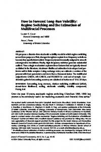
allows the introduction of the so called high density regions (HDR) (Hyndman, 1996): Rα = { X : f t l ( X ) ≥ f (α)}
(11)
where f(α) is chosen such that Pr( X t l ∈ Rα ) = 1 − α . The HDR are graphically shown in Figure 1 where the HDR are given as the union of several intervals which satisfy (11). It is clear that the region calculated using (10) masks the multimodality of f t l ( X ) implying a wider region whereas (11) is the most informative about the shape of the density. The complexity of the nonlinear models often does not allow the analytic derivation of the forecast density f t l ( X ) of the predictors. In this context the generally applicable way to obtain an approximation of the forecast density is via simulation as shown in the next section.
33
0.25 0.20 0.15 0.10 0.05 0.00
f( α )
-2
0
2
4
6
[ Q (α ) ; Q ( 1 -α )] HDR
Figure 1: Two different 100(1-α)% forecast regions for f t l (X )
4. The simulation study The forecast accuracy of the models discussed in section 2 is evaluated representing and estimating the density function of their multiperiod forecasts obtained through a Monte Carlo simulation procedure. The simulation study is implemented using three different models: AR-ARCH(2;1), SETAR-ARCH(2,1;1) and DTARCH(2,1;1,1). The selected coefficients are shown in Table 1, where the symbols used follow the notation introduced in section 2. The errors of all models are assumed Gaussian, the threshold delays of the SETAR and DTARCH models are equal to 1 and the threshold values are all fixed equal to 0. The simulated series are 1.000 for each model with length n=500, obtained after dropping the first 100 observations in order to eliminate the influence of the initialisation. For each simulated series the generation of forecasts is performed for the three models under study, at lead time l=4.
34
In order to evaluate the impact of the coefficients estimation on the forecast accuracy, the series simulated in the previous step have been used to obtain maximum likelihood estimates for the coefficients of the three models under study. This computationally intensive procedure require a fairly greater amount of computer resources due to the stability check which has been performed at each of the 1.000 iterations. Table 1: Model coefficients used in the simulation study Conditional Mean Coefficients φ10 φ11 φ12 φ02 φ12 values 0.028 -0.28 0.39 0.032 -0.45 Conditional Variance Coefficients values
α10 0.045
α11 0.13
α02 0.05
α12 0.35
The upper and lower bounds of the forecast regions (given in (10)) of the three models under study are shown in Table 2, where the empirical quantiles, at 5% and 95% confidence levels of Xˆ 500 ( 4) , are reported in case of known and estimated coefficients. Table 2: 5% and 95% empirical quantiles of the four steps ahead forecasts of the three examined models MODEL Q(0.05) Q(0.95) KNOWN COEFFICIENTS AR-ARCH -0.117 0.172 SETAR-ARCH -0.084 0.074 DTARCH -0.088 0.078 ESTIMATED COEFFICIENTS AR-ARCH -0.123 0.176 SETAR-ARCH -0.090 0.078 DTARCH -0.143 0.141 As expected, the amplitude of the interval between the 5% and the 35
95% quantile grows in presence of the estimated coefficients. The SETAR-ARCH model and DTARCH model do not show remarkable differences in the conditional mean forecast uncertainty. Their forecast variance depends non trivially upon the current information set and, as the forecast horizon increases, it will tend to converge to the unconditional variance of the process. The similar structure of the conditional mean of the SETAR-ARCH and DTARCH models implies that the shapes of the conditional mean density forecasts are not remarkably different for the two models (Amendola and Niglio, 2001). The amplitude of the forecast regions R0.05 for the SETAR-ARCH model, given as the difference between the 95% and the 5% empirical quantiles, is slightly narrower than that of the DTARCH. This suggests an increasing uncertainty of the conditional mean forecasts generated through the DTARCH model with respect to the SETAR-ARCH model. The bimodality of their forecast densities, estimated non parametrically following Silverman (1986), is evident in Figure 3 and Figure 4. In this case the forecasts are attained using the estimated coefficients which are obtained fitting the models to the simulated series generated through the conditional mean coefficients reported in Table 3. Table 3: Model coefficients for the conditional mean used in the simulation study Conditional Mean Coefficients values
φ10 φ11 -0.10 -0.28
φ12 0.39
φ02 0.20
φ12 -0.45
As expected, the predictor of the conditional mean of both models shown in Figures 3 and 4, is bimodal being the density obtained from a finite mixture distribution. Moreover, the values of their modes have suggested to better investigate on the dependence of the forecast density function upon the regime intercepts, as discussed in the next section.
36
conditional mean
0
0
1 0
2
2 0
4
3 0
6
4 0
5 0
c o n d i t i o n a l v a r i a n c e
-0.1
0.0
0.1
0.2
0.3
0.04
0.06
0.08
0.10
0.12
conditional variance
conditional mean
0
0.0
0.5
5
1.0
1.5
1 0
2.0
1 5
2.5
3.0
Figure 3: Estimated densities of the conditional mean and conditional variance of the SETAR-ARCH model
-0.2
0.0
0.2
0.4
0.6
0.00
0.05
0.10
0.15
0.20
0.25
0.30
Figure 4: Estimated densities for the conditional mean and conditional variance of the DTARCH model
5. The Effects of Parameter Estimation on Prediction Densities of DTARCH models In nonlinear time series the intercepts play an important role on the stability of the model and on the accuracy of the generated forecasts (Tong, 1995). These intercepts, which are strictly related to the initial values of 37
the data generating process, have a great impact on the shape of the density distribution and consequently on the accuracy of the forecasts generated. Franses and Van Dijk (2000) show that this impact is more evident for models characterised by a structure with regimes. In this context the relevance of DTARCH conditional mean intercepts are evaluated in order to better understand their role in forecasting. This task is performed using the simulation scheme with known coefficients described in section 4. Only the DTARCH conditional mean intercepts are differently assigned considering two different cases (Table 4): Table 4: Intercepts of the further simulated models Model 1 Model 2 φ10 = 0
φ02 = 0
φ10 = 0.10 φ02 = −0.20
whereas all the other values of the conditional mean and conditional variance are given in Table 1. The four step ahead density forecasts of the conditional mean of Model 1 and Model 2 are shown in Figure 5 and 6. Figure 5 confirms the unimodal distribution of the predictors whereas Figure 6 highlights the bimodal distribution of the forecast density which is markedly asymmetric and multimodal as the lead time increases, as shown in Amendola and Niglio (2001). The shape of the forecast density of Model 2 suggests to define the forecast region, Rα, of Xˆ 500 ( 4) , whose density is shown in Figure 6, through the high density region given in (11) which is explicitly represented through the union of two intervals: R0.10 = [-0.2712, -0.1580]∪[-0.0732, 0.1437] which are graphically shown with two grey bars.
38
0
2
4
6
8
The comparison of the shapes of the conditional mean forecast densities of Figures 5 and 6 shows the bigger uncertainty assigned to Model 2 (Figure 6) with respect to the other case and the misleading results which could be reached through the expected values E[X t+l Ψt ] , for l=4.
-0.3
-0.2
-0.1
-0.0
0.1
0.2
1
2
3
4
5
6
Figure 5: Forecast density of Xˆ t ( 4) of the DTARCH Model 1
-0.2
-0.1
0.0
0.1
Figure 6: Forecast density and HDR for Xˆ t ( 4) of the DTARCH Model 2
39
6. Concluding remarks The advantage of the forecast densities to evaluate the prediction accuracy of a selection of nonlinear time series models has been considered. The asymmetry and/or the multimodality of the predictors of some threshold conditionally heteroskedastic models have been examined through a Monte Carlo simulation study. The results obtained for the DTARCH model highlight a clear dependence of the forecast density shape on the model coefficients which has been further explored. Forecast regions and high density regions (Hyndman, 1995) have been calculated for the DTARCH model and the advantages obtained in the evaluation of the forecast accuracy are shown. The results confirm the presence of asymmetric and multimodal distribution of the predictors as the complexity of the nonlinear structure and the forecast horizon grow.
Acknowledgments : This paper is partially supported by MURST 2000 "Modelli stocastici e metodi di simulazione per l’analisi di dati dipendenti".
References Amendola A., Niglio M. (2001) Predictive distributions of nonlinear time series models, working paper n. 3.102, Dipartimento di Scienze Economiche, Università di Salerno Box G.E.P., Jenkins G.M. (1970) Time series analysis, forecasting and control, San Francisco: Holden Day Chatfield C. (1993) Calculating interval forecasts, Journal of Business & Economic Statistics, 11, 121-144 Engle R.F. (1982) Autoregressive conditional heteroscedasticity with estimates of the variance of United Kingdom inflation, Econometrica, 50, 987-1008
40
Franses P.H., Van Dijk D. (2000) Nonlinear time series models in empirical finance, Cambridge University Press: Cambridge Granger C.W., Teräsvirta T. (1993), Modelling nonlinear economic relationships, Oxford University Press, Oxford Hyndman R.J. (1995) Highest-density forecast regions for nonlinear and non-normal time series models, Journal of Forecasting, 14, 431-441 Hyndman R.J. (1996) Computing and graphing highest density regions, American Statistician, 50, 120-126 Li W.K., Lam K. (1995) Modelling asymmetry in stock returns by threshold autoregressive conditional heteroscedastic model, The Statistician, 44, 333-341 Liu J., Li W.K., Li C.W. (1997) On a threshold autoregression with conditional heteroscedastic variances, Journal of Statistical Planning and Inference, 62, 279-300 Niglio M. (2000) Previsioni per modelli non lineari di serie storiche, Tesi di Dottorato, Università di Chieti Silverman B.W. (1986) Density estimation, Chapman & Hall: London Tay A.S., Wallis K.F (2000) Density forecasting: a survey, Journal of Forecasting,19, 235-54 Tjøstheim D. (1994) Non-linear time series: a selective review, Scandinavian Journal of Statistics, 21, 97-130 Tong H. (1990) Non-linear time series: a dynamical system approach, Clarendon Press Tong H. (1995) A personal overview of nonlinear time series from chaos perspective, Scandinavian Journal of Statistics, 22, 399-445 Tong H., Lim K.S. (1980) Threshold autoregression, limit cycles and cyclical data, Journal of Royal Statistical Society (B), 42, 245-292 Weiss A.A. (1984) ARMA models with ARCH errors, Journal of Time Series Analysis, 5, 129-143
41