forecasting the ocean wave heights using linear genetic programming

Proceedings of ninth International Conference on Hydro-Science and Engineering (ICHE 2010), IIT Madras, Chennai, India. Forecasting the2Ocean Wave2010 Heights Using Linear Genetic - 5 August

Programming

FORECASTING THE OCEAN WAVE HEIGHTS USING LINEAR GENETIC PROGRAMMING Nitsure S.P.1, Londhe S.N.2 and Khare K.C.3

Abstract: Prediction of Oceanic Parameters has been a daunting task for the researchers over last few decades. In ocean engineering, wave height (usually ranging from a few centimeters to over 15m) and wave period (ranging from 1s to 30s) are two design criteria for the stability and safety of marine vessels as well as the offshore structures, subjected to wave attacks. Fairly accurate prediction of these parameters with practically useful lead time is the need of the hour. Since last couple of decades, researchers have found soft computing technique to be an efficient tool for prediction of oceanic parameters. This technique, based on inspiration from natural phenomena has the advantages and characteristics such as exact physical relationship between parameters not essential for modeling, better data error tolerance, high speed, etc. During past few years, the soft tool of Genetic Programming is being explored by few ocean researchers. Further, more efficient variants of genetic programming, such as linear genetic programming and automatic induction of machine code genetic programming are being recently tried for the prediction works. This paper presents the work on cause effect modeling (forecasting wave heights from the wind data), using linear genetic programming at two stations (which are found to get affected the worst by various hurricanes and cyclones) in the Gulf of Mexico. Keywords: Oceanic Parameters; Significant Wave Height; Forecasting; Wind Velocity Components; Soft Computing; Linear Genetic Programming. INTRODUCTION Prediction of oceanic parameters such as Significant Wave height (SWH or Hs), wave period, storm surge, etc. are very essential for all ocean related activities. Since wind is the main wave producing parameter, wind–wave relationships have been explored over a period of five decades in the past by establishing empirical equations and also by numerically solving the equations of wave growth. Different other types of wave modeling techniques (viz. Experimental/ Physical, soft computing) have also been tried out by researchers for accurate prediction of wave heights and wave periods. The high energies of the wind are transferred to the calm ocean water by the normal (perpendicular to ocean water surface) component of the wind pressure as well as by its tangential component. Consequent formation and growth of waves is influenced by factors such 1 Research Student, Department of Civil Engineering, Sinhgad College of Engineering, Pune 411 041, India, Email: [email protected] (Member, IEI, ISH) 2 Professor, Department of Civil Engineering, & Dean Academics, Vishwakarma Institute of Information Technology, Pune 411 048, India, Email: [email protected] (Member, ASCE, IAHR, IAHS, ISH, and IEI). 3 Professor, Department of Civil Engineering, & Vice Principal, Sinhgad College of Engineering, Pune 411 041, India, Email: kanchanckhare@ gmail.com (Member, ITPI, IAOH, IWRS,ISH, IEI)

1561

Forecasting the Ocean Wave Heights Using Linear Genetic Programming

as wind velocity, fetch and duration. Waves are classified as seas (the short-period waves created by the wind, very close to the area of generation) and swells (the waves that have moved out of the generating area). Long period waves move faster than short period waves, and reach distant sites first. The former lose their energy more rapidly than the latter ones. Waves of most concern to ocean engineers are generated by wind action in which the wind first creates a disturbance in the sea which is restored to its calm (equilibrium position) by the action of earth’s gravity. Hence resulting oscillatory waves are called wind generated gravity waves. Height of a wave is the vertical distance between its crest and trough (Which may vary from a few cm to over 15 m); while the period of a wave is the time required to complete one cycle of its oscillation (Which may vary from 1second to 30seconds). The horizontal spread of one wind wave (the wave length) ranges from few meters to over a kilometer. Since height of ocean wave keeps on fluctuating in general randomly, mean wave height ( ) or maximum wave height (Hmax) are usually not considered; but Significant Wave Height (denoted as Hs or H1/3 or SWH) is considered in ocean engineering studies. It is defined as the average of highest one-third of the measured wave heights. (Coastal Engineering Manual, 2008, US Army Corps of Engineering; Ministry of Commerce – United States of America) Statistical, Empirical, and Numerical Modeling methods are traditionally used for prediction of oceanic parameters. The procedures involved in these models are extremely complex and requires very large amounts of meteorological and oceanographic data. (Deo and Naidu, 1999) The physical process of generation of waves by wind is extremely complex, uncertain and not yet fully understood. (Deo et al., 2001) The complexity and uncertainty of the wave generation phenomenon is such that despite the advances in computational techniques, the solutions obtained are neither exact nor uniformly applicable at all sites and at all times. The uncertainty and randomness involved in wind wave phenomenon makes it ideally suitable for data driven (e.g. soft computing) approach which do not assume any a priori relationship between the parameters like the knowledge based approach such as analytical, numerical and empirical modeling. Since last couple of decades or so, researchers have found soft computing to be a tool better than the traditional methods for prediction of oceanic parameters. (Deo et al., 2001) During the last couple of years; the soft tool of Genetic Programming is being explored by few ocean researchers for prediction of oceanic parameters. They have found it to be still better than the previous soft tools of artificial neural network. Researchers from the field of computer software and hardware have invented special variants of genetic programming such as Linear Genetic Programming (LGP), Automatic Induction of Machine code Genetic Programming (AIM-GP), etc.; which are more efficient in evolving the desired program. For further details, readers are referred to Nordin et al. (1999), Brameier & Banzhaf (2001), and Guven (2009). This paper presents the work on forecasting of Significant Wave Height (Hs) 6hours to 24hours ahead of time at two locations in the Gulf of Mexico, using the current as well as previous values of Wind Velocity components at different elevations with respect to ocean water surface with the help of soft tool of Genetic Programming.

OVERVIEW OF LINEAR GENETIC PROGRAMMING (LGP)

1562

Forecasting the Ocean Wave Heights Using Linear Genetic Programming

Soft Computing (SC) is a collection of techniques spanning many fields that fall under various categories in Computational Intelligence and became a formal Computer Science area of study in the early nineties. Unlike hard computing systems, which strive for exactness and full truth, soft computing techniques exploit the given tolerance of imprecision, partial truth, & uncertainty for a particular problem. SC includes tools like ANN, Genetic Programming (GP), and Fuzzy Systems (FS). Solutions are not programmed by SC tools for each and every possible situation. Instead, the problem is represented in such a way that the ‘state’ of the system can somehow be measured or understood and compared with some ‘desired state’. Quality of the system’s state forms the basis for adapting and adjusting the system’s parameters, which slowly converge towards the solution. SC is often robust under noisy input environments and has high tolerance for imprecision in the data on which it operates. SC techniques are inspired from natural phenomena. viz. ANN tries to mimic human brain; GP uses the dynamics of Darwinian evolution, Fuzzy Logic is motivated by the highly imprecise nature of human speech. GP starts with a population of randomly generated computer programs on which computerized evolution process operates. Then a ‘tournament’ or competition is conducted by randomly selecting four programs from the population. GP measures how each program performs the user designated task. The two programs that perform the task best ‘win’ the tournament. GP algorithm then copies the two winner programs and transforms these copies into two new programs via crossover and mutation operators i.e. winners now have the ‘children.’ These two new child programs are then inserted into the population of programs, replacing the two loser programs from the tournament. Crossover is inspired by the exchange of genetic material occurring in sexual reproduction in biology. Tree-based Genetic Programming (TGP) and Linear Genetic Programming (LGP) are two main variations of GP. For details of GP; readers are referred to Koza (1992). LGP uses a specific linear representation of computer programs. The name ‘linear’ refers to the structure of the (imperative) program representation only, and not to the functional genetic programs that are restricted only to a linear list of nodes. On the contrary, LGP usually represents highly nonlinear solutions. Each individual (Program) in LGP is represented by a variable-length sequence of simple C language instructions, which operate on the registers (r[i]) and constants (c) from predefined sets. The function set of the system can be composed of arithmetic operations (+, –, X , / ) , conditional branches (if v[i] v[k]) etc., and the function calls (f {x, xn, sqrt, ex ,sin, cos, tan, log, ln }). LGP utilizes two-point string cross-over. A segment of random position and random length of an instruction is selected from each parents and exchanged. If one of the resulting children exceeds the maximum length, this cross-over is abandoned and restarted by exchanging equalized segments. LGP also employs a special kind of mutation, called as ‘macro mutation’, which deletes/ inserts an entire instruction. The readers are referred to Brameier and Banzhaf (2001) for further details. Main characteristics and advantages of LGP over TGP can be stated (Guven, 2009) as: (1)Each individual program in LGP is represented by a variable–length sequence of simple C language instructions. (2)Generation of efficient code by removal of non–effective instructions/ introns (3)The instructions operate on one or more registers and/or the constants from predefined data sets. (4)The expressions of a functional programming language (like LISP) are substituted by programs of an imperative language such as C or C++. (5)The graph based data flow and evolving programs in a low-level language; in which solutions are directly manipulated as binary

1563

Forecasting the Ocean Wave Heights Using Linear Genetic Programming

machine codes; executed without using an interpreter, result into faster evolution of programs. Automatic Induction of Machine code by Genetic Programming (AIM-GP) is further a special variant of LGP. In AIM-GP, individuals are manipulated as binary machine code in the memory and are executed directly without passing an interpreter during the fitness calculation resulting into a significant speedup compared to interpreting systems. Instruction Blocks in the body of the program may contain one or more instructions with functions such as SIN, COS, POW, ABS, SQRT, LN, EXP, etc. and/or arithmetical operators such as +, –, *, /, etc. Mainly two point block homologous crossover operator (i.e. Instruction Block or Blocks are swapped between the parent programs) is used in AIM-GP. However, some non-homologous (i.e. ordinary) crossover is necessary to change the length of genomes. Crossover occurs only at the boundaries of the IB and without reference to the contents of the IB. (Nordin et al., 1999). Mutation operator makes random changes in randomly chosen instruction to a randomly chosen block. Thus, an evolved LGP program is a sequence of binary machine instructions. For example, an evolved program might be comprised of a sequence of four, 32-bit machine instructions. When executed, those four instructions would cause the Central Processing Unit (CPU) to perform operations on the CPU’s hardware registers. An example of a simple, fourinstruction LGP that uses three hardware registers is given below: register 2 = register 1 + register 2 register 3 = register 1 - 64 register 3 = register 2 * register 3 register 3 = register 2 / register 3 Commercial Software Discipulus, based on AIM-GP used for this work writes a computer program to model the data. It assembles ‘Program’ and ‘Team’ Models during each ‘Project’. Program Model is a single program written by Discipulus to model the data and combines single program models to give a Team Model that would give better results than a single individual program model. It creates total 30 programs in a project and produces total five teams of 1, 3, 5, 7 and 9 program combinations. APPLICATION OF GP FOR WAVE MODELING Use of GP for modeling waves is very recent and only a handful of papers are available in the literature. Charhate et al. (2007) used GP for spatial mapping of storm surge, tsunami water levels, and currents. Kalra and Deo (2009), and Ustoorikar and Deo (2008), used GP for filling the gaps in the measured wave data. Online wave forecast for 3, 6, 12, and 24 hours lead time is tried by Gaur and Deo (2008) using GP. They found that prediction for longer lead times (12 and 24 hours) and for higher SWH values were less accurate. Jain and Deo (2008) used data driven tools of ANN, GP and Model Tree (MT) for real time wave forecasting and recognized that 72h lead time forecasting accuracies were possible with target waves less than 6m and 2.5m for offshore and coastal locations respectively. Kalra et al. (2008) used GP for projecting coastal deep water wave heights. They noticed that GP performed excellently over most of the levels of wave heights. Londhe (2008) used GP to correlate wave measuring locations and found it suitable in extreme events like hurricanes as well. Kambekar and Deo (2010, in press), used sequence of past 24 hourly measurements of wind speed and wind direction to predict Hs and average wave period (Tz) 24hours ahead of time with the help of soft tools of GP and MT.

1564

Forecasting the Ocean Wave Heights Using Linear Genetic Programming

Present work is an attempt to predict the significant wave height by using current and previous N-S and E-W components of the wind velocities Uz, U10, and U* with the soft tool of GP. STUDY AREA AND DATA Present study is done at two Stations owned and maintained by National Data Buoy Centre (NDBC) of National Oceanic and Atmospheric Administration (NOAA) of the United States of America: Station 42007 (at 300 5’ 25” N, 880 46’ 7” W, and 22 nautical miles South-Southeast of Biloxi) and Station 42040 (Mobile South, having location 290 12’ 19” N, 880 12’ 19” W, and 64 nautical miles South of Dauphin island, Alabama) Fig.1 shows their locations. In this region, the season of Hurricanes is from May to November. 27 hurricanes have hit this area in the year 2005 and 17 have hit in 2008 as shown in Fig.2. (Reference: Atlantic Hurricane tracks on www.nhc.noaa.gov/2008atlan.shtml)

Fig. 1. Locations of the Wave Rider Buoy Stations. Fig. 2.

Hurricanes in the Gulf of Mexico in the year 2008.

Water depths at these locations are 14.9m and 274.3m respectively. The wind velocity, wind direction and significant wave height data observed at these locations for five years of 2002 to 2005 is used to calibrate and test the separate models at station 42007 and 42040 with data sorted

1565

Forecasting the Ocean Wave Heights Using Linear Genetic Programming

with time steps of 1h, 3h, 6h, and 12h. Instead of using wind direction in degree units the wind velocity is decomposed into cosine and sine components using the particular wind velocity Uz (at the anemometer elevation of 5m) or U10 (at universally accepted elevation of 10m) or U* (shear or friction velocity) and the measured wind direction (U10 and U* at each station were calculated at the present time‘t’ from the hourly data of wind speed, wind direction, and Hs). The wind velocity components at time ‘t’ and at previous times with time steps of 1hour, 3hours, and 6hours were arranged as inputs and values of Hs with lead times of 6hours, 12hours, 18 hours, and 24hours were arranged as output for various trials. (Total number of data sets used is 4920 at this station). It was found that a time step of 6 hours produced better results than other time steps for forecasting of Hs. It is also noticed that results with very large data of 4 or 6 years (at station 42007) has no effect on the accuracy of the results. Based on these results, and to include the extreme Hs values in modeling, data of years 2004 and 2005 was only used for the model at station 42040. (Total 2532 data sets used for this model).

MODEL DEVELOPMENT Present work involves use of current and previous values of wind velocities to forecast the current wave height at two wave rider buoy stations. Steps followed for the forecasting work are: (1) Wave Buoy Data (hourly values of Hs, wind speed and wind direction from January 2004 to December 2008) was downloaded from the web-site. (2) Wind Velocity components (WV x cos and WV x sin ) at three different elevations were computed for all values of observed wind speed U and wind direction . viz. components of the wind velocity (i)Uz at the anemometer level ‘z’, (ii)U10 at the universally accepted 10m elevation, and (iii)shear velocity U*. Velocities U10 and U* were found out using (standard) equations 1 and 2 given below. 10 U10 = (Uz). z

1 7

(1)

and U* = U10 C D

(2)

Value of wind drag coefficient CD are obtained by equation 3 and 4 given below (Wu, 1982) CD =1.2875x10–3 for U10 < 7.5 m/s (3) CD = (0.8 + 0.065 x U10) x10–3 for U10 >7.5 m/s

(4)

(3) 70% of the total data was used for training and 30% was kept aside for testing (validation). (4) Components of WV (Wind Velocity, which is either Uz, or U10, or U*) at the present (current) time ‘t’, and previous times ‘t–6’, ‘t–12’, ‘t–18’, and ‘t–24’ were arranged as inputs. Hs at time‘t + C’ as output for final forecasting model. Trials with lead times C = 6, 12, 18, and 24 were conducted successively. Thus the functional relationship is given by equation 5. (Hs)t+C = f {[(WV). cosine( )(t, t–C, t–2C, t–3C, t–4C)] , [(WV).sine( )(t, t–C, t–2C, t–3C, t–4C)]}

(5)

(5) Initial GP Parameters selection: Population size 500; Program size: initial 80, maximum 512; randomized constants (their values are between –1 to +1); Cross-over frequency 50% ,

1566

Forecasting the Ocean Wave Heights Using Linear Genetic Programming

Homologous cross over 95%, Mutation frequency 95%, block and instruction mutation rates 30% each, instruction data mutation 40%; and instruction set: addition, arithmetic, comparison, exponential, multiplication, subtraction, trigonometric. (6) Trial was terminated at the when performance of program and team was seen to be saturated. (7) The project was saved and result parameters (fitness, correlation coefficient ‘r’) for that trial were recorded for the best program and for the best team. The fitness function was Mean Squared Error (MSE). (8) Calibrated model was then applied to an unseen data set. The error measures were monitored on this data set and the models were finalized when very low value of error was achieved. (MSE was used at this stage as error measure to assess the performance of the model) (9) Another error measure Root Mean Squared Error (RMSE) was also used to assess the performance of the model. Equations 6 through 8 give the formulae for the error measures and for correlation coefficient ‘r’. 1 n

MSE

RMSE

n

2

(6)

i 1

MSE

n i 1

r

Hˆ i

Hi

Hi

n

Hi

H

(7)

H 2

Hˆ i n i 1

Hˆ i

~ H

(8) ~ H

2

i 1

Where Hi = target (observed) wave height Hˆ = output wave height i

H = mean of the target wave heights ~ H = mean of output wave heights n = total number of target and output pairs RESULTS AND DISCUSSION In general, results with shear wind velocity seem to be better than those with other wind velocity components, as can be expected because the tangential component of wind velocity on the water surface is the prime cause of waves. There is not much difference between the results with Uz, and U10 components. This is due to negligible variation in the wind profile at 5m and 10m elevations. Results at the station in open wider area and deep water location is better than that at the shallow water location near the coast. This may be due to space and time averaging effect on the data used. The Best Team results with the time step of 6hours for three types of wind velocity components, as mentioned in ‘model development’, are shown in table 1 and table 2.

1567

Forecasting the Ocean Wave Heights Using Linear Genetic Programming

Table 1. Fitness and Correlation Coefficient ‘r’ (station 42007) Lead Time Results with Uz Results with U10 Results with U* 6hours

0.08, 0.76

0.08, 0.76

0.14, 0.81

12hours

0.10, 0.70

0.09, 0.71

0.17, 0.72

18hours

0.10, 0.66

0.10, 0.67

0.20, 0.64

24hours

0.11, 0.63

0.11, 0.63

0..23, 0.57

Table 2. Fitness and Correlation Coefficient ‘r’ (station 42040) Lead Time Results with Uz Results with U10 Results with U* 6hours

0.16, 0.95

0.19, 0.94

0.18, 0.95

12hours

0.32, 0.91

0.29, 0.91

0.31, 0.91

18hours

0.55, 0.83

0.50, 0.85

0.43, 0.84

24hours

0.79, 0.72

0.68, 0.80

0.80, 0.75

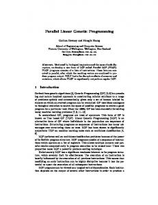
Scatter plots between observed and predicted Hs at station 42040 with components of Uz as inputs up to previous 24h are shown in fig. 3; which indicate that forecast is fairly satisfactory.

r = 0.93

r = 0.95

Fig. 4. Scatter Plots (station 42040) for 6hourly Uz components up to past 24hours The results with the time step of 6h were better than the other time steps perhaps because the underlying physics was understood the best by genetic programming through these data sets. The evolved models suggest that there is an effect of about past day’s wind velocities on the wave heights measured at a station. It is also seen that data of many years has not been beneficial for forecasting the waves. Wind velocity components (cause) of a couple of years which include the peaks is sufficient for GP to understand their effect-the waves. Plots of Hs and peaks at station

1568

Forecasting the Ocean Wave Heights Using Linear Genetic Programming

42040 with 6hourly data and components of Uz up to previous 24h are shown in fig. 4 and 5

Fig. 4. Wave Plot (Station 42040) for 6hourly Uz components up to past 24hours

Fig. 5. Plot of Peak Hs (Station 42040) for 6hourly Uz components up to past 24hours

CONCLUSIONS Results with shear velocity components are better than the other types of velocity components and accuracy of forecast is found to decrease with increase in lead time. It is seen that wind-wave mapping at the station in open wider area and deep water location is better than that at the shallow water location near the coast. Wave height forecasts using the wind velocity components and GP tool at two locations in the Gulf of Mexico, USA is done satisfactorily. Splitting wind velocity in its components seems to have worked well, as shown by the scatter plots and error measures. All models forecasted the peak wave heights with reasonable accuracy with marginal or no phase shift, making it useful throughout the year. The technique of GP for wave forecasting with wind velocity components as input needs to be studied and explored further to improve the accuracy of prediction with higher lead times and at peak values at different locations.

1569

Forecasting the Ocean Wave Heights Using Linear Genetic Programming

REFERENCES Brameier M., Banzhaf W. 2001. Evolving teams of predictors with linear genetic programming. Genetic Programming and Evolvable Machines, vol. 2(4), 381–407 Charhate, S.B., Deo, M.C. 2007. Application of genetic programming to coastal and ocean problems. Int Workshop on Advances in Hydroinformatics, Niagara Falls. Charhate S.B., Deo M.C., Sanil Kumar V. 2007. Soft and Hard Computing Approaches for Real Time Prediction of Coastal Currents in a Tide Dominated Area. J Engineering for the Maritime Environment, Vol. 221(4)(2007), 147-163 Coastal Engineering Manual, US Army Corps of Engineering; Ministry of Commerce – United States of America (2008) Deo M. C., Naidu C. S. 1999. Real time wave forecasting using neural networks. Ocean Engineering, 26 (1999), 191-203. Deo M. C., Jha A., Chaphekar A.S.,Ravikant K. 2001. Neural networks for wave forecasting. Ocean Engineering, 28 (2001), 889-898. Gaur S., Deo M. C. 2008. Real time wave forecasting using genetic programming. Ocean Engineering, 35 (2008), 1166-1172 . Guven A. 2009.Linear Genetic Programming for time series modelling of daily flow rate. J Earth System Sciences, 118, No.2, April 2009, 137-146. Jain P., Deo M. C. 2008. A.I. tools to forecast ocean waves in real time. The Open Ocean Engineering Journal, 1(2008), 13-21. Kalra, R., Deo, M. C., Raj Kumar, Agarwal, V. K. 2008. Genetic programming to estimate coastal waves from deep water measurements. Int J Ecology and Development, Indian Society for Development and Environment Research Roorkee, India, ISSN 0972-9984, 10, S08, 6776. Kalra R., Deo M. C. 2009. Genetic programming to retrive missing information in wave records along the west coast of India. Applied Ocean Research, 29(2009), 99-111. Kambekar A.R., Deo M.C. 2010. Wave simulation and forecasting using wind time history and data driven methods. Int J Ships and Offshore Structures, Taylor and Francis, TSOS 444283 Koza J.R. 1992. Genetic Programming: On the programming of Computers by means of natural selection. A Bradford Book, MIT Press. Londhe S.N. 2008. Soft computing approach for real-time estimation of missing wave heights. Ocean Engineering, 35 (2008), 1080-1089. Nordin P., Hoffmann F., Francone F., Brameier M., Banzhaf W. 1999. AIM-GP and parallelism. Proc Congress on Evolutionary Computation (CEC ’99), IEEE Press, Piscataway, NJ, 1059–1066. Ustoorikar K., Deo M. C. 2008. Filling up the gaps in wave data with genetic programming. Marine Structures, Elsevier, 21(2-3) (2008), 177-195. Wu, J. 1982. Wind stress coefficients over sea surface from breeze to hurricane. J Geophysical Research, 87 (C12), 9704–9706.

1570