Page 1 of 7
1 2 3 4 5 6 7 8 9 10 11 12 13 14 15 16 17 18 19 20 21 22 23 24 25 26 27 28 29 30 31 32 33 34 35 36 37 38 39 40 41 42 43 44 45 46 47 48 49 50 51 52 53 54 55 56 57 58 59 60
Form-finding of grid shells with continuous elastic rods Jian-Min Li PhD student Institute of Building Structures and Structural Design (itke), University Stuttgart Stuttgar, Germany
Jan Knippers Prof. Dr.-Ing. Institute of Building Structure and Structural Design (itke), University Stuttgart Stuttgart, Germany
[email protected]
[email protected]
Keywords: grid shells; form-finding; elasticity; free-form; dynamic relaxation; NURBS; least strain energy; constraints; mapping; residual forces.
Abstract Grid shells with continuous elastic rods have the advantages to generate curved spaces with uniform members and joints. The joints connecting the crossing rods are capable of in-plane rotation. This makes grids lack the in–plane rigidity and allows grids to take large deformations during erection/formation process. Besides, members in these elastic structures are in bended states, thus when they are all combined together they can easily generate single or double curved space. This character makes elastic grid shell have the potential to be the structures of free-form architectures. However, finding the boundary conditions, including the grid pattern and bearing positions, which lead to a specific geometry, is not an easy task. Designers have to keep equal grid lengths, minimise the residual forces, ensure the smoothness and attain the desired geometry simultaneously. In short of an appropriate numerical method, designers of the projects like Mannheim Multihall and Downland Museum returned to physical models to find the boundary conditions. The complicated and multi-steps form-finding process makes this kind of structure less popular to architects/engineers and only a few building projects were realized. This paper describes a new numerical method which can derive the grid pattern and bearing positions according to a desired geometry. This is done by finding the least strain energy state of the elastic grid in the solution domain defined by constraints. This method can provide architects a grid pattern that satisfies all the geometrical demands. At the same time, a result with least strain energy is favoured by engineers. This is especially important for an elastic grid shell, whose structural stability is largely affected by the residual forces. The rest of the paper is organized as follows. In section2, we discuss related works and give our iterN = 10 iterN = 1 assessment to each method. Section 3 gives a detailed description of the theorem that our method is based on. A physical model is used to help readers to build a general idea of our method. Then, more detailed description of our numerical method is presented. A grid shell with the shape of Downland museum is generated by our method as illustration (Fig.1). In section 4, we discuss the deformations of elastic grid shells, caused by residual forces, by analyzing the iterN = 100 iterN = 1000 illustrative example in section 3. Finally, a Fig. 1: stages of iteration conclusion is given.
Page 2 of 7
1 2 3 4 5 6 7 8 9 10 11 12 13 14 15 16 17 18 19 20 21 22 23 24 25 26 27 28 29 30 31 32 33 34 35 36 37 38 39 40 41 42 43 44 45 46 47 48 49 50 51 52 53 54 55 56 57 58 59 60
Form-finding of grid shells with continuous elastic rods Jian-Min Li PhD student Institute of Building Structures and Structural Design (itke), University Stuttgart Stuttgar, Germany
Jan Knippers Prof. Dr.-Ing. Institute of Building Structure and Structural Design (itke), University Stuttgart Stuttgart, Germany
[email protected]
[email protected]
Summary Grid shells with continuous elastic rods have the advantages to generate curved spaces with uniform members and joints. However, finding the boundary conditions, including the grid pattern and bearing positions, which lead to a specific geometry, is not an easy task. Designers have to keep equal grid lengths, minimise the residual forces and ensure the smoothness of geometries simultaneously. In this paper, we present a new numerical method which can derive the grid pattern and bearing positions in accordance with a desired geometry. This is done by finding the least strain energy state of the elastic grid in the solution domain defined by constraints. This method can provide architects a grid pattern that satisfies all the geometrical demands. At the same time, a structure with less strain energy is favoured by engineers. This is especially important for elastic grid shells, whose structural stability is largely affected by the residual forces. Keywords: grid shells; form-finding; elasticity; free-form; dynamic relaxation; NURBS; least strain energy; constraints; mapping; residual forces.
1.
Introduction
Grid shells with continuous elastic rods have the advantages to generate curved spaces with uniform members and joints. The joints connecting the crossing rods are capable of in-plane rotation. This makes grids lack the in–plane rigidity and allows grids to take large deformations during erection/formation process. Besides, members in these elastic structures are in bended states, thus when they are all combined together they can easily generate single or double curved space. This character makes elastic grid shell have the potential to be the structures of free-form architectures. However, finding the boundary conditions, including the grid pattern and bearing positions, which lead to a specific geometry, is not an easy task. Designers have to keep equal grid lengths, minimise the residual forces, ensure the smoothness and attain the desired geometry simultaneously. In short of an appropriate numerical method, designers of the projects like Mannheim Multihall and Downland Museum returned to physical models to find the boundary conditions. The complicated and multi-steps form-finding process makes this kind of structure less popular to architects/engineers and only a few building projects were realized. This paper describes a new numerical method which can derive the grid pattern and bearing positions according to a desired geometry. This is done by finding the least strain energy state of the elastic grid in the solution domain defined by constraints. This method can provide architects a grid pattern that satisfies all the geometrical demands. At the same time, a result with least strain energy is favoured by engineers. This is especially important for an elastic grid shell, whose structural stability is largely affected by the residual forces. The rest of the paper is organized as follows. In section2, we discuss related works and give our assessment to each method. Section 3 gives a detailed description of the theorem that our method is based on. A physical model is used to help readers to build a general idea of our method. Then, more detailed description of our numerical method is presented. A grid shell with the shape of
Page 3 of 7
1 2 3 4 5 6 7 8 9 10 11 12 13 14 15 16 17 18 19 20 21 22 23 24 25 26 27 28 29 30 31 32 33 34 35 36 37 38 39 40 41 42 43 44 45 46 47 48 49 50 51 52 53 54 55 56 57 58 59 60
Downland museum is generated by our method as illustration. In section 4, we discuss the deformations of elastic grid shells, caused by residual forces, by analyzing the illustrative example in section 3. Finally, a conclusion is given.
2.
Related works and our assessment
Hanging chains models can generate funicular geometries that have only tension forces while taking gravity load. Inverting the geometries of funicular, designers can get ideal shell geometries that have only compression forces when taking gravity load. The idea was first introduced by the physician Hook in the 17th century, further developed by the architect Gaudi in the 18th [1], and applied in the form-findings of grid shells by Frei Otto in 1970s[2]. The geometries derived in this way have good performance while taking gravity load, however when lateral or uneven loading is dominant, this method loses its advantages. Besides, gravity loads takes the main role in the formations of hanging chains models. This will limit possible geometries of grid shells. The method of the Chebyshev net, also known as the compass method, is a geometrical method. The drawing of the Chebyshev net starts from two arbitrary intersecting curves on a surface. Each curve is composed of segments with the same mesh width. The rest nodal points are only determined by finding intersection from two adjacent nodes with the same mesh width (Fig.1). The method was first Fig. 1: the Chebyshev net / the compass method, IL(2) seen in the work of P.L. Chebyshev in 1878 [3] and further researched by Frei Otto in 1970s. It has the advantage to adapt to free form surfaces. But it does not take account of bending behaviours of elastic materials. Elastic grid shells with the geometries derived in this way are not in static equilibrium and may transform to other shapes. This will bring additional stresses in members and extra difficulties for erection. Chris William and M.R. Barnes developed a way using dynamic relaxation method to compute the mechanics of elastic rods [4]. Chris William applied the method to build the numerical model of Downland Museum (Fig.2) [5]. In that case, physical models were still used to decide the boundary conditions [6]. The team of Institut Navier also applied this method to design a grid shell in composite material [7]. The form-finding in that case started from a specific cutting pattern and stopped while an aesthetic shape is formed during the upwards pushing process. The relationship between the boundary conditions and the correspondingly Fig. 2: Downland museum, designed by Edward generated form remains unclear. Cullinan, engineered by Buro Happold, Singleton England, 2002, The team of Institut Navier also proposed a (www.photoblog.com/girafferacing/2009/08/16/) way of mapping continuous elastic grids on given surfaces [8]. The dynamic explicit finite element analysis was used to simulate plane elastic grids laid on imposed surfaces under the traction of gravity. This method is able to create a grid shell structure complying with specific surfaces while taking bending behaviours into consideration. However, the traction by gravity will further twist grid geometries and lead geometries to follow the direction of gravity. This phenomenon will limit possible geometries and bring additional stresses in elastic rods. The traction by gravity could be seen as an additional constraint in our method by taking it as extra nodal loads during the form-finding process.
Page 4 of 7
1 2 3 4 5 6 7 8 9 10 11 12 13 14 15 16 17 18 19 20 21 22 23 24 25 26 27 28 29 30 31 32 33 34 35 36 37 38 39 40 41 42 43 44 45 46 47 48 49 50 51 52 53 54 55 56 57 58 59 60
3.
Mapping grids by finding the minimal strain energy state
Our method is based on the phenomenon that if a grid composed of continuous elastic rods is constrained on a surface, it shall transform into a specific geometry with the minimal strain energy. This is the key point of our mapping method. In the following text, a physical model is used to help readers to build a general idea of our method. Then, more detailed description of our numerical method is presented. A grid shell with the shape of Downland museum is generated by our method as illustration.
3.1
Physical model
The mechanism of least strain energy can be more easily understood by the physical model as in Fig.3. The grid is composed of 20 continuous elastic rods. The joints between the crossing rods are designed to allow in-plane rotation. The chair back surface and the points fixed by the hand are taken as constraints. It shows that with only a few nodes constrained on the surface the rest nodes will fit into the surface by the mechanism Fig. 3 : physical model of elasticity. If we fix the nodes in other positions, the grid will automatically adjust its whole shape and form another smooth geometry immediately. After fixing the boundaries and removing the mould (the chair in Fig. 3) the geometry of the grid will change slightly until an equilibrium state is reached. 3.2 Numerical model We divide the process of building numerical model into two stages. First, we use dynamic relaxation method to build a model which can simulate the mechanism of elastic rods. Second, we derive the geometrical information from NURBS and apply it as surface and curve constraints to the model. 3.2.1 Simulating mechanism by dynamic relaxation method Using the method of dynamic relaxation (DR), we can transform the elastic rod system into a particle system [9]. The axial forces and bending momentums in rods can be calculated from the distances between particles and the included angles defined by lines which connect particles [7]. We can derive the velocities and positions of particles in the next time step by values already known in the previous time step. Therefore, we can get the dynamic of the system in time history. Furthermore, we apply kinetic damping [9] into the dynamic system such that the system will gradually run out of its kinetic energy and finally reach a static equilibrium state. 3.2.2 Applying constraints We apply constraints by confining the particles always moving on the constraint surfaces and curves. It is done by projecting each particle to the nearest point on the constraint surface/curve in each iteration circle as well as modifying each particle’s velocity as in (1) that only the tangential part is active. The unit vector nˆi is normal to the assigned surface/curve at the position of node i . v v v Vi tan = Vi − (Vi ⋅ nˆ i ) nˆ i
(1)
We can detect if the equilibrium state is reached by checking the tangential part of the net force is smaller than a given value for every particle.
Page 5 of 7
1 2 3 4 5 6 7 8 9 10 11 12 13 14 15 16 17 18 19 20 21 22 23 24 25 26 27 28 29 30 31 32 33 34 35 36 37 38 39 40 41 42 43 44 45 46 47 48 49 50 51 52 53 54 55 56 57 58 59 60
3.3
Example
initial square grid nodes on longer sides curve constraint
surface constraint
Fig. 4: elastic grid and constraints (surface with span 15.7m, height 9.5m; mesh length 1m)
iterN = 1
iterN = 100
iterN = 10
We further illustrate our numerical method by generating a grid shell with the geometry of Downland Museum. One important characteristic of this “triple-bulb double hourglass” grid shell is that it is generated from a square grid [5]. After the formation, the nodes on the longer sides of the initial square grid are resituated on the curved building foundation. The shell’s boundary condition can not be found by the existing numerical form-finding methods as described in section 2. Physical models were used by the design team to find the positions and the tilting angles of bearing points [6]. Below we show how we solve this difficulty with our new method. The initial square grid is composed of 104 crossing elastic rods with profile 5x5cm in wood with E modulus 104 N/mm2 (Fig.4). The nodes on the longer sides are constrained to move along the edge curves while the rest nodes are constrained to move on the surface. Fig.5 shows that the grid goes through different stages and reaches the final equilibrium state with a smooth grid configuration with equal grid lengths. Initial length of grid members is 1 m. The lengths after mapping are changed due to the axial forces in members. The longest member is 0.21mm longer than initial length and the shortest member is 0.25mm shorter than the initial length.
iterN = 1000
Fig. 5: stages of iteration
4.
Geometries of bearing structures
Maintaining shape is the basic issue for elastic grid shells. One crucial question arises here. Once the constraints are removed, will the grid structure stay in place and keep its geometry? In order to answer this, we need to transform our mapping results into real bearing structures. We can make it by replacing previous constraints by real bearing conditions, adding optional bracings, and adding edge beams if there are open ends. After that, we need to relax the structure once again to get a shell geometry which is in balance with residual forces. 4.1 The deformation by residual forces In order to answer the above-mentioned question, we transform the grid pattern derived in 3.3 to a bearing structure and observe its deformations by residual forces. We remove the surface and curve constraints and assign bearing points as hinge. Edge beams are added to the two open ends. Each edge beam is composed of 4 coupled elastic rods with profile 5x5cm in wood (Fig.6).
edge beam
bearing points
Fig. 6: bearing structure
Page 6 of 7
1 2 3 4 5 6 7 8 9 10 11 12 13 14 15 16 17 18 19 20 21 22 23 24 25 26 27 28 29 30 31 32 33 34 35 36 37 38 39 40 41 42 43 44 45 46 47 48 49 50 51 52 53 54 55 56 57 58 59 60
The deformations after the surface is removed are shown in Table 1. The largest deformation is on the top of the edge beam, with magnitude 90cm, which is mainly caused by the elasticity in edge beams. The second largest deformation occurs on the shell’s waist area, which is in the section C (Fig.7), with magnitude 59cm. Then, we try another bearing condition by changing the bearing points as fixed joints such that the positions and tilting angles are fixed. The largest deformation occurs still on the tops of the edge beams, with Fig. 7: plane view and section axes magnitude 90cm, 1/10 compared with the height of the structure. The second largest deformation occurs in waist areas, with magnitude 49cm. These variations from the constraint geometry are acceptable for us, since the structure still maintains its characteristic geometry and smooth pattern. We made another test by adding bracings as in Downland museum and using hinges instead of fixed joints for bearing points. The result shows that the deformation on the tops of the edge beams shrinks dramatically to 9cm. The elastic shell matches the constraint surface very well. A
B
C
D
Table 1: deformations under different conditions deformation
Perspective
Side view
Section A
Section B
Section C
Section D
Hinge bearings
Fixed bearings
Hinge bearings with bracings
Page 7 of 7
1 2 3 4 5 6 7 8 9 10 11 12 13 14 15 16 17 18 19 20 21 22 23 24 25 26 27 28 29 30 31 32 33 34 35 36 37 38 39 40 41 42 43 44 45 46 47 48 49 50 51 52 53 54 55 56 57 58 59 60
5.
Conclusion
We propose a new numerical method which can derive the grid pattern and bearing positions in accordance with a desired geometry. This is done by finding the least strain energy state of the elastic grid in the solution domain defined by constraints. This method can provide architects a grid pattern that satisfies all the geometrical constraints. At the mean time, a result with least strain energy is favoured by engineers. This is especially important for an elastic grid shell, whose structural stability is largely affected by the residual forces. We further show the feasibility of this method by generating a grid shell with the geometry of Downland museum.
References [1]
Graefe R., “On the form development of archs and vaults (in German)”, Journal of History of Architecture, Munchen-Berlin, 1986, pp. 50-67
[2] [3]
IL 10, “IL 19 Grid Shells”, Institute for the Lightweight Structures, 1974, Stuttgart. Eugene Vladimirovich Popov, “Geometri Approach to Chebyshev Net Generation Along an Arbitrary Surface Represented By NURBS”, International Conference Graphicon 2002, Nizhny Novgorod, Russia S. Adriaenssens, M.R. Barnes, and C.J.K. Williams, “A new Analytic and Numerical basis for the Form-finding and Analysis of Spline and Grid-shell”, Computing Developments in Civil and Structural Engineering, 1999, pp. 83-90 Ollie Kelly, Richard Harris, Michael Dickson, and James Rowe, “Construction of the Downland grid shell”, Structural Engineer, 79:1717, 2001, pp. 25-33. Rowe, J. and Harris, R. “The structural engineering of the Downland Gridshell”, IABSE Conference: Innovative Wooden Structures and Bridges, 2001, pp. 29-31 August, Lahti, Finland. C. Douthe, O. Baverel, J.-F. Caron, “Form-finding of a grid shell in composite materials”, Journal of IASS, 2006. Lina BOUHAYA, Olivier BAVEREL, Jean-François CARON , “Mapping two-way continuous elastic grid on an imposed surface”, Proceedings of the IASS Symposium, 2009, pp. 989-997,Valencia. M.R. Barnes, “Form finding and analysis of tension structures by dynamic relaxation”, International Journal of Space Structures, Vol. 14 No. 2, 1999, pp. 89-104.
[4]
[5] [6]
[7] [8]
[9]