Formal aspects of component software

Formal aspects of component software M. Sun, B. Schatz SEN-E0902

Centrum Wiskunde & Informatica

Centrum Wiskunde & Informatica (CWI) is the national research institute for Mathematics and Computer Science. It is sponsored by the Netherlands Organisation for Scientific Research (NWO). CWI is a founding member of ERCIM, the European Research Consortium for Informatics and Mathematics. CWI's research has a theme-oriented structure and is grouped into four clusters. Listed below are the names of the clusters and in parentheses their acronyms. Probability, Networks and Algorithms (PNA) Software Engineering (SEN) Modelling, Analysis and Simulation (MAS) Information Systems (INS)

Copyright © 2009, Centrum Wiskunde & Informatica P.O. Box 94079, 1090 GB Amsterdam (NL) Science Park 123, 1098 XG Amsterdam (NL) Telephone +31 20 592 9333 Telefax +31 20 592 4199 ISSN 1386-369X

Sun Meng & Bernhard Schätz (Eds.)

Formal Aspects of Component Software

6th International Workshop, FACS 2009 Eindhoven, the Netherlands 2-3 November, 2009 Pre-Proceedings

Formal aspects of component software ABSTRACT This is the pre-proceedings of 6th International Workshop on Formal Aspects of Component Software (FACS'09). 2000 Mathematics Subject Classification: 00 1998 ACM Computing Classification System: A.0 Keywords and Phrases: Proceedings

Preface This volume contains the proceedings of the 6th International Workshop on Formal Aspects of Component Software (FACS09). FACS’09 was held in Eindhoven, the Netherlands on November 2-3, 2009 as a satellite event of the Formal Methods Week. The objective of FACS’09 is to bring together researchers in the areas of component software and formal methods to promote a deep understanding of this paradigm and its applications. Componentbased software has emerged as a promising paradigm to deal with the ever increasing need for mastering systems’ complexity, for enabling evolution and reuse, and for bringing sound production and engineering standards into software engineering. However, many issues in component-based software development remain open and pose challenging research questions. Formal methods consist of mathematically-based techniques for the specification, development and verification of software and hardware systems. They have shown their great utility for setting up the formal foundations of component software and working out challenging issues such as mathematical models for components, their composition and adaptation, or rigorous approaches to verification, deployment, testing and certification. FACS’09 is the 6th event in a series of workshops, founded by the International Institute for Software Technology of the United Nations University (UNU-IIST). The first FACS workshop was co-located with FM’03 (Pisa, Italy, September 2003). The following FACS workshops were organised as standalone events, respectively at UNU-IIST in Macau (October 2005), at Charles University in Prague (September 2006), at INRIA in Sophia-Antipolis (September 2007), and at University of Málaga in Spain (September 2008). FACS’09 was scheduled as part of the first Formal Methods Week (FMweek), to be hosted by Technische Universiteit Eindhoven in Eindhoven, the Netherlands, in November 2009. The scientific program includes 13 regular papers and 2 invited talks, delivered by Gert Döhmen from AIRBUS Deutschland GmbH, Hamburg, Germany and by Jan Rutten from CWI, Amsterdam, the Netherlands. Each paper was reviewed by at least three Program Committee members. The entire reviewing process was supported by the EasyChair Conference System. We would like to express our gratitude to all the researchers who submitted their work to the workshop and to all colleagues who served on the Program Committee and helped us in preparing a high-quality workshop program. We are also most grateful to the invited speakers for the willingness to present their research and to share their own perspectives on formal methods for component software at the workshop. Without the support of TU Eindhoven, CWI and UNU-IIST this workshop could not have happened. We are most grateful to all organizing institutions and staff for supporting FACS and providing an organizational framework for the workshop. In particular, we are deeply indebted to Erik de Vink and Tijn Borghuis at TU Eindhoven, Jos van der Werf and Jan Schipper at CWI, and Kitty Chan Iok Sam at UNU-IIST Macau, for their help in managing the practical aspects of this event. Sun Meng and Bernhard Sch¨ atz FACS’09 PC Chairs

Organization

Steering Committee Zhiming Liu (IIST UNU, Macau, China, coordinator) Farhad Arbab (CWI, The Netherlands) Luis Barbosa (Universidade do Minho, Portugal) Carlos Canal (University of Málaga, Spain) Markus Lumpe (Swinburne University of Technology, Australia) Eric Madelaine (INRIA, Sophia-Antipolis, France) Vladimir Mencl (Charles University, Prague, Czech Republic, and University of Canterbury, New Zealand) Corina Pasareanu (NASA Ames Research Center, USA) Sun Meng (CWI, the Netherlands) Bernhard Schätz (Technical University of Munich, Germany)

Programme Chairs Sun Meng (CWI, the Netherlands) Bernhard Schätz (Technical University of Munich, Germany)

Programme Committee Farhad Arbab (CWI, The Netherlands) Luis Barbosa (Universidade do Minho, Portugal) Frank S. de Boer (CWI, The Netherlands) Christiano Braga (Universidad Complutense de Madrid, Spain) Carlos Canal (Universidad de Málaga, Spain) Paolo Ciancarini (Universita di Bologna, Italy) Rolf Hennicker (Ludwig-Maximilians-Universitaet Muenchen, Germany) Atsushi Igarashi (Kyoto University, Japan) Einar Broch Johnsen (Universitetet i Oslo, Norway) Ying Liu (IBM China Research, China) Markus Lumpe (Swinburne University of Technology, Australia) Eric Madelaine (INRIA, Centre Sophia Antipolis, France) Corina Pasareanu (NASA Ames, USA) Frantisek Plasil (Charles University, Czech Republic) Anders Ravn (Aalborg University, Denmark) Ralf Reussner (Universitaet Karlsruhe, Germany) Heinrich Schmidt (RMIT University, Australia) Marjan Sirjani (University of Tehran, Iran, and Reykjavik University, Iceland) Volker Stolz (UNU-IIST, MACAU) Carolyn Talcott (SRI International, USA) Dang Van Hung (Vietnam National University, Vietnam) Naijun Zhan (IOS, China)

External Reviewers Adam, Ludwig Bauer, Sebastian Burger, Erik Cruz, Daniela Grabe, Immo Groenda, Henning Hammer, Moritz Hansen, Rene Rydhof Henrio, Ludovic Jaghouri, Mahdi Khakpour, Narges Knudsen, John Kupberberg, Michael Luo, Lingyun Martins, Mario Morisset, Charles Ondrej, Sery Poch, Tomas Prisacariu, Cristian Sala¨ un, Gwen Steffen, Martin Truong, Hoang Wang, Shuling Kofron, Jan

Table of Contents

Invited Talks Component-based design for avionics systems Gert Doehmen (AIRBUS Deutschland GmbH, Germany)

1

Coalgebraic Methods for Component Connectors Jan Rutten (CWI, the Netherlands)

3

Component Interaction Action Prefixes: Reified Synchronization Paths in Minimal Component Interaction Automata Markus Lumpe (Swinburne University of Technology, Australia) Behaviour Protocols for Interacting Stateful Components with Ports Sebastian S. Bauer (Ludwig-Maximilians-Universit¨ at M¨ unchen, Germany) Rolf Hennicker (Ludwig-Maximilians-Universit¨ at M¨ unchen, Germany) Stephan Janisch (Ludwig-Maximilians-Universit¨ at M¨ unchen, Germany)

5 21

Verification A Boolean algebra of contracts for assume-guarantee reasoning Yann Glouche (INRIA, France) Paul Le Guernic (INRIA, France) Jean-Pierre Talpin (INRIA, France) Thierry Gautier (INRIA, France)

37

Automated formalisation for verification of diagrammatic models James Williams (University of York, UK) Fiona Polack (University of York, UK)

53

Model Checking of Component Protocol Conformance – Optimizations by Reducing False Negatives Andreas Both (University of Halle, Germany) Wolf Zimmermann (University of Halle, Germany)

69

Components and Services Reachability in Tree-Like Component Systems is PSPACE-Complete Nils Semmelrock (University Mannheim, Germany) Mila Majster-Cederbaum (University Mannheim, Germany)

85

Composition of Services with Constraints Philippe Balbiani (IRIT-CNRS, France) Fahima Cheikh (IRIT-CNRS, France) Pierre-Cyrille Héam (LSV-CNRS-INRIA, France) Olga Kouchnarenko (INRIA-CASSIS-LIFC, France) Using Assertions to Enhance the Correctness of Kmelia Components and their Assemblies Pascal Andre (University of Nantes, France) Gilles Ardourel (University of Nantes, France) Christian Attiogbe (University of Nantes, France) Arnaud Lanoix (University of Nantes, France)

99

115

Reconfiguration and Adaptation A Formal Framework for Structural Reconfiguration of Components under Behavioural Adaptation Antonio Cansado (University of M´ alaga, Spain) Carlos Canal (University of M´ alaga, Spain) Javier Cubo (University of M´ alaga, Spain) Gwen Sala¨ un (University of M´ alaga, Spain)

131

PobSAM: Policy-based Managing of Actors in Self-Adaptive Systems Narges Khakpour (Tarbiat Modares University, Iran) Saeed Jalili (Tarbiat Modares University, Iran) Carolyn Talcott (SRI International, USA) Marjan Sirjani (Reykjavk University, Iceland, University of Tehran and IPM, Iran) MohammadReza Mousavi (Eindhoven University of Technology, The Netherlands)

147

Composition and Deployment A systematic approach to construct compositional behaviour models for network-structured safety-critical systems 163 Johannes Kloos (Fraunhofer Institute for Experimental Software Engineering, Germany) Robert Eschbach (Fraunhofer Institute for Experimental Software Engineering, Germany) A lightweight approach to customizable composition operators for Java-like classes Giovanni Lagorio (Universit` a di Genova, Italy) Marco Servetto (Universit` a di Genova, Italy) Elena Zucca (Universit` a di Genova, Italy)

179

Integrating extra-functional properties in component deployment dependencies Meriem Belguidoum (TELECOM Bretagne, France, Université Mentourie, Algeria) Fabien Dagnat (TELECOM Bretagne, France)

195

FACS 2009

Component-based design for avionics systems Gert Döhmen AIRBUS Operations GmbH HAMBURG, Germany Email: [email protected]

Abstract Current trend in aeronautics goes from system-specific avionics to a network of standardized processingand I/O-modules, so-called Integrated Modular Avionics (IMA) platform, which can host different systems. It necessitates advanced processes and methods to provide a cost-efficient development of software-intensive systems. The talk will discuss current and future IMA and how a component-based approach can pave the way from functional and extra-functional requirements of a system to its implementation to be hosted by IMA.

This paper is electronically published in Electronic Notes in Theoretical Computer Science URL: www.elsevier.nl/locate/entcs

1

2

FACS 2009

Coalgebraic Methods for Component Connectors Jan Rutten CWI Amsterdam, the Netherlands Email: [email protected]

Abstract We present a small toolset of coalgebraic structures and methods (mainly streams, Mealy automata, and coinduction) and illustrate their use in the modelling of component connectors.


3

4

FACS 2009

Action Prefixes: Reified Synchronization Paths in Minimal Component Interaction Automata Markus Lumpe1 Faculty of Information & Communication Technologies, Swinburne University of Technology P.O. Box 218, Hawthorn, VIC 3122, AUSTRALIA

Abstract Component Interaction Automata provide a fitting model to capture and analyze the temporal facets of hierarchical-structured component-oriented software systems. However, the rules governing composition, as is typical for all automata-based approaches, suffer from combinatorial state explosion, an effect that can have significant ramifications on the successful application of the Component Interaction Automata formalism to real-world scenarios. We must, therefore, find some appropriate means to counteract state explosion – one of which is partition refinement through weak bisimulation. But, while this technique can yield the desired state space reduction, it does not consider synchronization cliques, i.e., groups of states that are interconnected solely by internal synchronization transitions. Synchronization cliques give rise to action prefixes that capture pre-conditions for a component’s ability to interact with the environment. Current practice does not pay attention to these cliques, but ignoring them can result in a loss of valuable information. For this reason we show, in this paper, how synchronization cliques emerge and how we can capture their behavior in order to make state space reduction aware of the presence of synchronization cliques. Keywords: Component Interaction Automata, Partition Refinement, Emerging Properties

1

Introduction

Component-based software engineering has become the prevalent trend in present-day software and system engineering [6]. In this approach the focus is on well-defined interfaces [3,7,11,26] that provide appropriate means for decomposing an engineered system into logical and interacting entities, the components, and constructing their respective aggregations, the composites, to yield the desired system functionality at matching levels of abstraction and granularity. Moreover, according to this technique, new components are created by combining pre-existing ones with new software, the glue [24], using only the information published in the interface specifications of the components being composed. Component interfaces can convey a variety of information [1] that collectively form a contractual specification. Ideally, all assumptions about a component’s environment should be stated explicitly and formally as part of the interface specification [25]. However, even though interfaces must be organized in such a way that contractual specifications guarantee safe deployment in new contexts, the information contained in these interfaces must not 1

Email: [email protected]

This paper is electronically published in Electronic Notes in Theoretical Computer Science URL: www.elsevier.nl/locate/entcs 5

M. Lumpe

provide any instruments to circumvent component encapsulation. On the other hand, the purpose of contractual specifications is to prevent errors, at both design time and run-time. Therefore, component contracts should impose a well-balanced set of constraints to enforce contractual obligations, but must be defined in a manner so that the reasons why a particular contract verification has failed are self-evident [4]. In this paper, we are concerned with the specification of behavioral and synchronization contracts [1] between interacting components. In particular, we study the effectiveness of Component Interaction Automata [2,5], an automata-based modeling language for the specification of hierarchical-structured component-based systems. Components synchronize through answering mutual service requests. However, some service requests should only occur in certain situations [23] depending on the component’s readiness to satisfy a given request (pre-condition) and its cumulative interaction profile (post-condition). The description of these temporal aspects corresponds best to finite automata in which acceptable service requests are modeled as state transitions between activating sets (i.e., states of the modeling automaton) [23]. Unfortunately, automata-based formalisms suffer from combinatorial state explosion, a major obstacle to the successful application of these approaches for the specification of the interactive behavior in component-based systems. More precisely, to capture the complete behavior of an automata-based system, we need to construct the product automaton of the system’s individual components [10]. This operation exhibits exponential space and time complexity and the resource consumption quickly reaches a level at which an effective specification of a composite system is not feasible anymore [13]. We need, therefore, workable abstraction methods that allow for a reduction of the composite state space at acceptable costs. For this reason, we have developed a bisimulation-based partition refinement algorithm for Component Interaction Automata [13]. Partition refinement [9,20] is a state space reduction technique that, driven by a corresponding equivalence relation, merges separate equivalent states into one unifying representative. On termination, partition refinement yields a new automaton that reproduces the behavior of the original one up to the defined equivalence, but is minimal (i.e., a fixed-point) with respect to the number of required states. Partition refinement can effectively reduce the size and complexity of composite component interaction automata [13]. There are, however, instances in which partition refinement produces unexpected outcomes. In particular, we observe a frequent appearance of new, non-deterministic transitions in minimal composite component interaction automata, even when there were none before. These non-determistic transitions can cause harm, as their elimination may require exponentially more states [10], which is clearly not a desirable scenario. Upon closer inspection we find that these new non-deterministic transitions are directly linked to states with internal component synchronizations that become unified as result of partition refinement. Following network theory [17], these states form synchronization cliques, groups of states, that embed in their structure regular sublanguages over an alphabet of internal component synchronizations. The sentences of these regular sublanguages serve as prefixes (or pre-conditions) in the interface of a given composite component interaction automaton. Before refinement, these prefixes are woven into the fabric of the composite automaton. Partition refinement, however, is blind for this additional information, as, independent of its presence, observable equivalence is always preserved between

6

M. Lumpe

the original and the reduced automaton. Synchronization cliques are intrinsic to automata-based approaches that enumerate internal synchronization actions [6,2,5,14,27] rather than modeling them by τ – a perfect action [16]. As a consequence, an external observer can monitor not only the occurrences of internal synchronizations (through the passing of time), but also the order in which actions actually trigger the internal synchronizations. We can capture the alternating sequences of states and internal synchronization actions in synchronization paths [5,13]. However, weak bisimulation is an equivalence relation that abstracts from internal actions, resulting in a loss of information, including the ability to monitor the sequence of internal synchronizations. We show, in this paper, that we can recover this information by representing the existing synchronization paths in a system as action prefixes in the corresponding reduced component interaction automaton. The rest of this paper is organized as follows: in Section 2, we review the Component Interaction Automata formalism and demonstrate its expressive power on a tailored version of a simple e-commerce application. We proceed by developing the core ingredients of observable equivalence and partition refinement for component interaction automata in Section 3 and construct, in Section 4, the machinery to distill action prefixes from synchronization cliques. We discuss possible implications of the existence of synchronization cliques in Section 5 and conclude with a brief summary of our main observations and an outlook to future work in Section 6.

2

The Component Interaction Automata Modeling Language

I/O Automata [14], Interface Automata [6], and Team Automata [27] have all emerged as light-weight contenders for capturing concisely the temporal aspects of component-based software systems. These formalisms use an automata-based language to represent both the assumptions about a system’s environment and the order in which interactions with the environment can occur. However, none of these models cater directly for multiple instantiations of the same component within a single system or allow for a more fine-grained specification of hierarchical relationships between organizational entities in a system. These restrictions have been relaxed in Component Interaction Automata [2,5]. In this approach we find two new concepts: a hierarchy of component names and structured labels. The former provides us with a means to record the architecture of a composite system, whereas the latter paves the way to specify the action, the originating component, and the target component in the transitions of component interaction automata, a feature that allows us to disambiguate multiple occurrences of the same component (or action) within a single system. Specifically, the Component Interaction Automata formalism supports three forms of structured labels: (−, a, n), receive a from the environment as input at component n, (n, a, −), send a from component n as output to the environment, and (n1 , a, n2 ), components n1 and n2 synchronize internally through action a. The Component Interaction Automata formalism uses component identifiers to uniquely identify specific component instances in a given system. However, a given component identifier can occur at most once in a composite component interaction automaton. This requirement addresses a frequent difficulty in the specification of component-based systems – the difference between components and component instances [12]. The I/O Automata and Interface Automata formalisms, for example, do not distinguish between components

7

M. Lumpe

and their instances. Every specification involves only instances. It is for this reason that all actions of composed components have to be pairwise disjoined [6,14] (i.e., a single component can occur at most once in a composite system). In contrast, the Component Interaction Automata formalism distinguishes between components and their instances. Each component is instantiated with a unique identifier that we use also to disambiguate the corresponding component transitions. Consider, for example, a component C that defines an input via action a and two instances of C, named A and B. Then the structured labels for the input transitions of A and B are (−, a, A) and (−, a, B), respectively. The unique component identifiers A and B are what allows for the safe coexistence of multiple instances of the same component (or action) in a given system. We presuppose an infinite set A of component identifiers. A hierarchy of component names is defined as follows [5]: Definition 2.1 A hierarchy of component names H is defined recursively by • H = (a1 , ..., an ), where a1 , ..., an ∈ A are pairwise disjoint component identifiers and S(H) = ∪ni=1 {ai } denoting the set of component identifiers of H; • H = (H1 , ..., Hm ), where H1 , ..., Hm are hierarchies of component identifiers satisfying ∀ 1 ≤ i, j ≤ m, i 6= j : S(Hi ) ∩ S(Hj ) = ∅ and S(H) = ∪m i=1 S(Hi ) denoting the set of component identifiers of H. Definition 2.2 A component interaction automaton C is a quintuple (Q, Act, δ, I, H) where: • Q is a finite set of states, • Act is a finite set of actions, • δ ⊆ Q × Σ × Q is a finite set of labeled transitions, where Σ ⊆ {(S(H) ∪ {−} × Act × S(H) ∪ {−})}\ {({−} × Act × {−})} is the set of structured labels induced by C, • I ⊆ Q is a non empty set of initial states, and • H is a tuple denoting C’s hierarchical composition structure. Each component interaction automaton is further characterized by two sets of P ⊆ Act, the provided actions, and R ⊆ Act, the required actions, which capture the automaton’s P to denote an automaton C that is enabled interface with an environment. We write CR input-enabled in P and output-enabled in R. In the original definition [2,5], the set of provided actions P and the set of required actions R originate from a secondary specification outside the Component Interaction Automata formalism. Incorporating these architectural constraints into the specification of component interaction automata does not affect the underlying composition rules, but rather make the relationship with the associated automata more explicit and ease the computation of composition [13]. We abbreviate, however, the annotation in a natural way if an automaton is enabled in all actions and omit the corresponding specification. As motivating example, consider a simple electronic commerce system with three participants [10]: a Customer, a Store, and a Bank. The behavior of the composite system is as follows. The customer may initiate a transaction by passing a voucher to the store. The store will then redeem this voucher with the bank (i.e., the bank will eventually deposit money into the store’s account) and, through a third party, ship the ordered goods. In addition, the customer may cancel the order before the store had a chance to redeem the

8

M. Lumpe pay cancel ship

(Customer) transfer

(Bank)

(Store) cancel

((Customer), (Store), (Bank))

redeem

Fig. 1. A simple e-commerce system.

voucher, in which case the voucher will be returned to the customer immediately. We allow the customer to cancel an order with either the store or the bank. The high-level interaction protocol for this system is shown in Figure 1. We can model Customer, Store, and Bank as component interaction automata as follows. We write (Customer), (Store), and (Bank) to denote the architecture of the component interaction automata Customer, Store, and Bank. More precisely, the three automata are primitive (or plain) components with an opaque structure (i.e., no explicit hierarchical relationships): Customer = ({c0 , c1 }, {pay, cancel}, {(c0 , (Customer, pay, −), c1 ), (c1 , (Customer, cancel, −), c0 )}, {c0 }, (Customer)) Store = ({s0 , s1 , s2 , s3 , s4 , s5 }, {pay, redeem, transfer , ship}, {(s0 , (−, pay, Store), s1 ), (s1 , (Store, redeem, −), s2 ), (s1 , (−, cancel, Store), s0 ), (s2 , (−, transfer , Store), s3 ), (s2 , (Store, ship, −), s4 ), (s3 , (Store, ship, −), s5 ), (s4 , (−, transfer , Store), s5 )}, {s0 }, (Store)) Bank = ({b0 , b1 , b2 , b3 }, {cancel, redeem, transfer }, {(b0 , (−, cancel, Bank), b1 ), (b0 , (−, redeem, Bank), b2 ), (b1 , (Bank, cancel, −), b0 ), (b2 , (Bank, transfer , −), b3 )}, {b0 }, (Bank))

The Customer automaton has two states and two output transitions (i.e., customer requests). The Store automaton, on the other hand, defines six states and seven transitions and guarantees that orders will only be shipped, if the payment voucher has been redeemed successfully. The Store receives a voucher (i.e., action pay), money (i.e., action transfer ), or a cancelation as input and issues as output the shipment of goods and the request to redeem the voucher. Finally, the Bank automaton, defining four states and four transitions, mediates Customer and Store. If the Store has not yet cashed the voucher, then the Customer can still cancel the order and receive a refund. The Bank will forward a cancelation notice to the Store. If the Store has already submitted the voucher, then the Bank will eventually transfer funds to the Store. At this point, the Customer cannot cancel the order anymore. The composition of component interaction automata is defined as the cross-product over their state spaces. Furthermore, the sets P and R determine, which input and output transitions occur in the composite system (i.e., interface with the environment). By convention, if any state is rendered inaccessible in the composite automaton, then we remove

9

M. Lumpe (Customer,pay,Store) (Store,redeem,Bank)

s1c1b0

s0c0b0

(Bank,transfer,Store)

s2c1b2

s3c1b3

(Customer,cancel,Store) (Store,ship,−)

(Customer,cancel,Bank)

(Store,ship,−)

ship

(Bank,transfer,Store)

s4c1b2

s1c0b1

s5c1b3

(Bank,cancel,Store)

((Customer), (Store), (Bank))

Fig. 2. The composite e-commerce component interaction automaton.

it immediately from the state space in order to obtain the most concise result. The behavior of the composite automaton is completely captured by its reachable states. P = {(Q , Act , δ , I , H )} Definition 2.3 Let SR i i i i i i∈I be a system of pairwise disjoint component interaction automata, where I is a finite indexing set and P, R are the provided Q Q P = ( and required actions. Then CR (Hi )i∈I ) is a comP, i∈I Qi , ∪i∈I Act i , δSR i∈I Ii ,Q posite component interaction automaton where qj denotes a function i∈I Qi → Qj , the projection from product state q to jth component state q and δS P = δOldSync ∪ δNewSync ∪ δInput ∪ δOutput R

with δOldSync = {(q, (n1 , a, n2 ), q 0 ) | ∃i ∈ I : (qi , (n1 , a, n2 ), qi0 ) ∈ δi ∧ ∀j ∈ I, j 6= i : qj = qj0 },

δNewSync = {(q, (n1 , a, n2 ), q 0 ) | ∃i1 , i2 ∈ I, i1 6= i2 : (qi1 , (n1 , a, −), qi01 ) ∈ δi1 ∧

(qi2 , (−, a, n2 ), qi02 ) ∈ δi2 ∧ ∀j ∈ I, i1 6= j 6= i2 : qj = qj0 },

0

δInput = {(q, (−, a, n), q ) | a ∈ R ∧ ∃i ∈ I : (qi , (−, a, n), qi0 ) ∈ δi ∧ ∀j ∈ I, j 6= i : qj = qj0 },

δOutput = {(q, (n, a, −), q 0 ) | a ∈ P ∧ ∃i ∈ I : (qi , (n, a, −), qi0 ) ∈ δi ∧ ∀j ∈ I, j 6= i : qj = qj0 }.

P . It does so The composition rule builds the product automaton for a given system SR by simultaneously recombining the behavior of all individual component interaction automata {(Qi , Act i , δi , Ii , Hi )}i∈I . The transitions of the composite automaton result from four sets: the transposed preexisting internal synchronizations δOldSync of the individual component interaction automata, the newly formed internal synchronizations δNewSync due to interactions between the individual component interaction automata, and the sets δInput and δOutput , the transposed remaining interactions of the product automaton with the environment. Applied to our e-commerce system, we can denote the composition of the three components Customer, Store, and Bank using the following expression: {ship}

S∅

= {Customer, Store, Bank},

which yields a composite automaton with 7 reachable states (out of 48 product states). Moreover, due to the architectural constraints P = {ship} and R = ∅ the composite system can only interact with its environment by emitting a ship action. A graphical representation of the composite system is shown in Figure 2.

10

M. Lumpe

3

Observable Equivalence and Partition Refinement

The problem of combinatorial state explosion does not only occur when constructing new composite components or systems, but also when we wish to study their inherent properties [13]. A measure to alleviate state explosion is partition refinement [13,9,20,18,8], which allows, by means of some equivalence relation, for the identification of states that exhibit the same interactive behavior with respect to an external observer. Partition refinement merges equivalent states into one and removes the remaining superfluous states and their transitions from the system. We use bisimulation [19], in particular a notion of weak bisimulation [13,16], as the desired observable equivalence relation for the reduction of component interaction automata. From an external observer’s point of view, weak bisimulation yields a co-inductive testing strategy in which two component interface automata cannot be distinguished, if they only differ in their internal synchronizations. However, the Component Interaction Automata formalism requires an additional criterion to be met: two component interaction automata A and B are considered equivalent, if and only if they are bisimular and adhere to the same underlying composition structure [13]. In other words, any technique to reduce the complexity of a given component interaction automaton has also to retain its underlying hierarchical composition structure. This means, two states q, p with transitions (q, (−, a, A), r) and (p, (−, a, B), r) must not be equated, as the target components in the transition labels differ. An important element in the definition of an observable equivalence relation over component interaction automata is the notion of synchronization path. Definition 3.1 If (n1 , a1 , n01 ) · · · (nk , ak , n0k ) ∈ Σ are internal synchronizations of a com∗ ponent interaction automaton C, then we write q =⇒ p to denote the reflexive transitive closure of (n1 ,a1 ,n01 )

(nk−1 ,ak−1 ,n0k−1 )

(n2 ,a2 ,n02 )

(nk ,ak ,n0k )

q −−−−−−→ r1 −−−−−−→ · · · −−−−−−−−−−−→ rk−1 −−−−−−→ p, called synchronization path between q and p. Synchronization paths give rise to weak transitions. l

Definition 3.2 If l ∈ Σ is a structured label, then q =⇒ p is a weak transition from q to p over label l, if there exists r, r0 such that ∗

l

∗

q =⇒ r −→ r0 =⇒ p. Using the concept of weak transitions, we can define now a weak bisimulation over component interaction automata. Definition 3.3 Given A = (QA , Act A , δA , IA , H) and B = (QB , Act B , δB , H), two component interaction automata with an identical composition hierarchy H, a binary relation R ⊆ Q × Q with Q = QA ∪ QB is a weak bisimulation, if it is symmetric and (q, p) ∈ R implies, for all l ∈ Σ, Σ = ΣA ∪ ΣB being the set of structured labels induced by A and B, l

l

• whenever q −→ q 0 , then ∃p0 such that p =⇒ p0 and (q 0 , p0 ) ∈ R. Two component interaction automata A and B are weakly bisimilar, written A ≈ B, if they are related by some weak bisimulation.

11

M. Lumpe {ship}

Using the preceding definition, we can find a new automaton, R∅ , capable of reproducing the interactive behavior of our e-commerce systems up to weak bisimulation. {ship} R∅ (cf. Figure 3) satisfies two requirements: (i) it interacts with the environment through the structured label (Store, ship, −), and (ii) it adheres to the hierarchical composition structure ((Customer), (Store), (Bank)). (Store,ship,−)

r0

r1

ship

((Customer), (Store), (Bank)) {ship}

Fig. 3. The weakly-bisimular e-commerce component interaction automaton R∅ {ship}

.

{ship}

To show that R∅ and S∅ = {Customer, Store, Bank} are indeed observable equivalent with respect to an external observer, we have to find a weak bisimulation R such {ship} {ship} that R∅ ≈ S∅ . Such a relation exists and is defined as R = r ∪ r−1 with r = {(s0c0b0, r0), (s1c1b0, r0), (s1c0b1, r0), (s2c1b2, r0), (s3c1b3, r0), (s4c1b2, r1), (s5c1b3, r1)}. {ship}

There are only two states in S∅

{ship}

, s2c1b2 and s3c1b3, that require the automaton R∅ {ship}

to move. Consider, for example, state s2c1b2 of S∅ {ship} S∅

. Since (s2c1b2, r0) ∈ R and

can perform (s2c1b2, (Store, ship, −), s4c1b2), we select (r0, (Store, ship, −), r1) {ship}

as a matching transition of R∅ all states in

{ship} S∅

that yields the pair (s4c1b2, r1) ∈ R, as required. For {ship}

other than s2c1b2 and s3c1b3, R∅

chronization have been factored out in

{ship} R∅ .

pauses, since all internal syn-

The global tactic for the computation of bisimularity is partition refinement, which factorizes a given state space into equivalence classes [9,20,18,8]. The result of partition refinement is a surjective function that maps the elements of the original state space to its corresponding representatives of the computed equivalence classes. Partition refinement always yields a minimal automaton. In the heart of partition refinement is a splitter function that determines the granularity of the computed equivalence classes. A splitter for component interaction automata is a boolean predicate γ : Q × Σ × S 7→ {true, false}, where S ⊆ 2Q is a set of candidate equivalence classes for C = (Q, Act, δ, I, H), the component interaction automaton in question. Definition 3.4 Let q ∈ Q be a state, P 0 ∈ S be candidate equivalence class, and l ∈ Σ be a structured label for a component interaction automaton C = (Q, Act, δ, I, H). Then  l  true if there is p 0 ∈ P 0 such that q =⇒ p 0, 0 γ(q, l, P ) :=  false otherwise We obtain with this definition a means of expressing the computation of a weaklybisimular component interaction automaton as the possibility of a set of its states, P , to evolve into another set of states, P 0 , with the same observable behavior, where P 0 is the equivalence class of P .

12

M. Lumpe

Definition 3.5 Let γ be a splitter function generating weakly-bisimular equivalence classes for a component interaction automaton C = (Q, Act, δ, I, H). Then refine(X, l, P 0 ) := ∪P ∈X (∪v∈{true,false} {q | ∀q ∈ P. γ(q, l, P 0 ) = v}) − {∅} The actual refinement process is defined by a procedure, refine : X × Σ × S × X , that takes a set of partitions X ∈ X , a structured label l ∈ Σ, and a candicate equivalence class P 0 ∈ S to yield, possibly new, candidate equivalence classes. Partition refinement, starting with X = {Q} as initial partition set, repeatedly applies refine to X and its derivatives for all l ∈ Σ until a fixed-point is reached [9]. {ship} When applied to our composite e-commerce system S∅ , partition refinement computes the following equivalence classes: {r0 = {s0c0b0, s1c1b0, s1c0b1, s2c1b2, s3c1b3}, r1 = {s4c1b2, s5c1b3}}, which correspond exactly to the weak bisimulation R, shown earlier. More precisely, we {ship} can use these equivalence classes to construct the automaton R∅ .

4

Action Prefixes

Partition refinement, up to weak bisimulation, can eliminate most if not all, as in case {ship} of R∅ , internal synchronizations from a given component interaction automaton. It provides, therefore, a suitable abstraction method that lets system designers focus on the essence of the behavioral protocol defined by a given component interaction automaton. As shown in Section 3, when using the perspective of an external observer, only the out{ship} put (Store, ship, −) remains in the interface of R∅ , a significant improvement with {ship}

respect to the original complexity of S∅ q0q0

(A1,c,−)

.

q1q0

(A1,a,A2) (−,d,A2)

(−,d,A2) d

c

(A2,b,A1)

(−,d,A2) q0q1

(A1,c,−)

q1q1

d

r1

(A1,c,−) r0

r2

c

(−,d,A2)

(A1,c,−) ((A1), (A2))

((A1), (A2))

{c}

{c}

(a) A{d}

(b) A-R{d} {c}

{c}

Fig. 4. The weakly-bisimular component interaction automata A{d} and A-R{d} .

Unfortunately, there are also situations in which partition refinement can eliminate information, which, in itself, can be viewed vital for the understanding of the interactive behavior of a component interaction automaton. Consider, for example, the two automata {c} {c} {c} A{d} and A-R{d} , shown in Figure 4. Both are weakly-bisimular, A{d} , however, contains a subgraph that produces a condition similar to the small-world effect [17]. In particu{c} lar, the states q0q0 and q1q1 in automaton A{d} form a synchronization clique generating two distinct regular sublanguages, Lq0q0 = {(ab)n |n ≥ 0} ∪ {b(ab)m |m ≥ 0} and Lq1q1 = {a(ba)n |n ≥ 0} ∪ {(ba)m |m ≥ 0}, of synchronization paths, which can originate from any clique state and terminate in the designated state q0q0 and q1q1, respectively.

13

M. Lumpe

The prefix strings emerging from these sublanguages define pre-conditions that determine, when the transitions (r0, (−, d, A2), r1) and (r0, (A1, c, −), r2) can actually occur in the {c} reduced automaton A-R{d} . Definition 4.1 Let C = (Q, Act, δ, I, H) be a component interaction automaton and X ∈ X be a set of equivalence classes up to weak bisimulation for C. Then a synchronization clique is a non-empty directed graph (V, E), where V ⊆ Q is a set of clique states and E ⊆ δ is a set of internal synchronizations (q, (n, a, n0 ), p) with q, p ∈ V and q 6= p, if there exists P ∈ X such that q, p ∈ P . A synchronization clique appears, when partition refinement creates new reflexive internal synchronizations due to mapping the endpoints of these transitions onto the same equivalence class. By default, we can ignore preexisting reflexive internal synchronizations, as they can occur, interleaving, in any order. However, the newly formed reflexive internal synchronizations are of a different kind, as their non-reflexive originals encode a specific partial order over internal synchronizations. This property is lost in the refinement process. We can, however, recover it through the notion of action prefixes. For example, in {c} A-R{d} the transition (r0, (−, d, A2), r1) may occur only after a, possibly empty, sequence of internal synchronizations over actions b and a, captured by the prefix [b](ab)∗ that reifies the required synchronization path to arrive in state q0q0 from synchronization clique {c} {q0q0, q1q1}. In other words, the internal synchronizations have disappeared in A-R{d} , but we can use the prefix [b](ab)∗ to reenforce the existing pre-condition for the occurrence {c} of transition (r0, (−, d, A2), r1) in A-R{d} . That is, (r0, (−, d, A2), r1) can occur without any proceeding internal synchronizations, only after a single b, or only after a sequence of paired a’s and b’s. The presence of synchronization cliques can cause even more worries, as illustrated in {c} Figure 5. The automaton B∅ is defined as the composition of the following two automata B1 and B2 2 : B1 = ({q0 , q1 }, {a, b, c}, {(q0 , (B1, a, −), q1 ), (q0 , (B1, c, −), q1 ), (q1 , (−, b, B1), q0 )}, {q0 }, (B1)) B2 = ({q0 , q1 }, {a, b, c}, {(q0 , (−, a, B2), q1 ), (q0 , (B2, c, −), q1 ), (q1 , (B2, c, −), q0 ), (q1 , (B2, b, −), q0 )}, {q0 }, (B2)) {c}

The composition of B1 and B2, the automaton B∅ , yields also a synchronization clique generating the corresponding sublanguages Lq0q0 = {(ab)n |n ≥ 0} ∪ {b(ab)m |m ≥ {c} 0} and Lq1q1 = {a(ba)n |n ≥ 0} ∪ {(ba)m |m ≥ 0}. Unlike A{d} , however, the reduc{c}

tion of B∅ results in a non-deterministic specification (cf. Figure 5(b)). It is transition (q0 , (B1, c, −), q1 ) of B1 that enables this phenomenon, not the flip-flop between B2’s states over c. Fortunately, action prefixes provide us with the means to disambiguate the conflicting transitions. In particular, (r0, (B2, c, −), r1) can only occur after a synchro2

These automata have been especially designed to reproduce an effect, which we have observed in many system specifications that we have analyzed over time [13].

14

M. Lumpe

q0q0

(B1,c,−)

q1q0

(B1,a,B2) (B2,c,−)

(B2,c,−)

(B2,c,−) c

(B2,c,−)

(B2,c,−)

(B2,b,B1) q0q1

(B1,c,−)

(B1,c,−)/(B2,c,−)

r1

q1q1

r0

r2

((B1), (B2))

(a)

c

(B2,c,−)

(B2,c,−)/(B1,c−)

((B1), (B2))

{c} B∅

(b)

{c} B-R∅ {c}

Fig. 5. The weakly-bisimular component interaction automata B∅

{c}

and B-R∅ .

nization sequence [b](ab)∗ , whereas (r0, (B2, c, −), r2) is enabled by [a](ba)∗ . The prefixes [b](ab)∗ and [a](ba)∗ capture the possible corresponding reified synchronization paths {c} within automaton B∅ induced by synchronization clique {q0q0, q1q1}, as illustrated in Figure 6. q0q0

q0q0

q1q0 (B1,a,B2)

(B1,a,B2) (B2,c,−)

(B2,c,−) (B2,b,B1)

(B2,b,B1) q0q1

q1q1

q1q1

(a) Prefix [b](ab)∗ .

(b) Prefix [a](ba)∗ . {c}

Fig. 6. The prefix-giving interaction sequences in B∅

.

Definition 4.2 Let C = (Q, Act, δ, I, H) be a component interaction automaton, Σ be the induced alphabet of C, and (V, E) be a synchronization clique in C. Then a finite action prefix generator is a quadruple CP = (V, Act, E, qP ), where • V is the set of clique states, • Act = {a|(q, (n, a, n0 ), p) ∈ E} is the prefix alphabet, • E = {(q, a, p)|(q, (n, a, n0 )p) ∈ E} is the prefix transition function, l

• qP ∈ V is a prefix state, if there is l ∈ Σ such that qP −→ p0 ∈ δ, p0 6∈ V , and all states in V are start states. We write AP [q] to denote the action prefix generator for prefix state q. If WP is the set of all prefix strings that AP [q] accepts in q, we say that WP is the action prefix language of AP [q] and write L(AP [q]) = WP . An action prefix generator simultaneously explores all possible paths in a synchronization clique in order to distill the required action prefixes for a given prefix state. From a technical point of view, a prefix generator iterates over all clique states in (V, E) and constructs for each a finite state machine whose language is the union of all accepted {c} action prefixes for a given prefix state. For example, in automaton B∅ , both states in the synchronization clique {q0q0, q1q1} are prefix states and the generated languages are L(AP [q0q0]) = {b0:1 (ab)n |n ≥ 0} and L(AP [q1q1]) = {a0:1 (ba)m |m ≥ 0}, which we

15

M. Lumpe

denote by the action prefixes [b](ab)∗ and [a](ba)∗ . On the other hand, state q1q1 in au{c} tomaton A{d} (cf. Figure 4(a)) is not a prefix state and we, therefore, obtain only a prefix for state q0q0 (i.e., [b](ab)∗ ). l

Definition 4.3 Let C = (Q, Act, δ, I, H) be component interaction automaton, q −→ q 0 ∈ /α/l

δ, and AP [q] = α be an action prefix, then q −→ q 0 is a α-prefixed transition, with   (−, /α/a, n) if l = (−, a, n),    /α/l = (n, /α/a, −) if l = (n, a, −), and     (n , /α/a, n ) if l = (n , a, n ). 1

2

{c}

Returning to the reduced automaton B-R∅ ministic version {c}

B-R’∅

{c} B-R’∅

1

2

(cf. Figure 5(b)), we can obtain a deter-

by applying the generated prefixes to the conflicting transitions:

= ({r0 , r1 , r2}, {a, b, c}, {(r0 , (B2, /[b](ab)∗/c, −), r1 ), (r0 , (B2, /[a](ba)∗/c, −), r2 ), (r0 , (B1, /[b](ab)∗/c, −), r2 ), (r1, (B2, c−), r0), (r1 , (B1, c, −), r0 ), (r2, (B2, c, −), r0)}, {r0 }, ((B1), (B2))

{c}

{c}

B-R’∅ is, naturally, not weakly-bisimular to B-R∅ , as prefixed transitions produce a different behavior. However, we can restore bisimularity by erasing the added prefixes. We can think of prefixes as types [4], or more precisely sequence types [23], that explicitly record interaction constraints of the reduced component interaction automaton. The composition of action prefixes is defined in the usual way. The composition of a refined automaton, containing prefixed transitions, with another automaton and the successive refinement may yield new action prefixes that have to be incorporated into the final result. We use the regular concatenation operation to built composite action prefixes. For example, if an existing action prefix [f ](ef )∗ needs to be prefixed by [b](ab)∗ , then the newly composed action prefix becomes [f ](ef )∗ [b](ab)∗ . That is, before an interaction prefixed with [f ](ef )∗ [b](ab)∗ can occur, the corresponding component interaction automata must have performed a, possibly empty, sequence of internal synchronizations over actions f and e, followed by a, possibly empty, sequence of internal synchronizations over actions b and a. Finally, we need to incorporate the prefix mechanism into the composition rule (cf. Definition 2.3) for new synchronizations, δNewSync . We use the tags ‘?’ to indicate a prefix associated with an input action and ‘!’ to denote a prefix originating from an output action. (n1 ,/α1 /a,−)

(−,/α2 /a,n2 )

Definition 4.4 Let q1 −−−−−−−−→ q10 and q2 −−−−−−−−→ q20 be two prefixed transitions (n1 ,/?α1 !α2 /a,n2 )

that synchronize according to Definition 2.3. Then q −−−−−−−−−−−→ q 0 is the resulting prefixed synchronization transition, where ?α1 !α2 is an atomic directional prefix. Two component interaction automata can synchronize through matching complementary structured labels. These labels may, in turn, occur prefixed as result of a previous refinement of the underlying automata. These prefixes, however, cannot simply be concatenated as regular prefixes. Each prefix encodes either an input constraint or an output

16

M. Lumpe

constraint, which we both must retain. On the surface, this appears cumbersome, but we facilitate the use of directional prefixes by considering them atomic, as if they were plain actions. We only require, as for all prefixes, that they are well-formed, that is, they are regularly composed of elements from the set, Act, of actions.

5

Discussion

We cannot underestimate the computational needs for the construction of a composite component interaction automaton. For example, even for a relatively small system consisting of components with no more than 4 states, the resulting product automaton requires easily in excess of 16,000 states with approx. 880,000 transitions and can take more than 6 hours to compute on a PC equipped with a 2.2 GHz dual-core processor and 2GB of main memory [13]. To study different means for an effective specification and construction of component interaction automata, we have developed an experimental composition framework for Component Interaction Automata in PLT-Scheme [21] that provides modular support for the specification, composition, and refinement of component interaction automata [13]. All analysis and transformation functions in the system are timed and can be controlled by a variety of parameters to fine-tune the induced operational semantics of an operation. The system also generates information about frequencies and distributions of states and transitions within composite automata, data that allows for an independent statistical analysis of the effects of composition and refinement. One of the rather unexpected findings, while conducting experiments in our composition framework, is the existence of synchronization cliques in component interaction automata. To explain their presence, we have adopted some of the terminology that has been developed in network theory in order to characterize properties of complex networks [17]. Of particular interest are small-world networks that have been discovered in an astonishing number of natural phenomena, but also in software systems. Potanin et al. [22] have studied Java programs and detected power laws in object graphs indicating that object-oriented systems form scale-free networks [17]. A consequence of the existence of power laws in object-oriented systems is that there is no typical size to objects [22]. We find a similar property, both, in component interaction automata and emerging synchronization cliques. But there remains a curiosity as to why synchronization cliques exist. We do not find a similar phenomenon in process-based models [24,9,16,12,15]. There is, however, a difference in the way internal sysnchronizations are represented. Process-based formalisms use a special symbol, τ , to denote the handshake between two matching, interacting processes. The synchronization of processes takes place internally. From an external observer’s point of view, we notice the occurrence of a process synchronization through a delay between adjacent interactions with the environment. Milner [16] calls τ a perfect action, which arises from a pair of complementary input- and output-actions. What makes τ τ τ τ special is the observable equivalence between a sequence P1 −→ P2 −→ · · · −→ Pn τ of process synchronizations and a single synchronization P1 −→ Pn . A similar concept does not exist in Component Interaction Automata and its predecessors I/O Automata and Interface Automata. We cannot equate a sequence of internal synchronizations in a component interaction automaton with a single action. First, such an abstraction would ignore the inherent partial order defined by a synchronization sequence and second, there exists

17

M. Lumpe

no designated action in the Component Interaction Automata formalism that can subsume interaction sequences under one umbrella. Moreover, the precise sequence of internal synchronizations conveys a valuable information. For example, the Store will only issue the action (Store, ship, −) after a successful interaction with the Bank to redeem the payment voucher (cf. Figure 2). This knowledge is vital for the understanding of the behavior of the {ship} whole e-commerce system S∅ . We have chosen regular expressions like [b](ab)∗ rather than fresh action labels to denote action prefixes in order to make pre-conditions to interactions as explicit as possible. This works well for simple prefixes. Experiments have shown, however, that the prefixes can grow in complexity rather quickly, rendering this structural technique unwieldy. We can envision a nominal approach to the specification of action prefixes in which we assign each action prefix a unique identifier and add a corresponding lookup table to the specification of the component interaction automata in question. Finally, the outcome of partition refinement can be improved even further, if we erase the information about the underlying composition hierarchy by making the analyzed component primitive before refinement [13]. The composition of multiple instances of the same component can produce identical sub-structures in the resulting composite automaton. However, the unique component identifiers used to disambiguate shared actions prevent partition refinement from simplifying common sub-structures into a single, unifying one. We can overcome this difficulty by creating a fresh image of a given component interaction automaton in which all component names are the same. We will lose, though, the information, which particular sub-component participates in an actual occurring interaction with the environment.

6

Conclusion and Future Work

In this paper we have discussed some of the effects that partition refinement can produce when we apply this state space reduction technique to Component Interaction Automata specifications. We use weak bisimulation as underlying equivalence relation to drive the refinement process. From an external observer’s point of view, weak bisimulation yields a means to hide internal intra-component synchronizations. While a corresponding implementation of partition refinement for Component Interaction Automata specifications is feasible and effective, its application has revealed a specific property of component interaction automata that mandates an additional analysis to recover pre-conditions encoded in so-called synchronization cliques. A synchronization clique is a subgraph of internal intra-component synchronizations that define guards for component interactions with the environment. Partition refinement removes synchronization cliques from the specification of given component interaction automaton. But, in this paper, we have presented a workable solution to restore pre-conditions in reduced automata, when necessary. We are only beginning to understand the emerging properties of software systems in general and component-based software systems in particular. There is sufficient evidence for the existence of small-world networks in software. To further our knowledge in this area, in future work we aim at studying network effects in component interaction automata specifications. In particular, we seek to explore possibilities to (i) predict the presence of synchronization cliques, (ii) estimate the reduction ratio, and (iii) use frequency distribu-

18

M. Lumpe

tions to monitor evolutionary changes in component interaction automata specifications.

References [1] Beugnard, A., J.-M. Jézéquel, N. Plouzeau and D. Watkins, Making Components Contract Aware, IEEE Computer 32 (1999), pp. 38–45. ˇ a, P. Vaˇreková and B. Zimmerova, Component-Interaction Automata as a Verification-Oriented [2] Brim, L., I. Cern´ Component-Based System Specification, SIGSOFT Software Engineering Notes 31 (2006), pp. 1–8. [3] Broy, M., A Core Theory of Interfaces and Architecture and Its Impact on Object Orientation, in: R. H. Reussner, J. A. Stafford and C. A. Szyperski, editors, Architecting Systems with Trustworthy Components, LNCS 3938 (2004), pp. 26–47. [4] Cardelli, L., Type Systems, in: Handbook of Computer Science and Engineering, CRC Press, 1997 pp. 2208–2236. ˇ a, I., P. Vaˇreková and B. Zimmerova, Component Substitutability via Equivalencies of Component-Interaction [5] Cern´ Automata, Electronic Notes in Theoretical Computer Science 182 (2007), pp. 39–55. [6] de Alfaro, L. and T. A. Henzinger, Interface Automata, in: V. Gruhn and A. M. Tjoa, editors, Proceedings ESEC/FSE 2001 (2001), pp. 109–120. [7] de Alfaro, L., T. A. Henzinger and M. Stoelinga, Timed Interfaces, in: S.-V. A. L. and J. Sifakis, editors, Proceedings of 2nd International Conference on Embedded Softare (EMSOFT 2002), LNCS 2491 (2002), pp. 108–122. [8] Habib, M., C. Paul and L. Viennot, Partition Refinement Techniques: An Interesting Algorithmic Tool Kit, International Journal of Foundations of Computer Science 10 (1999), pp. 147–170. [9] Hermanns, H., “Interactive Markov Chains: The Quest for Quantified Quality,” LNCS 2428, Springer, Heidelberg, Germany, 2002. [10] Hopcroft, J. E., R. Motwani and J. D. Ullman, “Automata Theory, Languages, and Computation,” Pearson Education, 2007, 3rd edition. [11] Lee, E. A. and Y. Xiong, System-Level Types for Component-Based Design, in: T. A. Henzinger and C. M. Kirsch, editors, Proceedings of 1st International Workshop on Embedded Software (EMSOFT 2001), LNCS 2211 (2001), pp. 237–253. [12] Lumpe, M., “A π-Calculus Based Approach to Software Composition,” Ph.D. thesis, University of Bern, Institute of Computer Science and Applied Mathematics (1999). [13] Lumpe, M., L. Grunske and J.-G. Schneider, State Space Reduction Techniques for Component Interfaces, in: M. R. V. Chaudron and C. Szyperski, editors, CBSE 2008, LNCS 5282 (2008), pp. 130–145. [14] Lunch, N. A. and M. R. T. Tuttle, Hierarchical Correctness Proofs for Distributed Algorithms, in: Proceedings of the Sixth Annual ACM Symposium on Principles of Distributed Computing, Vancouver, British Columbia, Canada, 1987, pp. 137–151. [15] Mateescu, R., P. Poizat and G. Salaün, Adaptation of Service Protocols Using Process Algebra and On-the-Fly Reduction Techniques, in: Proceedings of ICSOC 2008, LNCS 5364 (2008), pp. 84–99. [16] Milner, R., “Communication and Concurrency,” Prentice Hall, 1989. [17] Newman, M. E. J., The Structure and Function of Complex Networks, SIAM Review 45 (2003), pp. 167–256. [18] Paige, R. and R. E. Tarjan, Three Partition Refinement Algorithms, SIAM Journal on Computing 16 (1987), pp. 973– 989. [19] Park, D., Concurrency and Automata on Infinite Sequences, in: P. Deussen, editor, 5th GI Conference on Theoretical Computer Science, LNCS 104 (1981), pp. 167–183. [20] Pistore, M. and D. Sangiorgi, A Partition Refinement Algorithm for the π-Calculus, Information and Computation 164 (2001), pp. 264–321. [21] PLT Scheme, “v372,” http://www.plt-scheme.org (2008). [22] Potanin, A., J. Noble, M. R. Frean and R. Biddle, Scale-Free Geometry in OO Programs, Commun. ACM 48 (2005), pp. 99–103. [23] Puntigam, F., Coordination Requirements Expressed in Types for Active Objects, in: M. Aksit and S. Matsuoka, editors, Proceedings ECOOP ’97, LNCS 1241 (1997), pp. 367–388. [24] Schneider, J.-G. and O. Nierstrasz, Components, Scripts and Glue, in: L. Barroca, J. Hall and P. Hall, editors, Software Architectures – Advances and Applications, Springer, 1999 pp. 13–25. [25] Seco, J. C. and L. Caires, A Basic Model of Typed Components, in: E. Bertino, editor, Proceedings of ECOOP 2000, LNCS 1850 (2000), pp. 108–128. [26] Szyperski, C., “Component Software: Beyond Object-Oriented Programming,” Addison-Wesley / ACM Press, 2002, Second edition. [27] ter Beek, M. H., C. A. Ellis, J. Kleijn and G. Rozenberg, Synchronizations in Team Automata for Groupware Systems, Computer Supported Cooperative Work 12 (2003), pp. 21–69.

19

20

FACS 2009

Behaviour Protocols for Interacting Stateful Components with Ports 1

Sebastian S. Bauer, Rolf Hennicker, Stephan Janisch Institut f¨ ur Informatik Ludwig-Maximilians-Universit¨ at M¨ unchen {bauerse, hennicker, janisch}@pst.ifi.lmu.de

Abstract We propose a formal foundation for behaviour protocols of interacting components with (encapsulated) data states. Formally, behaviour protocols are given by labelled transition systems which specify the order of operation invocations as well as the allowed changes of data states of components in terms of pre- and postconditions. We study the compatibility of protocols and we consider their composition which yields a behaviour protocol for a component assembly. Behaviour protocols are equipped with a model-theoretic semantics which describes the class of all correct component or assembly implementations. Implementation models are again formalised in terms of labelled transition systems and the correctness notion is based on an alternating simulation relation between protocol and implementation which takes into account control and data states. As a major result we show that our approach is compositional, i.e. that correct implementation models of compatible protocols compose to a correct implementation of the resulting assembly protocol. Keywords: Behaviour protocol, pre- and postcondition, stateful component, compositionality

1

Introduction

Component-based software development has received much attention not only in practice but also in theory during the last decade. Thereby an important role is played by formal specifications of component behaviours which are usually based on a control-flow oriented perspective describing the sequences of actions a component can perform when interacting with its environment; cf., e.g., [12]. Some approaches also consider data that can be transmitted by value passing messages but less attention has been directed towards the integration of data states that a component can possess and which are typically specified by invariants and preand postconditions in sequential systems. Frameworks like CSP-OZ [6] or rCOS [8] support this facility but they do not distinguish (at least semantically) between input and output actions and their expressive power is limited to cases where the effect of an operation is specified independently of the control-flow behaviour of 1

This research has been partially supported by the GLOWA-Danube project 01LW0602A2 sponsored by the German Federal Ministry of Education and Research.


21

Bauer, Hennicker, Janisch

a component. Other approaches are based on symbolic transition systems with a strong focus on the generation of abstractions for model checking [1,5] but they do not study formal correctness notions to relate specifications and implementations which is needed in a top-down development process. The goal of this work is to provide a formal foundation for interacting stateful components with a clear separation between specification and implementation such that the latter can still choose “among the possibilities left by the specification”; see [1]. Of crucial importance is, of course, the study of component composition and preservation of local correctness in global contexts. In this paper we propose an integrated framework which takes into account control flow and the evolution of component data states as well as the discrimination of input and output for distinguishing operation reception and operation calls. In particular, we are interested in a contract-based specification style where the caller of an operation can formulate its assumptions and guarantees with respect to the data state of the called component. On this basis we study compatibility of specifications, which are called behaviour protocols hereafter. As a roadmap for this paper we follow the ideas of de Alfaro and Henzinger [3] who have studied interface automata, their refinement, their compatibility and their composition and we aim at an extension of these ideas by taking into account stateful components, where components are equipped with local data states to allow for an evaluation of pre- and postconditions attached to the labels of a behaviour protocol. In the context of data states we cannot use the same formalism for specification and refinement (implementation) of component behaviour which both have been formalised in terms of interface automata in [3,4]. Though labelled transition systems still provide an appropriate basis, the crucial difference here is that for the purpose of behaviour specification labels must include logical predicates describing pre- and postconditions while for modelling component implementations labels must represent concrete actions like operation invocations which can occur in concrete states of an implementation. As a consequence, we must adjust the alternating simulation relation used by de Alfaro and Henzinger in an appropriate way. Thereby an important role is played by so-called observers which determine the visible states of components. After providing the necessary technical preliminaries we introduce the main structural elements of our component model in Sect. 2. We study compatibility of behaviour protocols of different components (and assemblies) which are supposed to be composed via connectors between open ports of components (and assemblies) in Sect. 3. Our notion of compatibility extends the corresponding notion in [4] by requiring that if an operation can be called by one component such that the required precondition is satisfied then the connected component must be able to treat the operation invocation in the specified way. We define the (synchronous) composition of behaviour protocols which turns out to have the expected properties (see below) if the protocols are compatible. In the next step, in Sect. 4, we focus on component (and assembly) implementations which are formalised as labelled transition systems whose states are divided into a control part and a data part and whose transitions carry labels which represent sending or receiving of concrete operation invocations for particular actual parameters. We define a correctness notion for implementations in the spirit of

22


the alternating simulation relation used for refinements in [4] which requires that any specified input must be accepted by an implementation and that, conversely, any possible output of an implementation must be admitted by the behaviour protocol. In the context of data states the alternating simulation relation between a behaviour protocol and an implementation model is, however, more involved since it has to take into account pre- and postconditions in protocols which must be related to the (visible) data states of component implementations when transitions are performed. Our main theorem shows that the proposed concepts for protocol compatibility and implementation correctness work smoothly together. This means, two implementation models which are locally correct w.r.t. compatible behaviour protocols compose to a correct implementation model of the composed behaviour protocol. Preliminaries. Our approach is based on labelled transition systems to formalise the control-flow aspects of component behaviours. A labelled transition system (LTS) M = (Q, q0 , L, ∆) consists of a set Q of states, an initial state q0 ∈ Q, a set L of labels, and a transition relation ∆ ⊆ Q × L × Q. If (q, l, q 0 ) ∈ ∆, l is enabled at q. M is called L0 -enabled, for a set L0 ⊆ L of labels, if for any reachable state q ∈ Q and label l ∈ L0 there is at least one transition in ∆ such that l is enabled at q. To deal with the specification and implementation of the externally visible data states of components we use observer signatures. An observer signature ΣObs consists of a set of (visible) state variables. A ΣObs -data state σ : ΣObs → V assigns to each state variable in ΣObs a value in some predefined data universe V. The class of all ΣObs -data states is denoted by D(ΣObs ). For any observer signature ΣObs , we assume given a set S(ΣObs ) of state predicates ϕ and a set T (ΣObs ) of transition predicates π with associated sets var(ϕ) and var(π) of variables. State predicates refer to single states and transition predicates refer to pre- and poststates. We assume that state predicates ϕ ∈ S(ΣObs ) are equipped with a satisfaction relation σ; ρ ϕ for states σ ∈ D(ΣObs ) and valuations ρ : var(ϕ) → V. Similarly, for transition predicates π ∈ T (ΣObs ) we assume a satisfaction relation σ, σ 0 ; ρ π, for two states σ, σ 0 ∈ D(ΣObs ) and valuation ρ : var(π) → V. For ϕ ∈ S(ΣObs ), we write ϕ to express that ϕ is universally valid, i.e. σ; ρ ϕ for all states σ ∈ D(ΣObs ) and for all valuations ρ : var(ϕ) → V. Universal validity of transition predicates is defined in the analogous way. We assume that state predicates (transition predicates resp.) are closed under the usual logical connectives (like ∧, ⇒, etc.) with the usual interpretation. In some occasions we will use state predicates in combination with transition predicates. Then a state predicate ϕ ∈ S(ΣObs ) is considered as a special transition predicate where σ, σ 0 ; ρ ϕ is defined by σ; ρ ϕ. We do not fix a particular syntax for observer signatures, observers, and predicates here. In the examples unprimed symbols refer to the prestate and primed symbols to the poststate of a transition.

2

Component Model

In this section we summarize the structural concepts of our component model which extends the one in [7] by introducing observer signatures for ports and components. We do, however, not consider hierarchical components here and we make the sim-

23


plifying assumption that names of ports and components are globally unique. Components interact with each other by using operations which belong to the provided and required interfaces of their ports. An operation op is of the form opname(Xin ) where Xin is a (possibly empty) sequence of input variables. 2 We write varin (op) to refer to the input variables of an operation op. An interface is a pair (ΣObs , Op) consisting of an observer signature ΣObs and a set Op of operations. A port signature (Iprov , Ireq ) consists of a provided interface Iprov and a required interface Ireq . Throughout this paper when we talk about a port P , we always assume given a port declaration P : Σ where Σ is a port signature and P is a globally unique port name. We write prv (P ) for the provided interface of Σ, obs prv (P ) for the observer signature and opns prv (P ) for the operations of prv (P ). The operations in opns prv (P ) are offered at port P and the observer signature obs prv (P ) defines the possible obervations that can be made at this port (about the data state of its owning component). Symmetrically, we write req(P ) for the required interface of Σ, obs req (P ) refers to the observer signature and opns req (P ) to the operations of the required interface of req(P ). In this case, the operations in opns req (P ) are required from components which are connected to P and the observer signature obs prv (P ) defines which observations are required about the data states of connected components. Components encapsulate data states and interact with their environment via ports. The data states of a component can only be observed via observers which are determined by the component’s observer signature. The access points of a component are given by ports. Formally, a component signature (ΣObs , (P : ΣP )P ∈I ) consists of an observer signature ΣObs and a finite family of port declarations P : ΣP . In the following when we talk about a component C, we always assume given a component declaration C : Σ where Σ is a component signature and C is a globally unique component name. We write obs(C) to refer to the observer signature and ports(C) to refer to the ports declared in Σ. We require that for all ports P ∈ ports(C), obs prv (P ) = obs(C), i.e. on each port all observers of its owning component are visible. 3 For a port P , cmp(P ) denotes its owning component. For building assemblies we connect ports of components. If P1 and P2 are ports such that req(P1 ) = prv (P2 ) and req(P2 ) = prv (P1 ), then K : {P1 , P2 } is a (binary) connector declaration where K is a globally unique connector name. In the following when we talk about a connector K, we always assume given a connector declaration of the form K : {P1 , P2 } and we write ports(K) to refer to its set of ports {P1 , P2 }. An assembly A = h(C : ΣC )C∈I ; (K : {P1K , P2K })K∈I 0 i consists of a finite family of component declarations C : ΣC and a finite family of connector declarations K : {P1K , P2K }. We write cmps(A) to refer to the components of the assembly, S conns(A) to refer to its connectors and we define ports(A) = {ports(C) | C ∈ cmps(A)}. The open ports of A, i.e., the ports which are not connected, are given S by open(A) = ports(A) \ {ports(K) | K ∈ conns(A)}. For the above definitions to make sense, we require that (i) only ports of components inside A are connected, 2

For the sake of simplicity we do not consider output variables here which, however, could be easily integrated in our framework. 3 In general, the observers of a port could be a subset of the component’s observers or should be related by an abstraction function. This could be methodologically desirable to emphasize the difference between port and component protocols which, however, goes beyond the scope of this paper.

24


i.e., for all K ∈ conns(A) we have that ports(K) ⊆ ports(A); and (ii) there is at most one connector for each port, i.e., if P ∈ ports(A) and K, K 0 ∈ conns(A) with P ∈ ports(K) ∩ ports(K 0 ), then K = K 0 . Finally, composition of two assemblies A1 and A2 via a connector K : {P1 , P2 } with Pi ∈ open(Ai ) for i = 1, 2 is denoted by A = A1 +K A2 and defined by cmps(A) = cmps(A1 ) ∪ cmps(A2 ) and conns(A) = conns(A1 ) ∪ conns(A2 ) ∪ {K : {P1 , P2 }}.

S

K

Turnstile O

T

Operator

Figure 1. Components of the turnstile system.

Example 2.1 Our running example models a turnstile located at the entrance of a subway. The static structure of the system is given by the assembly depicted in Fig. 1. It consists of two components, Turnstile and Operator, which are connected via their ports O and T . The port S of the turnstile is left open. The observer signatures and the provided and required operations on each port will be explained later when the behaviour protocols of the two components are discussed.

3

Behaviour Protocols and their Compatibility

Behaviour protocols are a means to specify the observable behaviour of components and assemblies. For components they specify the legal sequences of operation invocations on the ports of a component, their invocation conditions and their effect with respect to the (visible) data state of a component. For assemblies behaviour protocols specify on the one hand, the legal interactions between connected components (taking into account the components’ states) and, on the other hand, the legal sequences of invocations on those ports which are left open in the assembly. We start by introducing the syntax of behaviour protocols which are given by appropriate labelled transition systems. Protocol labels are divided into labels LP (P ) for ports P and labels LP (K) for connectors K; see Fig. 2. Labels for ports model either receiving (?) or sending (!) of a message. Messages which are supposed to be received must correspond to operations of the provided interface of a port while messages which can be sent must correspond to operations of the required interface of a port. Protocol labels can be equipped with pre- and postconditions represented by state and transition predicates of the respective observer signatures. A label [ϕ]?P.m[π] for a port P expresses that port P is ready to receive an operation invocation of m under the assumption that the precondition ϕ holds, and after the execution of m the postcondition π is ensured. In this case ϕ must be a state predicate and π a transition predicate over the observer signature of the provided interface of port P . A label [ϕ]!P.m[π] describes the sending of an invocation of m on port P with the guarantee of the precondition ϕ upon operation call and with the expectation that π holds when the operation is finished. Here ϕ must be a state predicate and π a transition predicate over the observer signature of the required interface of port P . For a connector K which connects two ports Pi and Pj , a label [ϕ]Pi .K Pj .m[π] stands for the synchronised sending, reception and execution of an operation m via

25


1. Labels LP (P ) for a port P , m ∈ opns prv (P ), n ∈ opns req (P ): • •

[ϕ]?P.m[π] where ϕ ∈ S(obs prv (P )), var(ϕ) ⊆ varin (m), π ∈ T (obs prv (P )), var(π) ⊆ varin (m) [ϕ]!P.n[π] where ϕ ∈ S(obs req (P )), var(ϕ) ⊆ varin (n), π ∈ T (obs req (P )), var(π) ⊆ varin (n)

2. Labels LP (K) for a connector K : {P1 , P2 }, m ∈ opns prv (Pj ), i, j ∈ {1, 2}, i 6= j: •

[ϕ]Pi .K Pj .m[π] where ϕ ∈ S(obs prv (Pj )), var(ϕ) ⊆ varin (m), π ∈ T (obs prv (Pj )), and var(π) ⊆ varin (m)

3. Labels LP (A) for an assembly A:

LP (A) =

S P ∈open(A)

LP (P ) ∪

S K∈conns(A)

LP (K)

Figure 2. Labels for protocols.

the connected ports Pi and Pj . In this case the pre- and postconditions must be predicates over the observer signature obs req (Pi ) (which is the same as obs prv (Pj ) since required and provided interfaces of connected ports coincide). For an assembly A the protocol labels in LP (A) are those labels which correspond to connectors or to open ports of A. Definition 3.1 [Behaviour Protocol] Let A be an assembly. A behaviour protocol for A, also called A-protocol, is an LTS F = (S, s0 , LP (A), ∆) where S is a finite set of protocol states, s0 ∈ S is the initial protocol state, LP (A) is the set of protocol labels, and ∆ is a finite protocol transition relation. The class of all A-protocols is denoted by Prot(A). Here and in the following all definitions and results are provided for assemblies but they carry over to components since a component C can be identified with a degenerated assembly h{C}; ∅i which contains only the component C and no connectors. From the methodological point of view behaviour protocols for a proper assembly A correspond to architecture protocols in [11] while behaviour protocols for components C correspond to frame protocols in [11] and to interface automata in [3]. Example 3.2 Let us now come back to the turnstile example with the assembly shown in Fig. 1. For the observer signature of the Turnstile component we use two visible state variables: fare for the actual costs of a trip, and passed for the number of persons that have already passed the turnstile. The turnstile has two ports S and O. At port S no operation is required and two operations are provided: coin(x : int) for dropping a coin with amount x into the turnstile’s slot, and pass() for passing through the turnstile. At port O the turnstile requires an operation alarm() to inform the operator that a client has tried to pass the turnstile without paying and an operation ready() is provided to switch off the alarm mode. Fig. 3 presents the frame protocol FT of component Turnstile. If in the initial state LOCKED a coin is deposited whose value is at least the required fare the turnstile becomes unlocked. In the state UNLOCKED a person can pass through the turnstile with the effect that the number of passed persons is increased by one and the state LOCKED is reached again. If a person tries to pass the turnstile without dropping a coin into its slot this causes the turnstile to send out an alarm on its port O. On the same port the alarm can be shut off by invoking ready. The frame protocol FO of component Operator is shown in Fig. 4. It says that an

26


operator can invoke ready whenever an alarm has been received. If a protocol label shows no explicit pre- or postcondition we implicitly assume the trivial predicate true. For instance, in the turnstile protocol of Fig. 3 the transition with label ?S.pass() between the states LOCKED and ON ALERT has the implicit pre- and postcondition true (and hence is underspecified) while for the same operation called in state UNLOCKED the postcondition is passed0 = passed + 1. This shows that the effect of an invocation of a particular operation may indeed depend on the source state where the operation is called which can be conveniently specified by the behaviour protocols as introduced here. [x ≥ fare]?S.coin(x)

UNLOCKED

?O.ready()

ALARM

LOCKED

?S.pass()[passed 0 = passed + 1]

!O.alarm()

?S.pass()

ON ALERT

Figure 3. Protocol FT of component Turnstile.

?T.alarm() IDLE

ALARM !T.ready()

Figure 4. Protocol FO of component Operator.

Two behaviour protocols can be combined to an assembly protocol that describes the behaviour of a system with interacting components. For this purpose we introduce a composition operator K which composes two protocols in accordance with a connector K between ports P1 and P2 . The composition synchronises transitions whose labels match on corresponding inputs and outputs on P1 and P2 and vice versa. For instance, a transition with label [ϕ1 ]!P1 .op[π1 ] of the first protocol is synchronised with a transition with label [ϕ2 ]?P2 .op[π2 ] of the second protocol which yields a transition with label [ϕ1 ∧ ϕ2 ]P1 .K P2 .op[π1 ∧ π2 ]. The resulting transition expresses a correct communication which can only occur if both preconditions and both postconditions are satisfied. Thus by protocol composition via a connector K with ports(K) = {P1 , P2 }, two transitions with matching labels in LP (P1 ) and LP (P2 ) are synchronised to a single transition with label in LP (K). Transitions with labels in LP (P1 ) ∪ LP (P2 ) which can not be matched are deleted and all other transitions are interleaved. Definition 3.3 [Protocol Composition] For i ∈ {1, 2}, let Ai be assemblies, Pi ∈ open(Ai ), Fi = (Si , s0,i , LP (Ai ), ∆i ) ∈ Prot(Ai ), and let K : {P1 , P2 } be a connector. The protocol composition of F1 and F2 via K is defined by F1 K F2 = (S1 × S2 , (s0,1 , s0,2 ), LP (A1 +K A2 ), ∆) where ∆ is the least relation satisfying: if (s1 , s2 ) ∈ S1 × S2 then

27


(1) for i, j ∈ {1, 2}, i 6= j, for all op ∈ opns req (Pi ), li = [ϕi ]!Pi .op[πi ] ∈ LP (Pi ), and lj = [ϕj ]?Pj .op[πj ] ∈ LP (Pj ), if (si , li , s0i ) ∈ ∆i and (sj , lj , s0j ) ∈ ∆j then ((s1 , s2 ), [ϕi ∧ ϕj ]Pi .K Pj .op[πi ∧ πj ], (s01 , s02 )) ∈ ∆; (2) for all l1 ∈ LP (A1 ) \ LP (P1 ) and s2 ∈ S2 , if (s1 , l1 , s01 ) ∈ ∆1 then ((s1 , s2 ), l1 , (s01 , s2 )) ∈ ∆; (3) for all l2 ∈ LP (A2 ) \ LP (P2 ) and s1 ∈ S1 , if (s2 , l2 , s02 ) ∈ ∆2 then ((s1 , s2 ), l2 , (s1 , s02 )) ∈ ∆. The composition operator for protocols is associative (up to equivalence of preconditions and of postconditions). It is related to the synchronous product of symbolic transition systems defined in [5] where synchronisation vectors are used instead of corresponding input/output labels. While in [5] predicates occurring in labels always refer to the data states of the owning component, in our approach we distinguish between send labels, whose predicates refer to the data states of the connected component, and receive labels whose predicates refer to the data states of the owning component. Apparently, the conjunctions of the preconditions and of the postconditions used in the protocol composition do, in general, not allow for independent implementability which can only be ensured if the protocols to be composed are compatible. Two protocols are compatible w.r.t. a connector K if their transitions with send labels on a port of K can be mutually simulated by corresponding transitions with a matching input label on the opposite port. In particular, the pre- and postconditions of matching labels must subsume each other in the usual covariant manner where it is allowed to weaken preconditions and to strengthen postconditions; cf., e.g. [9,13]. Formally, we define protocol compatibility by using the following compatibility relation (which is a particular kind of a mutual simulation relation). Definition 3.4 [Compatibility Relation] For i ∈ {1, 2}, let Ai be assemblies, Pi ∈ open(Ai ), Fi = (Si , s0,i , LP (Ai ), ∆i ) ∈ Prot(Ai ), and K : {P1 , P2 } be a connector. A K-compatibility relation for F1 and F2 is a relation R ⊆ S1 × S2 such that for all (s1 , s2 ) ∈ R the following holds: (1) for i, j ∈ {1, 2}, i 6= j, for all li = [ϕi ]!Pi .op[πi ] ∈ LP (Pi ), if (si , li , s0i ) ∈ ∆i , then there exists a transition (sj , lj , s0j ) ∈ ∆j with lj = [ϕj ]?Pj .op[πj ] ∈ LP (Pj ) such that (s0i , s0j ) ∈ R, (ϕi ⇒ ϕj ), and (ϕi ∧ πj ⇒ πi ); (2) for all l1 ∈ LP (A1 ) \ LP (P1 ), if (s1 , l1 , s01 ) ∈ ∆1 then (s01 , s2 ) ∈ R; (3) for all l2 ∈ LP (A2 ) \ LP (P2 ), if (s2 , l2 , s02 ) ∈ ∆2 then (s1 , s02 ) ∈ R. Condition (1) formalises the requirements that for every operation call specified by a protocol there must exists a corresponding reception specified by the other protocol, with the conditions on pre- and postconditions as explained above. By conditions (2) and (3) compatibility must be independent of other transitions not involved in communications on K. Definition 3.5 [Protocol Compatibility] Let F1 , F2 , K be as in Def. 3.4. F1 and F2 are K-compatible if there exists a K-compatibility relation R for F1 and F2 such that (s0,1 , s0,2 ) ∈ R.

28


1. Labels L(P ) for a port P , m ∈ opns prv (P ), n ∈ opns req (P ): • •

?P.(m, ρ) where ρ : varin (m) → V (T, !P.(n, ρ)) where T ⊆ D(obs req (P )), ρ : varin (n) → V

2. Labels L(K) for a connector K : {P1 , P2 }, m ∈ opns prv (Pj ), i, j ∈ {1, 2}, i 6= j: •

Pi .K Pj .(m, ρ) where ρ : varin (m) → V

3. Labels L(A) for assembly A:

L(A) =

S P ∈open(A)

L(P ) ∪

S K∈conns(A)

L(K)

Figure 5. Labels for implementation models.

4

Protocol Implementation and Compositionality

In this section we define a formal semantics for behaviour protocols in terms of their correct implementations and we study compositionality of implementations and protocols. For the formalisation of implementations we follow a model-theoretic approach where an implementation is represented by an input-enabled labelled transition system, also called implementation model. The states of an implementation model must carry information for both, the control flow and the evolution of data states. To discriminate the two aspects we distinguish between control states and data states. As already explained in the preliminaries a (visible) data state is determined by the values of the observers of a given observer signature. Hence, for a component C, a (visible) data state is an element σ ∈ D(obs(C)). The underlying state space of C in an implementation model is then formed by the cartesian product Ctrl C × QC of a set of control states Ctrl C and a set of data states QC ⊆ D(obs(C)). The state space of an assembly is formed by the cartesian product of the state spaces of all contained components. We will now define the different labels occurring in implementation models. Implementation labels are divided, like protocol labels, into labels L(P ) for ports P and labels L(K) for connectors K; see Fig. 5. The labels in L(P ) describe the actions of receiving or sending an operation invocation on port P . A label of the form ?P.(m, ρ) expresses the reception of an invocation of a provided operation m on port P with actual parameters determined by a valuation ρ : varin (m) → V. A transition labelled with ?P.(m, ρ) connects the state where the operation is called with the state after execution of the operation. Hence the implementation models considered here assume atomic operation executions. We do not model non terminating programs here which could, however, be easily integrated by using partial transitions which lead to an undefined state ⊥. A label of the form (T, !P.(m, ρ)) expresses that the implementation sends out an operation call of m with actual parameters ρ provided that the receiver is in some state determined by T . More precisely, T is a set of data states over the observer signature of the connected component which models the fact that the implementation only invokes m if the visible data state of the receiver component belongs to T . In a concrete implementation this would mean that the sender component performs in an atomic action a test on the data state of the receiver component (by means of the observers) and, depending on the result, invokes the required operation. Implementation models for assemblies must also include labels for communication via connectors. For a connector K between

29


ports P1 and P2 , the set L(K) consists of labels of the form P1 .K P2 .(m, ρ) which express the synchronised operation invocation (m, ρ) sent on P1 and received on P2 . The target state of a transition labelled by P1 .K P2 .(m, ρ) is reached when the operation has finished its execution. For an assembly A the implementation labels in L(A) are those labels which correspond to connectors or to open ports of A. Moreover, the set of input labels L? (A) of A is given by all labels in L(A) of the form ?P.(m, ρ) where P ∈ open(A). Implementation models are required to be L? (A)-enabled, i.e. all provided operations on the open ports of an assembly can be called in each reachable state. Definition 4.1 [Implementation Model] For an assembly A, an A-implementation model (A-implementation for short) is an L? (A)-enabled LTS M = (Q, q 0 , L(A), ∆) with state space Y Q= Ctrl C × QC C∈cmps(A)

where for each component C ∈ cmps(A), Ctrl C is a set of control states and QC ⊆ D(obs(C)) is a set of (visible) data states of C. The class of all A-implementations is denoted by Impl (A). For a state q ∈ Q and a component C ∈ cmps(A) we write qC for the projection of q to the state of the component C which is a pair qC = (c, σ) ∈ Ctrl C × QC . We write δ(qC ) to refer to the data state part σ of qC . We require that implementation models are well-formed : A component’s state may only be changed by a transition whose label involves a port of the component. More specifically, the data state of a component C can only be changed by a transition whose label has the form ?P.(m, ρ) or P1 .K P.(m, ρ) where P is a port of C. The formalisation of well-formedness of implementation models is straightforward and omitted here. Let us now discuss implementation correctness for an implementation model M w.r.t. a given protocol F . The behaviour protocol F can be considered as a contract between the implementor and the users of provided and required operations. From the implementor’s point of view this means that it can be assumed that, first, a provided operation is only called in a state where the call is admissible according to the protocol and, secondly, that the given precondition for the invoked operation is satisfied. Under these assumptions the implementation must ensure that after the execution of the operation the given postcondition is satisfied and that one can proceed as specified by the protocol. If the user does not meet the implementor’s assumptions then the implementation can have an arbitrary behaviour. From the user’s point of view the contract principle imposes the obligation that a required operation is only invoked in accordance with the protocol; in particular the given precondition must be satisfied. Then the user can assume that the given postcondition holds after execution of the operation and that she/he can proceed as specified by the protocol. It may still be useful to remark that an implementation model plays, in general, the role of an implementor and the role of a user. The implementor’s role is shown by transitions with labels of the form ?P.(m, ρ) while the user’s role is shown by transitions with labels of the form (T, !P.(m, ρ)). The above considerations can be formalised by adapting the concept of an alternating simula-

30


tion relation for interface automata in [3] to our needs where we have to deal with predicates on the specification level and with data states on the implementation level. In this context the alternating simulation relation contains pairs (s, q), where s is a protocol state and q denotes an assembly state; i.e. q determines, for each component C in the assembly, the component’s control and data state qC = (c, σ). The simulation relation is alternating, because reception of messages as specified in the protocol must be simulated in the implementation model, and conversely, every sending of a message in the model must be simulated by the protocol. Definition 4.2 [Alternating Simulation Relation] Let A be an assembly, F = (S, s0 , LP (A), ∆F , I) ∈ Prot(A) be an A-protocol, and M = (Q, q 0 , L(A), ∆M ) ∈ Impl (A). An alternating simulation relation between F and M is a relation R ⊆ S × Q such that for all (s, q) ∈ R, (1) for all P ∈ open(A), C = cmp(P ), (a) for all labels l = [ϕ]?P.op[π] ∈ LP (P ) and for all ρ : varin (op) → V, if (s, l, s0 ) ∈ ∆F and δ(qC ); ρ ϕ then for all transitions (q, ?P.(op, ρ), q 0 ) ∈ 0 ); ρ π; ∆M it holds (s0 , q 0 ) ∈ R and δ(qC ), δ(qC (b) for all labels l = (T, !P.(op, ρ)) ∈ L(P ), if (q, l, q 0 ) ∈ ∆M then there exists a transition (s, [ϕ]!P.op[π], s0 ) ∈ ∆F such that for all σ ∈ T it holds σ; ρ ϕ and (s0 , q 0 ) ∈ R; (2) for all K : {P1 , P2 } ∈ conns(A), C1 = cmp(P1 ), C2 = cmp(P2 ) it holds: for i, j ∈ {1, 2}, i 6= j, for all labels l = Pi .K Pj .(op, ρ) ∈ L(K), if (q, l, q 0 ) ∈ ∆M then there exists a transition (s, [ϕ]Pi .K Pj .op[π], s0 ) ∈ ∆F such that (s0 , q 0 ) ∈ 0 ); ρ π. R, δ(qCj ); ρ ϕ and δ(qCj ), δ(qC j Conditions (1)(a) and (1)(b) formalise the contract principle behind protocols as described above. Condition (2) expresses that communications between components on the implementation level must be simulated by corresponding protocol transitions. Thus we do not treat communications as invisible actions which are abstracted in a refinement relation because for assembly implementations it is still important that communications conform to the protocol. At a later stage one can still abstract from communications and build a composite component arround an assembly which, however, goes beyond the scope of this paper. We can now define correctness of assembly models w.r.t. assembly protocols in terms of alternating simulation relations. Definition 4.3 [Implementation Correctness] Let A be an assembly, F = (S, s0 , LP (A), ∆F ) ∈ Prot(A) be an A-protocol, and M = (Q, q 0 , L(A), ∆M ) ∈ Impl (A). M is a correct A-implementation of F , if there exists an alternating simulation relation R between F and M such that (s0 , q 0 ) ∈ R. The class of all correct A-implementations of F is denoted by JF K. Implementation models can be composed to build larger systems from smaller ones. For this purpose we introduce the operator ⊗K which composes two implementation models in accordance with a connector K between ports P1 and P2 . The composition of two models M1 , M2 synchronises transitions concerning the connected ports if their labels, e.g. (T, !P1 .(op, ρ)) and ?P2 .(op, ρ), express the same operation invocation (op, ρ) and if M1 meets M2 in a state whose visible data part

31


(of the connected component) lies in the set T which has guarded the send message. The remaining messages on the connected ports P1 and P2 are removed. Transitions with labels not in L(P1 ) ∪ L(P2 ) are interleaved in the model composition. Definition 4.4 [Model Composition] For i ∈ {1, 2}, let Ai be assemblies, Mi = (Qi , q 0,i , L(Ai ), ∆i ) ∈ Impl (Ai ), Pi ∈ open(Ai ), and let K : {P1 , P2 } be a connector. The model composition of M1 and M2 via K is defined by M1 ⊗K M2 = (Q, q 0 , L(A), ∆) where A = A1 +K A2 , Q = Q1 × Q2 , q 0 = (q 0,1 , q 0,2 ), and the transition relation ∆ is the least relation satisfying (1) for i, j ∈ {1, 2}, i 6= j, for all op ∈ opns req (Pi ), ρ : varin (op) → V, if (q i , (T, !Pi .(op, ρ)), q 0i ) ∈ ∆i and (q j , ?Pj .(op, ρ), q 0j ) ∈ ∆j and δ(qj,cmp(Pj ) ) ∈ T , then ((q 1 , q 2 ), Pi .K Pj .(op, ρ), (q 01 , q 02 )) ∈ ∆; (2) for all l1 ∈ L(A1 ) \ L(P1 ) and q 2 ∈ Q2 , if (q 1 , l1 , q 01 ) ∈ ∆1 then ((q 1 , q 2 ), l1 , (q 01 , q 2 )) ∈ ∆; (3) for all l2 ∈ L(A2 ) \ L(P2 ) and q 1 ∈ Q1 , if (q 2 , l2 , q 02 ) ∈ ∆2 then ((q 1 , q 2 ), l2 , (q 1 , q 02 )) ∈ ∆. The composition operator ⊗K is associative and is straightforward to show that it preserves well-formedness of implementation models. We are now able to present our final compositionality result which says that two correct implementation models with compatible protocols can be composed to a correct implementation model of the composed protocol. Often this is also called independent implementability [3]: Under the assumption of compatible protocols, any correct implementation of the first protocol composed with any correct implementation of the second protocol yields a correct implementation of the composed specification, i.e., protocols can be independently implemented. Theorem 4.5 For i ∈ {1, 2}, let Fi be Ai -protocols, Pi ∈ ports(Ai ), Mi ∈ Impl (Ai ), and let K : {P1 , P2 } be a connector. If M1 ∈ JF1 K, M2 ∈ JF2 K, and F1 , F2 are Kcompatible, then M1 ⊗K M2 ∈ JF1 K F2 K. Proof For i ∈ {1, 2}, let Si be the state space of Fi and Qi be the state space of Mi . By assumption there exist alternating simulation relations R1 ⊆ S1 × Q1 and R2 ⊆ S2 × Q2 , and a K-compatibility relation Rcompat ⊆ S1 × S2 for F1 and F2 . For proving the correctness of M1 ⊗K M2 we must find an alternating simulation relation R between F1 K F2 and M1 ⊗K M2 such that ((s0,1 , s0,2 ), (q0,1 , q0,2 )) ∈ R. We define R by ((s1 , s2 ), (q1 , q2 )) ∈ R :⇐⇒ (s1 , q1 ) ∈ R1 and (s2 , q2 ) ∈ R2 and (s1 , s2 ) ∈ Rcompat . It is straightforward to show that R is indeed an alternating simulation relation as required. 2 The following example illustrates that protocol compatibility is indeed mandatory for the validity of Thm. 4.5. Example 4.6 Fig. 6 shows two connected components C and D which are specified by the protocols FC and FD resp. We assume that the state predicate ϕ is not

32


equivalent to true. Then FC and FD are obviously not compatible because the label !P.a in FC has the (implicit) precondition true. Moreover, extracts of two correct implementations MC ∈ JFC K and MD ∈ JFD K are given which show the relevant transitions for this example. In the graphical presentation of MD we use the following “relaxed” notations: The indicated initial state denotes a set of reachable states which contains the concrete initial state which we assume does not satisfy ϕ; the transition labelled with {ϕ}?Q.a stands for a set of transitions {(q, ?Q.(a, ρ), q 0 ) | δ(q); ρ ϕ} and, similarly, the transition labelled with {¬ϕ}?Q.a stands for a set of transitions. The implementation model MD is correct since for any call of a on port Q which meets MD in a data state satisfying ϕ it shows the specified behaviour, otherwise it may show arbitrary behaviour; in our case, MD sends out b on the open port R. In the model composition MC ⊗K MD , the message b will indeed be sent out but this is not an admissible action according to the protocol composition FC K FD . Thus the theorem does not hold without the assumption of compatible protocols.

C

K

P

Q

D

R

FC

!P.a

[ϕ]?Q.a

FD

MC

!P.(a, ρ)

{ϕ}?Q.(a, ρ)

MD

{¬ϕ}?Q.(a, ρ) !R.(b, ρ0 ) Figure 6. Incompatible protocols.

Theorem 4.5 is strongly related to the compositionality result of de Alfaro and Henzinger which was formulated for refinements of interface automata; cf. [4]. As already mentioned before a crucial difference in our approach is that, caused by the treatment of data states, we use two different formalisms for specification and for implementation: finite behaviour protocols and implementation models (with possibly infinitely many states). On the specification level we have required compatibility of protocols while on the implementation level this requirement is trivially satisfied since implementation models are input-enabled. This is also the reason why it was not necessary to restrict the parallel composition operator to compatible states as done in [4].

5

Concluding Remarks

We have proposed a formalism for specification and implementation of component and assembly behaviour which integrates the aspects of control flow and evolving data states. A simpler form of the current approach has been presented in [2] where components and assemblies were not considered and where a program can only play one role, either being a user or being the provider of a set of operations. So two different correctness notions were considered in [2], user correctness and implementation correctness, and no alternating simulation was used. Moreover,

33


we have focused on a sequential approach in [2] where the correctness notion for implementations allows to utilise postconditions to infer properties of the connected component’s data states. If, for instance, in two subsequent operation calls the postcondition of the first operation implies the precondition of the second one, the invocation of the latter would be safe in a sequential system even without querying the data state again. Obviously, this would, in general, not work for systems of concurrently running components as considered here, because there might be some interfering operation executions (invoked on different ports) in between possibly changing the component’s data state in an unexpected way. There are essentially three ways out of this problem: •

Blocking of operation execution until the precondition is satisfied (which is suggested in [10] for asynchronous communication but which requires possibly costly deadlock and liveness analysis).

•

Querying the data state of the target component to check the precondition before an operation is called; in this case the query and the operation execution must be combined to an atomic action (which is the model supported here at the cost of flexibility and performance).

•

Architectural constraints or protocol constraints on access to shared observers (which is still an issue for further investigation).

There are several directions in which the current approach can be further developed. First, it is straightforward to integrate state invariants for components. It should also not be difficult to take into account hierarchically structured components as considered in [7]. A real challenge will be to study to what extent the ideas presented here can be transferred to asynchronously communicating components which use FIFO buffers for transmitting messages. Acknowledgment. We would like to thank Moritz Hammer for careful reading of a draft of this paper and the anonymous reviewers for many valuable hints and suggestions on the previous, submitted version of this paper. In particular, their comments have shown that we needed a simplification of the presentation. Therefore we have decided to simplify behaviour protocols and implementation models such that, differently to the pure form of behaviour protocols in [11], the events of emitting an operation invocation and getting the corresponding response are not distinguished anymore; symmetrically, also the events of receiving an operation invocation and sending the response are not distinguished here. As a consequence, the current formalisation assumes that operation executions are atomic. The more general case would allow for an arbitrary interleaving of operation executions; but then to get the compositionality theorem one needs to impose appropriate restrictions to ensure that the change of data states is consistent to the single views of each user of a component.

References [1] T. Barros, R. Boulifa, and E. Madelaine. Parameterized models for distributed java objects. In David de Frutos-Escrig and Manuel N´ un ˜ez, editors, Formal Techniques for Networked and Distributed Systems (FORTE 2004), 24th IFIP WG 6.1 International Conference, volume 3235 of Lect. Notes Comp. Sci., pages 43–60. Springer, 2004.

34

Bauer, Hennicker, Janisch [2] S. S. Bauer and R. Hennicker. Views on behaviour protocols and their semantic foundation. In A. Kurz and A. Tarlecki, editors, Proc. 3rd Conference on Algebra and Coalgebra in Computer Science (CALCO’09), to appear 2009. [3] L. de Alfaro and T. A. Henzinger. Interface Automata. In Proceedings of the Ninth Annual Symposium on Foundations of Software Engineering, pages 109–120. ACM Press, 2001. [4] L. de Alfaro and T. A. Henzinger. Interface-based Design. In Manfred Broy, Johannes Gr¨ unbauer, David Harel, and C. A. R. Hoare, editors, Engineering Theories of Software-intensive Systems, volume 195 of NATO Science Series: Mathematics, Physics, and Chemistry, pages 83–104. Springer, 2005. [5] F. Fernandes and J.-C. Royer. The STSLib project: Towards a formal component model based on STS. Electr. Notes Theor. Comput. Sci., 215:131–149, 2008. [6] C. Fischer. CSP-OZ: a combination of Object-Z and CSP. In H. Bowman and J. Derrick, editors, Proc. 2nd IFIP Workshop on Formal Methods for Open Object-Based Distributed Systems (FMOODS), pages 423–438, Canterbury, UK, 1997. Chapman and Hall, London. [7] R. Hennicker, S. Janisch, and A. Knapp. On the Observable Behaviour of Composite Components. In Carlos Canal and Corina Pasareanu, editors, Proc. 5th Int. Wsh. Formal Aspects of Component Software (FACS’08), to appear 2009. [8] Z. Liu, J. He, and X. Li. rCOS: Refinement of Component and Object Systems. In Frank S. de Boer, Marcello M. Bonsangue, Susanne Graf, and Willem P. de Roever, editors, Formal Methods for Components and Objects, Third International Symposium (FMCO 2004), volume 3657 of Lect. Notes Comp. Sci., pages 183–221. Springer, 2004. [9] B. Meyer. Object-Oriented Software Construction. Prentice–Hall, Upper Saddle River, New Jersey, 2nd edition, 1997. [10] P. Nienaltowski, B. Meyer, and J. S. Ostroff. 21(4):305–318, 2009.

Contracts for concurrency.

Form. Asp. Comput.,

[11] F. Plasil and S. Visnovsky. Behavior protocols for software components. IEEE Trans. Software Eng., 28(11):1056–1076, 2002. [12] A. Rausch, R. Reussner, R. Mirandola, and F. Plasil, editors. The Common Component Modeling Example: Comparing Software Component Models, volume 5153 of Lect. Notes Comp. Sci. Springer, 2008. [13] H. Wehrheim. Behavioural Subtyping in Object-Oriented Specification Formalisms. Habilitation thesis, Universit¨ at Oldenburg, 2002.

35

36

FACS 2009

A Boolean algebra of contracts for assume-guarantee reasoning Yann Glouche1 Paul Le Guernic Jean-Pierre Talpin Thierry Gautier INRIA, Unit´ e de Recherche Rennes-Bretagne-Atlantique Campus de Beaulieu, 35042 Rennes Cedex, France

Abstract Contract-based design is an expressive paradigm for a modular and compositional specification of programs. It is in turn becoming a fundamental concept in mainstream industrial computer-aided design tools for embedded system design. In this paper, we elaborate new foundations for contract-based embedded system design by proposing a general-purpose algebra of assume/guarantee contracts based on two simple concepts: first, the assumption or guarantee of a component is defined as a filter and, second, filters enjoy the structure of a Boolean algebra. This yields a structure of contracts that is a Heyting algebra.

1

Introduction

Common methodological guidelines for attacking the design of large embedded architectures advise the validation of specifications as early as possible and an iterative validation of each refinement or modification made to the initial specification, until the implementation of the system is finalized. Additionally, cooperative componentbased development requires to use and to assemble components, which have been developed by different suppliers, in a safe and consistent way [10,15]. These components have to be provided with their conditions of use and guarantees that they have been validated when these conditions are satisfied. This represents a notion of contract. Contracts are now often required as a useful mechanism for validation in robust software design. Design by Contract, as advocated in [26], is being made available for usual languages like C++ or Java. Assertion-based contracts express program invariants, pre- and post-conditions, as Boolean type expressions that have to be true for the contract being validated. We adopt a different paradigm of contract to define a component-based validation technique in the context of a synchronous modeling framework. In our model, a component is represented by an abstract view of its behaviors. It has a finite set of input/output variables to 1

Partially funded by the EADS Foundation.


37

Y. Glouche, P. Le Guernic, J-P. Talpin, T. Gautier

cooperate with its environment. Behaviors are viewed as multi-set traces on the variables of the component. The abstract model of a component is thus a process, defined as a set of such behaviors. A contract is a pair (assumptions, guarantees). Assumptions describe properties expected by a component to be satisfied by the context (the environment) in which this component is used; on the opposite guarantees describe properties that are satisfied by the component itself when the context satisfies the assumptions. Such a contract may be documentary; however, when a suitable formal model exists, contracts can be subject to some formal verification tool. We want to provide designers with such a formal model allowing “simple” but powerful and efficient computation on contracts. Thus, we define a novel algebraic framework to enable formal reasoning on contracts. It is based on two simple concepts. First, the assumptions and guarantees of a component are defined as processfilters: assumptions filter the processes (sets of behaviors) a component may accept and guarantees filter the processes a component provides. A process-filter is the set of processes, whatever their input and output variables are, that are compatible with some property (or constraint), expressed on the variables of the component. Second and foremost, we define a Boolean algebra to manipulate process-filters. This yields an algebraically rich structure which allows us to reason on contracts (to abstract, refine, combine and normalize them). This algebraic model is based on a minimalist model of execution traces, allowing one to adapt it easily to a particular design framework. A characteristic of this model is that it allows one to precisely handle the variables of components and their possible behaviors. This is a key point. Indeed, assumptions and guarantees are expressed, as usual, by properties constraining or relating the behaviors of some variables. What has to be considered very carefully is thus the “compatibility” of such constraints with the possible behaviors of other variables. This is the reason why we introduce partial order relations on processes and on process-filters. Moreover, having a Boolean algebra on process-filters allows one to formally, unambiguously and finitely express complementation within the algebra. This is, in turn, a real advantage compared to related formalisms and models. Plan The article is organized as follows. Section 2 introduces a suitably general algebra of processes which borrows its notations and concepts from domain theory [1]. A contract (A,G) is viewed as a pair of logical devices filtering processes: the assumption A filters processes to select (accept or conversely reject) those that are asserted (accepted or conversely rejected) by the guarantee G. Process-filters are defined in Section 3 and contracts in Section 4. Section 5 discusses application of our model to the synchronous Signal language. Related works are further discussed in Section 6. Section 7 concludes the presentation. Detailed proofs of all properties presented in this article are available in a technical report [12].

2

An algebra of processes

We start with the definition of a suitable algebra for behaviors and processes. Usually, a behavior describes the trace of a discrete process (a Mazurkiewicz trace [24] or

38


a tuple of signals in Lee’s tagged signal model [18]). We deliberately choose a more abstract definition in order to encompass not only sequences of Boolean, integer, real variables but also behaviors of more complex systems such as hybrid systems or, on the contrary, simpler “behaviors” associating scalar values with variables, to represent execution cost, memory size, etc. In this paper we focus the presentation on usual process behaviors. Definition 2.1 [Behavior] Let V be an infinite, countable set of variables, and D a set of values; for Y, a finite set of variables included in V (written Y ⊂ V), Y nonempty, a Y-behavior is a function b : Y → D. The set of Y-behaviors is denoted by BY =∆ Y → D. Definition 2.1 is extended to the empty variable domain: B∅ =∆ ∅ (there is no behavior associated with the empty set of variables). For Y, a finite set of variables included in V, Y nonempty, c a Y-behavior, X a (possibly empty) subset of Y, c|X is the restriction of c on X, c|X =∆ {(x,c(x))|x ∈ X}, c|∅ =∆ ∅; then c|Y = c. In Figure 1, the x, y-behaviors b1 and b2 are functions from the variables x, y to functions that denote signals. Behavior b1 is a discrete sampling mapping a domain of time represented by natural numbers to values. Behavior b2 associates x, y to continuous functions of time.

Figure 1. Examples of behaviors.

We define a process as a set of behaviors on a given set of variables. Definition 2.2 [Process] For X, a finite set of variables (X ⊂ V), an X-process p is a nonempty set of X-behaviors. Thus, since B∅ = ∅, there is a unique ∅-process, designated by Ω =∆ {∅}; Ω has the empty behavior as unique behavior. The empty process is denoted by f =∆ ∅. Since Ω does not have any variable, it has no effect when composed (intersected) with other processes. It can be seen as the universal process, for constraint conjunction, in contrast with f, the empty set of behaviors, the use of which in constraint conjunction always results in the empty set. f can be seen as the null process. For X, a finite set of variables (X ⊂ V), we denote by PX =∆ P(BX ) \ {f} the set of X-processes (P∅ = {Ω}). P =∆ ∪(X ⊂ V) PX denotes the set of all processes. The domain of behaviors in an X-process p is denoted by var(p) =∆ X. A process is a nonempty set of behaviors. Then we extend P to P? =∆ P ∪ {f} and ∀X ⊂ V, PX to P? X =∆ PX ∪ {f}. Moreover, we extend the definition of var(p) to var(f) =∆ V. The following operators will be used to define filters and contracts: the complementary of a process p in PX is a process in P? X ; the restriction of a process p in PX to Y ⊆ X ⊂ V is the abstraction (projection) of p to Y; finally, the extension of p in PX to Y ⊂ V, Y finite, is the process on Y that has the same constraints as p.

39


Definition 2.3 [Complementary, restriction and extension] For X, a finite set of variables (X ⊂ V), the complementary e p of a process p ∈ PX is defined by e p =∆ f (BX \ p). Also, BX = f. When X, Y are finite sets of variables such that X ⊆ Y ⊂ V, we define by q|X =∆ {c|X |c ∈ q} the restriction q|X ∈ PX of q ∈ PY and by p|Y =∆ {c ∈ BY |c|X ∈ p} the extension p|Y ∈ PY of p ∈ PX . Hence, we have q|∅ = Ω, q|var(q) = q, Ω|Y = BY and p|var(p) = p.

Figure 2. Complementary, restriction and extension of a process.

The complementary e p of a process p defined on the variables x and y, Figure 2, consists of all behaviors defined on x, y not belonging to p. The restriction p|{x, y} of a process p defined on x, y, z, consists of its projection on the restricted domain; right, the extension p|{x, y, z} of a process p defined on x, y is the largest process defined on x, y, z whose restriction on x, y is equal to p. The set P? X , equipped with union, intersection and complementary, extended e = BX , is a Boolean algebra with supremum P? X and infimum f. The with f definition of restriction is extended to f, the null process, with f|X =∆ {c|X |c ∈ ∅} = f. Since V is the set of all variables, the definition of extension is simply extended to f, with f|V =∆ f. The process extension operator induces a partial order , such that p q if q is an extension of p to variables of q; the relation , used to define filters, is studied below. Definition 2.4 [Process extension relation] The process extension relation is defined by: ( ∀ p ∈ P) ( ∀ q ∈ P) (p q) =∆ ((var(p) ⊆ var(q)) ∧ (p|var(q) = q)) Thus, if (p q), q is defined on more variables than p; on the variables of p, q has the same constraints as p; its other variables are free. This relation extends to P? with (f f). Property 2.5 (P? ,) is a poset. Checking transitivity, antisymmetry and reflexivity In this poset, the upper set of a process p, called extension upper set, is the set of all its extensions; it is denoted by p↑ =∆ {q ∈ P|p q}. The extension upper set is illustrated in Figure 3. To study properties of extension upper sets, we characterize the set of variables that are constrained by a given process: we write that a process q ∈ P controls some variable y, if y belongs to var(q) and q is not equal to the extension on var(q) of its projection on Figure 3. (var(q)\{y}).

40

is

immediate.

Extension upper set.


This is illustrated in Figure 4, there is some behavior b in q that has the same restriction on (var(q)\{y}) as some behavior c in Bvar(q) such that c does not belong to q; thus q is strictly included in (q|(var(q)\{y}) )|var(q) .

Figure 4. Controlled (left) and non-controlled (right) variable y in a process q.

Formally, a process q ∈ P controls a variable y, written (q y), iff (y ∈ var(q)) and q 6= ((q|(var(q)\{y}) )|var(q) ). A process q ∈ P controls a variable set X, written (q X), iff ( ∀ x ∈ X) (q x). Moreover, is extended to P? with f V. Note that if a process p controls X, this does not imply that, for all x ∈ X, y ∈ X, x 6= y, (p|(X\{x}) ) controls y: it may be the case that x is constrained in p by y; then if x is “removed” (by the projection on other controlled variables), y may be free in this projection. We define a reduced process (the key concept to define filters) as being a process that controls all of its variables. Definition 2.6 [Reduced process] A process p ∈ P? is reduced iff p var(p). For instance, Ω is reduced. On the contrary, BX is never reduced when X is not O empty. Reduced processes are minimal in (P,). We denote by q, called reduction O O of q, the (minimal) process such that q q (p is reduced iff p = p). For all X, we O

have BX = Ω. O Figure 5 illustrates the reduction q of a process q and a process p, in the extension upper set O q↑ . Assuming that var(q) = ({x1...n } ∪ {y1...m }) and that q controls the variables {x1...n }, we have O O var( q) = {x1...n }; the process p is such that p ∈ q↑ with var(p) ⊆ ({x1...n } ∪ {y1...m } ∪ {z1...l }); it controls the variables {x1...n }, and {y1...m } ∪ {z1...l } is O O a set of free variables, such that q = p.

Figure 5. Reduction of a process.

Property 2.7 The complementary e p of a nonempty process p strictly included in Bvar(p) is reduced iff p is reduced; then e p and p control the same set of variables var(p). O

From the above, the extension upper set p↑ of the reduction of p is a (principal) filtered set [1]: it is nonempty and each pair of elements has a lower bound. Then O p↑ is composed of all the sets of behaviors, defined on variable sets that include the variables controlled by p, as maximal processes (for union of sets of behaviors) that have exactly the same constraints as p (variables that are not controlled by p O O are also not controlled in the processes of p↑ ). We also observe that var( q) is the O

greatest subset of variables such that q var( q). For a process q ∈ P? , we extend O the definition of var() to the extension upper set of its reduction by var( q↑ ) =∆ O

var( q). Notice that f↑ = {f}.

41


We define the inclusion lower set of a set of processes to capture all the subsets of behaviors of these processes. Let R ⊆ P? , R↓⊆ is the inclusion lower set of R for ⊆ defined by R↓⊆ =∆ {p ∈ P? |( ∃ q ∈ R) (p ⊆ q)}. Hence, none of the processes but f belongs to the inclusion lower set of the extension upper set of f; on the contrary, all processes belong to the inclusion lower set of the extension upper set O

O

of Ω: [f↑ ]↓⊆ = {f} and [Ω↑ ]↓⊆ = P? .

3

An algebra of filters

In this section, we define a process-filter by the set of processes that satisfy a given property. We propose an order relation (v) on the set of process-filters Φ. We establish that (Φ,v) is a Boolean algebra. A process-filter R is a subset of P? that filters processes. It contains all the processes that are “equivalent” with respect to some constraint or property, so that all processes in R are accepted or all of them but f are rejected. A process-filter is built from a unique process generator by extending it to larger sets of variables and then by including subprocesses of these “maximal allowed behavior sets”. Definition 3.1 [Process-filter] A set of processes R is a process-filter iff ( ∃ r ∈ P? ) O ((r = r) ∧ (R = [r↑ ]↓⊆ )). The process r is a generator of R (R is generated by r). The process-filter generated by the reduction of a process p is denoted by pb O

O

=∆ [p↑ ]↓⊆ . The generator of a process-filter R is unique, we refer to it as R. Ω generates the set of all processes (including f) and f belongs to all filters. Formally, ( ∀ p,r,s ∈ P? ), we have: O

O

(p ∈ rb) =⇒ (var( r) ⊆ var(p))

O

rb = sb ⇐⇒ r = s

Ω ∈ rb ⇐⇒ rb = P?

Figure 6 illustrates how a process-filter is generated from a process p (depicted by the bold line) in two successive operations. The first operation consists of building the extension upper set of the process: it takes all the processes that are compatible with p and that are defined on a larger set of variables. The second operation proceeds using the inclusion lower set of this set of processes: it takes all the processes that are defined by subsets of behaviors from processes in the extension upper set (in other words, those processes that remain compatible when adding constraints, since adding constraints removes behaviors).

Figure 6. Example of process-filter.

We denote by Φ the set of process-filters. We call strict process-filters the processfilters that are neither P? nor {f}. The filtered variable set of a process-filter R is O

var(R) defined by var(R) =∆ var(R). We define an order relation on process-filters, which we call relaxation, and write R v S to mean that R is less wide than S.

42


Definition 3.2 [Process-filter relaxation] For R and S, two process-filters, let Z = var(R) ∪ var(S). The relation S relaxes R, written R v S, is defined by: {f} v S

(R v {f}) ⇐⇒ {f} = R

O |Z

(R v S ⇐⇒ R

O |Z

⊆S )

The relaxation relation defines the structure of process-filters, which is shown to be a lattice. Lemma 3.3 (Φ,v) is a lattice of supremum P? and infimum {f}. Let R and S be O |V

O |V

two process-filters, V = var(R) ∪ var(S), RV = R and SV = S . Conjunction e are defined by: R u S, disjunction R t S and complementary R e O O e =∆ [R↑ ]↓⊆ {f} u R =∆ {f} R u S =∆ [(RV ∩ SV )↑ ]↓⊆ R O

{f} t R =∆ R

R t S =∆ [(RV ∪ SV )↑ ]↓⊆

f? =∆ {f} P

g =∆ P? {f}

e O O e 6= {f} and R = (Bvar(R) \ R) is reduced and var(R) = var(R). e If R 6= {f} then R Let us comment the definitions of these operators. Conjunction of two strict process-filters R and S, for instance, is obtained by first building the extension O

O

of the generators R and S on the union of the sets of their controlled variables; then the intersection of these processes, which is also a process (set of behaviors) is considered; since this operation may result in some variables becoming free (not controlled), the reduction of this process is taken; and finally, the result is the process-filter generated by this reduction. The same mechanism, with union, is used to define disjunction. And the complementary of a strict process-filter R is O

the process-filter generated by the complementary of its generator R. The process-filter conjunction RuS of two strict process-filters R and S is the greatest process-filter T = RuS that accepts all processes that are accepted by R and by S. Example 3.4 Let x, a variable taking values in {0,1,2,3} and u, y, v three variables taking values in {0,1}; let r ∈ P{u, x, y} , s ∈ P{x, y, v} , two reduced processes defined by r = {b|b(u) ∈ {0, 1} ∧ b(x) ∈ {0, 1} ∧ b(y) ∈ {0, 1}} ∪ {{(u, 1), (x, 2), (y, 0)}} s = {b|b(x) ∈ {0, 1} ∧ b(y) ∈ {0, 1} ∧ b(v) ∈ {0, 1}} ∪ {{(x, 3), (y, 1), (v, 0)}} We observe that r {u, x, y}; u and y are free in r when x is 0 or 1; v is free whatever the value of x is in r. We also have s {x, y, v}; y and v are free in s when x is 0 or 1; thus u is free whatever the value of x is in s. From the above definitions, we have that p =∆ r ∩ s = {b|b(u) ∈ {0, 1} ∧ b(x) ∈ {0, 1} ∧ b(y) ∈ {0, 1} ∧ b(v) ∈ {0, 1}} O and p = {b|b(x) ∈ {0, 1}}. The process-filter disjunction RtS of two strict process-filters R and S is the smallest process-filter T = RtS that accepts all processes that are accepted by R or by S. Example 3.5 Let x, a variable taking values in {0,1,2,3} and u, y, v three variables taking values in {0,1}; let r ∈ P{u, x, y} , s ∈ P{x, y, v} , two reduced processes such that r = {b|b(u) ∈ {0, 1} ∧ b(x) ∈ {0, 1} ∧ b(y) = 0} s = {b|b(x) ∈ {0, 1} ∧ b(y) = 1 ∧ b(v) ∈ {0, 1}}

43


Hence, p =∆ r ∪ s = {b|b(u) ∈ {0, 1} ∧ b(x) ∈ {0, 1} ∧ b(y) ∈ {0, 1} ∧ b(v) ∈ {0, 1}} O and p = {b|b(x) ∈ {0, 1}}. Now we can state a first main result, which is that process-filters form a Boolean algebra. Theorem 3.6 (Φ,v) is a Boolean algebra with P? as 1, {f} as 0 and the complee mentary R. Variable elimination operators are defined on process-filters. Definition 3.7 [Variable elimination in process-filter] Let x be a variable, R a process-filter, and X =∆ var(R). The E-elimination of x in R, noted R|∃x , is the projection of R on controlled variables other than x. The generator of the Uelimination of x in R (U-elimination of x in R is noted R|∀x ) contains the behaviors O

O

of R restricted on X\{x}  for which x is free in R.   O\ (R)|X\{x} , x ∈ X ] e |∃x R|∃x =∆ R|∀x =∆ R   R, otherwise Notice that R|∀x v R v R|∃x . Example 3.8 Let R, a process-filter generated by ((x > 0) ⇒ (y > 0)) ∧ ((y > 0) ⇒ (z > 0)). Then R|∃x is generated by ((y > 0) ⇒ (z > 0)) and R|∀x is generated by ((y > 0) ∧ (z > 0)).

4

An algebra of contracts

We define the notion of assume/guarantee contract and propose a refinement relation on contracts. Definition 4.1 [Contract] A contract C = (A,G) is a pair of process-filters. var(C), the variable set of C = (A,G), is defined by var(C) =∆ var(A) ∪ var(G). C =∆ Φ×Φ is the set of contracts. Usually, an assumption A is an assertion on the behavior of the environment (it is typically expressed on the inputs of a process) and thus defines the set of behaviors that the process has to take into account. The guarantee G defines properties that should be guaranteed by a process running in an environment where behaviors satisfy A. Figure 7 depicts a process p satisfying the contract Figure 7. A process p satisfying (A,G) (b p is the process-filter generated by the reduc- a contract (A,G). tion of p). A process p satisfies a contract C = (A,G) if all its behaviors that are accepted by A (i.e., that are behaviors of some process in A), are also accepted by G; this is made more precise and formal by the following definition. Definition 4.2 [Satisfaction] Let C = (A,G) a contract; a process p satisfies C, written p C, iff (b p u A) v G. e t G) Property 4.3 p C ⇐⇒ pb v (A

44


We define a preorder relation that allows to compare contracts. A contract (A1 ,G1 ) is finer than a contract (A2 ,G2 ), written (A1 ,G1 ) ;(A2 ,G2 ), iff all processes that satisfy the contract (A1 ,G1 ) also satisfy the contract (A2 ,G2 ). Definition 4.4 [Satisfaction preorder](A1 ,G1 );(A2 ,G2 ) iff ( ∀ p ∈ P)((p (A1 ,G1 )) =⇒ (p (A2 ,G2 ))) The preorder on contracts satisfies the following property: f1 t G1 ) v (A f2 t G2 ) Property 4.5 (A1 ,G1 ) ;(A2 ,G2 ) iff (A Definition 4.6 [Refinement of contracts] A contract C1 = (A1 ,G1 ) refines a contract C2 = (A2 ,G2 ), written C1 4 C2 , iff (A1 ,G1 ) ;(A2 ,G2 ), (A2 v A1 ) and G1 v (A1 t G2 ). Refinement of contracts amounts to relaxing assumptions and reinforcing promises under the initial assumptions. The intuitive meaning is that for any p that satisfies a contract C, if C refines D then p satisfies D. Our relation of refinement formalizes substitutability. Figure 8 depicts a contract (A1 ,G1 ) that refines a contract (A2 ,G2 ). Among contracts that can be used to refine an existing contract (A2 ,G2 ), we choose those contracts (A1 ,G1 ) that “scan” more processes than (A2 ,G2 ) (A2 v A1 ) and that guarantee less processes than those of A1 tG2 . But other Figure 8. Refinement of contracts. choices could have been made. By definition of the satisfaction pre-order, we can express the refinement relation in the algebra of process-filters as follows: Property 4.7 (A1 ,G1 ) 4 (A2 ,G2 ) iff A2 v A1 , (A2 uG1 ) v G2 and G1 v (A1 tG2 ). The refinement relation (4) defines the poset of contracts, which is shown to be a lattice. In this lattice, the union or disjunction of contracts is defined by their least upper bound and the intersection or conjunction of contracts is defined by their greatest lower bound. Lemma 4.8 (Composition of contracts) Two contracts C1 = (A1 ,G1 ) and C2 = (A2 ,G2 ) have a greatest lower bound C = (A,G) , written (C1 ⇓ C2 ), defined by: f2 uG1 )t(A f1 uA2 uG2 )t(G1 uG2 )) A = A1 tA2 and G = ((A1 uA and a least upper bound D = (B,H), written (C1 ⇑ C2 ), defined by: f1 uG1 )t(A f2 uG2 )t(A1 uG2 )t(A2 uG1 ) A = A1 uA2 and G = (A A Heyting algebra H is a bounded lattice such that for all a and b in H there is a greatest element x of H such that the greatest lower bound of a and x refines b [6]. For all contracts C1 = (A1 ,G1 ), C2 = (A2 ,G2 ), there is a greatest element X = (I,J) of C such that the greatest lower bound of C1 and X refines C2 , with: f1 uA2 )t(A1 uA2 uG1 uG f2 ) f2 )t(A1 uG f1 )t(A f2 uG f1 ) I = (A J = G2 t(A1 uA Then our contract algebra is a Heyting algebra. In particular, it is distributive.

45


Theorem 4.9 (C, 4) is a Heyting algebra with supremum ({f},P? ) and infimum (P? ,{f}). Let x a variable, C = (A,G) a contract, the elimination of x in C is the contract C\x defined by C\x =∆ (A|∀x ,G|∃x ). Property 4.10 A contract C refines the elimination of a variable in C: C 4 C\x

5

Application to the

Signal

language

In the synchronous multiclocked model of Signal [19], a process (noted p), consists of the synchronous composition (noted p | q) of equations on signals (noted x = y f z). A signal x consists of an infinite flow of values that is discretely sampled according to the pace of its clock. A set of tags t is to denote symbolic periods in time during which transitions take place. It samples a signal over a countable series of causally related tags. Then the events, signals, behaviors and processes are defined as follows: - an event e is a pair consisting of a tag t and a value v, - a signal s is a function from a chain of tags to a set of values, - a behavior b is a function from a set of names to signals, - a process p ∈ P is a set of behaviors that have the same domain. Synchronous composition p | q consists of the simultaneous solution of the equations in p and q at all times. Definition 5.1 [Synchronous composition of processes] The synchronous composition of two processes p,q ∈ P is defined by: p | q =∆ { b ∪ c | (b, c) ∈ p × q ∧ b|var(p) ∩ var(q) = c|var(p) ∩ var(q) } In the context of component-based or contract-based engineering, refinement and substitutability are recognized as being fundamental requirements [9]. Refinement allows one to replace a component by a finer version of it. Substitutability allows one to implement every contract independently of its context of use. These properties are essential for considering an implementation as a succession of steps of refinement, until final implementation. As noticed in [27], other aspects might be considered in a design methodology. In particular, shared implementation for different specifications, multiple viewpoints and conjunctive requirements for a given component. Considering the synchronous compositon of Signal processes and the greatest lower bound as a composition operator for contracts, we have: Property 5.2 Let two processes p,q ∈ P, and contracts C1 , C2 , C0 1 , C0 2 ∈ C. (1) C1 4 C2 =⇒ ((p C1 ) =⇒ (p C2 )) (2) C1 ;C2 ⇐⇒ ((p C1 ) =⇒ (p C2 ))

(4) ((p C1 ) ∧ (q C2 )) =⇒ ((p | q) (C1 ⇓ C2 )) (5) ((p C1 ) ∧ (p C2 )) ⇐⇒ (p (C1 ⇓ C2 ))

(3) If C0 1 4 C1 and C0 2 4 C2 then C0 1 ⇓ C0 2 4 C1 ⇓ C2

(1) and (2) relate to refinement and implementation; (3) and (4) allow for subtitutability in composition; (5) addresses multiple viewpoints. In [13], we develop a module system based on our paradigm of contract for the Signal formalism, and applied it to the specification of a component-based design process. This module system, embedding data-flow equations defined in Signal syntax, has been implemented in OCaml. It produces a proof tree that consists of

46


1/ an elaborated Signal program, that hierarchically renders the structure of the system described in the original module expressions, 2/ a static type assignment, that is sound and complete with respect to the module type inference system, 3/ a proof obligation consisting of refinement constraints, that are compiled as an observer or a temporal property in Signal. The property is then tended to Signal’s model-checker, Sigali [21], which allows to prove or disprove that it is satisfied by the generated program. Satisfaction implies that the type assignment and produced Signal program are correct with the initially intended specification. The generated property may however be used for other purposes. One is to use the controller synthesis services of Sigali [20] to automatically generate a Signal program that enforces the property on the generated program. Another, in the case of infinite state system (e.g. on numbers), would be to generate defensive simulation code in order to produce a trace if the property is violated. We now illustrate the distinctive features of our contract algebra by considering the specification of a four-stroke engine and its translation into observers in the synchronous language Signal. Figure 9 represents a state machine that denotes the successive operation modes of a 4-stroke engine: Intake, Compression, Combustion and Exhaust. They are driven by the camshaft whose poFigure 9. State machine of 4-stroke engine cycle. sition is measured in degrees. The angle of the camshaft defines a discrete timing reference, the clock cam, measured in degrees CAM ◦ , of initial value 0. Transitions in the state machine are triggered by measures of the camshaft angle. The variables cam, Intake, Compression, Combustion, Exhaust model the behavior of the engine. We wish to define a contract to stipulate that intake always takes place in the first quarter on the camshaft revolution. To do this, we define the generator of a process-filter for the assumption. It should be a measure of the environmental variable cam. Namely cam should be in the first quarter. Under these assumptions, the state machine should be guaranteed to be in the intake mode, hence the generator of the process-filter for the guarantee: AIntake =∆ (cam mod 360 < 90) GIntake =∆ Intake The generic structure of processes in contracts finds a direct instance and compositional translation into the synchronous multiclocked model of computation of Signal. Using Signal equations: AIntake = true when(cam mod360 < 90)GIntake = true when intake def ault f alse A subtlety of the Signal language is that the contract not only talks about the value, true or false, of the signals, but also about the status of the signal names, present or absent. Hence, the signal AIntake is present and true iff cam is present and less than 90. Hence, in Signal, the complementary of the assumptions is simply defined by A^ Intake = f alse when AIntake def ault true to mean that it is true iff cam is absent or bigger than 90. Notice that, for a trace of the assumptions AIntake , the set of possible traces corresponding to A^ Intake is infinite (and dense) since it is not defined on the same clock as AIntake .

47

Y. Glouche, P. Le Guernic, J-P. Talpin, T. Gautier AIntake = 1 0 1 0 1 0 1 0 1

and A^ Intake = 0

0

0

0

0

or 0 1 1 1 0 1 1 0 1 1 0

101...

It is also worth noticing that the clock of A^ Intake (its reference in time) need not be explicitly related to or ordered with AIntake or GIntake : it implicitly and partially relates to the cam clock. Notice that our model of contract is agnostic as to a particular model of computation and accepts a generic domain of behaviors. Had we instead considered executable specifications, such as synchronous observers [22], it would have been more difficult to compositionally define the complementary of a proposition without referring to a global reference of time in the environment (e.g., a clock for the camshaft), hence abstracting every assumption or guarantee with respect to that global clock. This does not need to be the case in the present example. Beside its Boolean structure, our algebra supports the capability to compositionally refine contracts (without altering or abstracting individual properties) and accepts both synchronous and asynchronous specifications. For instance, consider a more precise model of the 4-stroke engine found in [3](Figure 10). To additionally require that, while in the intake mode, the engine should reach the EC state (Exhaust closes) between 5 and 20 degrees, one will simply Figure 10. Model of 4-stroke engine cycle. compose (greatest lower bound) the intake contract with the additional one: AEC = true when(4 < cam mod 360 < 21) GEC = true when EC def ault f alse Contracts can be used to express exclusion properties. For instance, when the engine is in the intake mode, one should not start compression. Aexcl =∆ OT DC Gexcl =∆ ¬F BDC In addition to the above safety properties, contracts can also be used to express liveness properties. For instance, consider the protocol for starting the engine. A battery is used to initiate its rotation. When the engine has successfully started, the battery can be turned off. We can specify a contract to guarantee that engine cycles are properly counted. We write cycle0 for the next value of the variable cycle. Acount =∆ Exhaust Gcount =∆ cycle0 = cycle + 1 Another contract is defined to specify that the starter battery (starter) will eventually be turned off after a few cycles. We write F () for the future property of LTL. Alive =∆ (cycle > 0)

6

Glive =∆ F (¬starter)

Related work

The use of contracts has been advocated for a long time in computer science [23,14] and, more recently, has been successfully applied in object-oriented software engineering [25]. In object-oriented programming, the basic idea of design-by-contract is to consider the services provided by a class as a contract between the class and its caller. The contract is composed of two parts: requirements made by the class upon its caller and promises made by the class to its caller. In the context of software engineering, the notion of assertion-based contract has been adapted for a wide variety of languages and formalisms but the central notion

48


of time and/or trace needed for reactive system design is not always taken into account. For instance, extensions of OCL with linear or branching-time temporal logics have been proposed in [28,11], focusing on the expressivity of the proposed constraint language (the way constraints may talk about the internals of classes and objects), and considering a fixed “sequence of states”. This is a serious limitation for concurrent system design, as this sequence becomes an interleaving of that of individual objects. In the theory of interface automata [2], the notion of interface offers benefits similar to our notion of contracts and for the purpose of checking interface compatibility between reactive modules. In that context, it is irrelevant to separate the assumptions from guarantees and only one contract needs to be and is associated with a module. Separation and multiple views become of importance in a more general-purpose software engineering context. Separation allows more flexibility in finding (contra-variant) compatibility relations between components. Multiple views allows better isolation between modules and hence favor compositionality. In our contract algebra as in interface automata, a contract can be expressed with only one filter. To this end, a filtering equivalence relation [12] (that defines the equivalence class of contracts that accept the same set of processes) may be used to express a contract with only one guarantee filter and with its hypothesis filter accepting all the processes (or, conversely, with only one hypothesis filter and a guarantee filter that accepts no process). In [7], a system of assume-guarantee contracts with similar aims of genericity is proposed. By contrast to our domain-theoretical approach, the EC Speeds project considers an automata-based approach, which is indeed dual but makes notions such as the complementary of a contract more difficult to express from within the model. The proposed approach also leaves the role of variables in contracts unspecified, at the cost of some algebraic relations such as inclusion. In [16], the authors show that the framework of interface automata may be embedded into that of modal I/O automata. [27] further develops this approach by considering modal specifications. This consists of labelling transitions that may be fired and other that must. Modal specifications are equipped with a parallel composition operator and refinement order which induces a greatest lower bound. The GLB allows addressing multiple-viewpoint and conjunctive requirements. With the experience of [7], the authors notice the difficulty in handling interfaces having different alphabets. Thanks to modalities, they propose different alphabet equalizations depending on whether parallel composition or conjunction is considered. Then they consider contracts as residuations G/A (the residuation is the adjoint of parallel composition), where assumptions A and guarantees G are both specified as modal specifications. The objectives of this approach are quite close to ours. Our model deals carefully alphabet equalization. Moreover, using synchronous composition for processes and greatest lower bound for process-filters and for contracts, our model captures both substitutability and multiple-viewpoint. In [22], a notion of synchronous contracts is proposed for the programming language Lustre. In this approach, contracts are executable specifications (synchronous observers) timely paced by a clock (the clock of the environment). This yields an approach which is satisfactory to verify safety properties of individual

49


modules (which have a clock) but can hardly scale to the modeling of globally asynchronous architectures (which have multiple clocks). In [8], a compositonal notion of refinement is proposed for a simpler streamprocessing data-flow language. By contrast to our algebra, which encompasses the expression of temporal properties, it is limited to reasoning on input-output types and input-output causality graph. The system JASS [5] is somewhat closer to our motivations and solution. It proposes a notion of trace, and a language to talk about traces. However, it seems that it evolves mainly towards debugging and defensive code generation. For embedded systems, we prefer to use contracts for validating composition and hope to use formal tools once we have a dedicated language for contracts. Like in JML [17], the notion of agent with inputs/outputs does not exist in JASS, the language is based on class invariants, and pre/post-conditions associated with methods. Our main contribution is to define a complete domain theoretical framework for assume-guarantee reasoning. Starting from a domain-theoretical characterization of behaviors and processes, we build a Boolean algebra of process-filters and a Heyting algebra of contracts. This yields a rich structure which is: 1/ generic, in the way it can be implemented or instantiated to specific models of computation; 2/ flexible, in the way it can help structuring and normalizing expressions; 3/ complete, in the sense that all combinations of propositions can be expressed within the model. Finally, a temporal logic that is consistent with our model, such as for instance the ATL (Alternating-time Temporal Logic [4]) can directly be used to express assumptions about the context of a process and guarantees provided by that process.

7

Conclusion

Starting from the choice of an abstract characterization of behaviors as functions from variables to a domain of values (Booleans, integers, series, sets of tagged values, continuous functions), we introduced the notion of process-filters to formally characterize the logical device that filters behaviors from process much like the assumption and guarantee of a contract do. In our model, a process p fulfils its requirements (or satisfies) (A,G) if either it is rejected by A (it is then out of the scope of the contract (A,G)), or it is accepted by G. Our main results are that the structure of process-filters is a Boolean algebra and that the structure of contracts is a Heyting algebra, respectively. This rich structure allows for reasoning on contracts with great flexibility to abstract, refine and combine them. Moreover, contracts are not limited to expressing safety properties, as is the case in most related frameworks, but encompass the expression of liveness properties. This is all again due to the central notion of process-filter. In the aim of assessing the generality and scalability of our approach, we are designing a module system based on the paradigm of contract for Signal and applying it to the specification of a component-based design process. The paradigm we are putting forward is to regard a contract as the behavioral type of a module or component and to use it for the elaboration of the functional architecture of a system together with a proof obligation that validates the correctness of assumptions and guarantees made while constructing that architecture.

50


References [1] Abramsky S. and Jung A. Domain theory. In Handbook of logic in computer science (vol. 3): semantic structures, pages 1–168. Oxford University Press, 1997. [2] Alfaro L. and Henzinger T. A. Interface automata. In ESEC / SIGSOFT FSE, pp. 109–120, 2001. [3] Andr´ e C., Mallet F., and Peraldi-Frati M.-A. A multi-form time approach to real-time system modeling. Research Report RR 2007-14-FR, I3S, 2007. [4] Alur, R., Henzinger, T., and Kupferman, O. Alternating-time Temporal Logic. In Journal of the ACM, v. 49, ACM Press, 2002. [5] Bartetzko D., Fischer C., M¨ oller M., and Wehrheim H. Jass - Java with assertions. In Havelund, K., Rosu, G. eds : Runtime Verification, Volume 55 of ENTCS(1):91–108, 2001. [6] Bell John L. Boolean Algebras and Distributive Lattices Treated Constructively, Math. Logic Quarterly 45, 1999. [7] Benveniste A., Caillaud B., and Passerone R. A generic model of contracts for embedded systems. In Research report N◦ 6214, INRIA-IRISA, S4 Team, 2007. [8] Broy, M. Compositional refinement of interactive systems. Journal of the ACM, v. 44. ACM Press, 1997. [9] Doyen L., Henzinger T. A., Jobstmann B., and Petrov T., Interface theories with component reuse, In Proceedings of the 8th ACM & IEEE International conference on Embedded software, EMSOFT’08, 2008, pp. 79-88. [10] Edwards S., Lavagno L., Lee E.A., and Sangiovanni-Vincentelli A. Design of Embedded Systems: Formal Models, Validation, and Synthesis. In Proceedings of the IEEE, 85(3), pages 366–390, 1997. [11] Flake S. and Mueller W. An ocl extension for realtime constraints. In Lecture Notes in Computer Science 2263, pp. 150–171, 2001. [12] Glouche Y., Le Guernic P., Talpin J.-P., and Gautier T. A boolean algebra of contracts for logical assume-guarantee reasoning. Research Report RR 6570, INRIA, 2008. [13] Glouche Y., Talpin J.-P., Le Guernic P., and Gautier T. A module language for typing by contracts. In Nasa Formal Methods Symposium, Springer, 2009. [14] Hoare C.A.R. An axiomatic basis for computer programming. In Communications of the ACM, pp. 576–583, 1969. [15] Kopetz H. Component-Based Design of Large Distributed Real-Time Systems. In Control Engineering Practice, 6(1), pages 53–60, 1997. [16] Larsen K.G., Nyman U., and Wasowski A. Modal I/O automata for interface and product line theories. In Programmming Languages and Systems, 16th European Symposium on Programming, ESOP’07, ser. Lecture Notes in Computer Science, vol. 4421. Springer, 2007, pp. 64-79. [17] Leavens G. T., Baker A. L., and Ruby C. JML: A notation for detailed design. In Kilov H., Rumpe B., and Simmonds I., editors, Behavioral Specifications of Businesses and Systems, pp. 175–188. Kluwer Academic Publishers, 1999. [18] Lee E.A., Sangionanni-Vincentelli A., A framework for comparing models of computation. In IEEE transaction on computer-aided design, v. 17, 1998. [19] Le Guernic P., Talpin J.-P., and Le Lann J.-C. Polychrony for system design. Journal for Circuits, Systems and Computers, Special Issue on Application Specific Hardware Design, 2003. [20] Marchand, H., Bournai, P., Le Borgne, M., Le Guernic, P. Synthesis of Discrete-Event Controllers based on the Signal Environment, Discrete Event Dynamic System: Theory and Applications, v. 10(4), 2000. [21] Marchand, H., Rutten, E., Le Borgne, M., Samaan, M. Formal Verification of programs specified with Signal: Application to a Power Transformer Station Controller. Science of Computer Programming, v. 41(1). Elsevier, 2001. [22] Maraninchi F. and Morel L. Logical-time contracts for reactive embedded components. In In 30th EUROMICRO Conference on Component-Based Software Engineering Track, ECBSE’04, Rennes, France, 2004. [23] Martin A. and Lamport L. Composing specifications. In ACM Trans. Program. Lang. Syst. 15, pp. 73–132, 1993. [24] Mazurkiewicz A. Basic notions of trace theory. In Lecture Notes In Computer Science, v. 354, pp. 285 - 363, 1989. [25] Meyer B. Object-Oriented Software Construction, Second Edition. ISE Inc., Santa Barbara, 1997. [26] Mitchell R. and McKim J. Design by Contract, by Example, Addison-Wesley, 2002. [27] Raclet J.-B., Badouel E., Benveniste A., Caillaud B., Passerone R. Why are modalites good for Interface Theories? In 9th International Conference on Application of Concurrency, 2009. [28] Ziemann P. and Gogolla M. An extension of ocl with temporal logic. In Critical Systems Development with UML-Proceedings of the UML’02 workshop, Technische Universit¨ at M¨ unchen, Institut f¨ ur Informatik, 2002.

51

52

FACS 2009

Automated formalisation for verification of diagrammatic models James R. Williams

1,2

Department of Computer Science University of York, York, UK

Fiona A. C. Polack

3

Department of Computer Science University of York, York, UK

Abstract Software engineering uses models to design and analyse systems. The current state-of-the-art, various forms of model-driven development, uses diagrams with defined abstract syntax but relatively-lose translational approaches to semantics, which makes it difficult to perform rigorous analysis and verification of models. Here, we present work-in-progress on tool support for formal verification of diagrammatic models. The work builds on Am´ alio’s rigorous template-based approach to formalisation, which formally expresses the intended semantics of both the diagram notation and modelled system, along with standard correctness conjectures and, in many cases, proof of these conjectures. Keywords: formal verification, model-driven development, tool-support

1

Introduction

In practical software engineering, diagrammatic approaches are widely used for sketching, specifying and designing systems. There are challenges in applying formal analysis to these approaches, either because the semantics is inadequately defined, or because the level of detail of the semantics does not admit interesting or useful formal analysis. Conversely, the formal notations used in verification of critical systems and in academia are considered inaccessible by many practical engineers [21,12,27]. If it were possible to provide access to formal analysis without great 1

We would like to thank: Dimitrios Kolovos, without whose help and Epsilon tool-suite we could not have produced this tool; Nuno Am´ alio, Facult´ e des Sciences, de la Technologie et de la Communication, University of Luxembourg, whose doctoral work on GeFoRME and FTL form the basis of the tool; Leo Freitas and Ian Toyn, for advice on CZT and CADiZ; Richard Paige for comments on earlier drafts; and the UK National Research and Training Initiative: Large-Scale Complex IT Systems for part sponsorship. 2 Email: [email protected] 3 Email: [email protected]


53

Williams and Polack

cost, the rigour and reliability of diagrammatic models could be significantly enhanced. For many years, people have sought to combine formal and diagrammatic approaches so that formal type-checking and proof of properties can be used to explore the correctness and internal consistency of diagrams. However, few integrations have found favour, either because formalisation does not meet engineering needs, or because engineers are exposed to the formalisation and formal model. In an attempt to bring formalisms into practical engineering, Amálio [3] proposes a generative framework for rigorous model engineering (GeFoRME) that applies template-based translation to diagrammatic models. Formal templates capture the intended semantics of diagram concepts as well as the modelled system. A well-founded template language (the formal template language, FTL [3,8]) makes it possible to generate not only formal models but also standard consistency conjectures and, in many cases, their proofs. Amálio demonstrates an instance of GeFoRME called UML+Z, comprising a library of templates that capture the object semantics of UML. Instantiating the templates with details from UML diagrams results in a Z model that conforms to Amálio’s object-oriented (OO) Z structuring, ZOO [4,7,3,10]. UML+Z has been used on small case studies [3,9] of conventional object-oriented models including UML class and state diagrams and Catalysis [19] snapshots. It has also been used in an attempt to formalise part of the meta-object facility [2] and on a model of autonomous objects [10]. The GeFoRME approach provides ease of construction, strong semantic support, and traceability between the formal and diagrammatic models. If templates adequately capture the semantics of source-model concepts, and the source model is syntactically correct, then the transformation produces a type-correct formal model, on which the conjectures constructed by template translation are true by construction [6,8]. In all the work with UML+Z, however, a major inhibiting factor is the lack of tool support for management and instantiation of templates. The GeFoRME approach employs a formal translation. Translation is a conventional way of considering “integrated methods” (reviewed in, for example, [17]), but it is essentially the same as the model transformations that are characteristic of model-driven development (MDD) – the family of approaches to tool-supported practical software development that focuses on the construction and manipulation of primarily-diagrammatic models [29]. As in formal translation, MDD model transformation defines a mapping from a source model to a target model [11]. The mapping, or transformation definition, comprises transformation rules which specify how each modelling construct is transformed. In transforming diagrammatic models to formal models, we apply a model-to-text (as opposed to model-to-model) transformation. Model-to-text transformation is most commonly used for code generation [1], so is appropriate for generating, for instance, the LATEX (or any other) markup for a formal notation. This paper presents a tool for the management and instantiation of FTL templates. The tool currently supports the UML+Z translation, as well as a means to extend the template base; the tool and GeFoRME are sufficiently generic that the approach could also support other diagrammatic source and formal target languages. The tool provides the interaction necessary for a na¨ıve user to generate a formal model and automatically verify it using existing Z tools. In addition, the tool supports expert users who wish to extend the template repertoire or provide

54

Williams and Polack

new specialisations of the tool. In the next section, we introduce Amálio’s template-based formalisation. In section 3 we describe the tool support, and in section 4 we illustrate the capabilities of UML+Z, the translation tool and support for different user levels. In section 5, we discuss the advantages and limitation of the work so far, and consider the extensions to the tool and the template library.

2

Am´ alio’s Template-based Formalisation

In [9], Amálio motivates his work by identifying some shortcomings of diagrammatic approaches to software engineering that can be addressed by practical formalisation. He notes the need to model concepts that cannot be expressed diagrammatically – constraints and model properties – and considers the general problem of semantics. Diagrammatic approaches such as entity-relationship modelling and UML are widely used in practical software engineering, and the notations have well-defined abstract syntax (for instance, UML is defined using metamodels, based on the concept of reflectivity). However, the semantics of concepts such as class, association and generalisation, are under-specified. In most cases, the semantics is clarified only when a diagrammatic model is converted to code – thus, a class diagram that forms the basis for a Java program assumes a Java semantics, but the same diagram used to create a C++ program assumes a C++ semantics. In the case of UML (and related domain-specific modelling notations), annotations are added to diagrams using notations such as the object constraint language, OCL. The relationship between the modelling notations and the constraint language is defined at the abstract syntax level. An obvious connotation of this situation is that whilst properties of models can be demonstrated informally (for example, by animation), analysis of consistency or model properties is not consistent across modellers or modelling tools. In practice, little attention is paid to consistency across modelviews or between diagrams and constraint expressions. Note that this problem is not unique to diagrammatic models: insufficient semantic underpinning was also a problem for Z, ultimately addressed in its ISO standardisation. Most attempts to associate formal semantics to diagrammatic modelling assign a specific formal meaning to each diagrammatic concept. Whilst this significantly reduces ambiguity, and admits formal analysis, the formalisation assumes a single, fixed semantics for each concept [9] – and the semantics that is assumed is often only apparent to the formalist. One well-known example is the UML to Object-Z translation, which imposes the semantics of Object-Z inheritance on UML generalisation [15,14]. By contrast, Amálio’s approach [3] builds on ideas of pattern-based development [20] and problem-driven methods [22] to advocate a framework for rigorous, but practical MDD [9]; concept semantics are captured explicitly in the templates, so a different semantics simply requires use of a different set of templates. The traceability provided by the template transformation approach allows engineers to work with the diagrams, which, in effect, form a graphical interface for the formality that lies beneath. In many cases, Amálio’s approach allows the formalism to be completely hidden from the developer. Amálio devised the Formal Template Language (FTL) [3,8] as the rigorous un3

55

Williams and Polack

derpinning to the GeFoRME framework, supporting proof with template representations. Having captured patterns of formal development (e.g. a model structure) in FTL, reasoning can be applied at the pattern level using meta-proof. For example, a precondition of an operation can be calculated or an initialisation conjecture proved to establish meta-theorems that apply when the concept templates are instantiated [3,8]. The FTL templates and translation process are illustrated in Figure 1 (which also shows the subsequent automation, covered in section 3). The existing UML+Z templates and meta-theorems relate to Amálio’s ZOO structuring for Z [7,3]. ZOO uses standard Z – and can easily adapt to prestandardisation dialects such as the Z/Eves variant. Unlike Object-Z [30], ZOO does not require any extension to the Z language or its tool support. Amálio shows how a ZOO model is built incrementally using template instantiation. Structural components are views representing the main OO concepts: objects, classes, associations and system. An object is an atom, a member of the set of all possible objects and of the set of possible objects of its class [10]. The class structure uses a promoted Z abstract data type [16]; it is represented by an intensional structure that defines the common properties of the class’s objects, and an extensional structure, that defines the class as the set of its objects. The formal association structure forms tuples of the classes’ objects using a Z relation. A system is an ensemble of classes and associations. Additional properties (constraints, conjectures) are expressed on the appropriate views. 2.1

Template Instantiation: Am´ alio’s Bank Case Study

One of Amálio’s case studies is a banking system. Amálio’s formalisation of two classes from his example demonstrates in outline how template instantiation works. Amálio gives further descriptions in [3,9,8,6,4]. The class diagram, figure 2, shows two classes – Customer and Account. The association, holds, allows an instance of Customer to have zero or more accounts, and an instance of Account to have exactly one customer. The Account class has operations to withdraw money, to deposit money, to getBalance for an account; to suspend and to reactivate an account. The state changes caused by the Account operations are described in figure 3. The formalisation is demonstrated here for the Account class, illustrated in figure 1. Select FTL templates The templates needed to instantiate the Account class comprise those for the intensional and extensional definition of a class, and those for the initialisation of the class (initialisation is a formal technique that captures a potential start-state for the system, and then proves that this is a valid state of the system) – see “FTL Template (Typeset from Latex)” in figure 1. Select class diagram concepts and instantiate templates Each template is instantiated by replacing placeholders (e.g. x : t ) with relevant concept and type names from the UML diagram. Where a template includes a FTL list (e.g. J. . .K(sep,empty) ), the statement is instantiated once for each element – shown in figure 1 as the instantiation of attributes of the Account class.

< >

Select operation templates and identify operation effects For each operation on a class, the template instantiation depends on the type of operation.

56

FTL

Generated Z part-specification

4. View as Z

\begin{zed} \begin{zed} \ltdelm CL\rtdelm ST ::= \ltdelm iSt\rtdelm AccountST ::= active | suspend \llbracket | \ltdelm oSt\rtdelm \rrbracket \end{zed} \end{zed} \begin{schema}{\ltdelm Cl\rtdelm} \begin{schema}{Account} \llbracket \ltdelm at\rtdelm : \ltdelm aT\rtdelm \rrbracket \\ accountNo : ACCID\\ st : \ltdelm Cl\rtdelm ST\\ balance : Integer\\ [* Print the list of states *] \where atype : ACCTYPE\\ \begin{zed} \ltdelm CLI\rtdelm st : AccountST [%=c.name%]ST ::= [%=initialState.name%] [%for (s in otherStates) \end{schema} \end{schema} { %] | [%=s.name%] [%}%] \end{zed} \begin{schema}{\ltdelm Cl\rtdelm Init} \ltdelm Cl\rtdelm'\\ [* State space *]\rrbracket \llbracket \ltdelm ii\rtdelm? : \ltdelm iiT\rtdelm \begin{schema}{AccountInit} \begin{schema}{[%=c.name%]} [%for (p in c.ownedAttribute) {%] \where Account \\ [%=p.name%] : [%=p.type.name%]\\[%}%] \ltdelm pI\rtdelm \\ accountNo? : ACCID \\ balance? : Integer \\ atype? : ACCTYPE \\ st : [%=c.name%]ST \llbracket \ltdelm at\rtdelm' = \ltdelm iv\rtdelm \rrbracket \\ AccountSt' \end{schema} st' = \ltdelm iSt\rtdelm \where \end{schema} accountNo' = accountNo? \\ balance' = 0 \\ atype' = atype? \\ [* State initialisation *] st' = active Latex Instantiation \begin{schema}{[%=c.name%]Init} \end{schema} [%=c.name%] \\ [%for (p in c.ownedAttribute) {%] [%=p.name%]? : [%=p.type.name%] \\ [%}%] [%=c.name%]St' \where 3. Instantiate [%for (p in c.ownedAttribute) {%] [%=p.name%]' = [%=p.default%] \\ [%}%] (Amálio's bank st' = [%=initialState.name%] 2. Translate to EGL example - Account class) \end{schema} EGL Translation

1. View as Latex

FTL Template (Typeset from Latex)

Williams and Polack

Fig. 1. The steps of a UML+Z Translation, with examples of the type-set and LATEX formats involved

57

Williams and Polack

Customer name: NAME = name? address : ADDRESS = address? ctype : CUSTTYPE = ctype?

holds 0..*

1

Account accountNo : ACCID = accountNo? balance : INT = 0 atype : ACCTYPE = atype? withdraw(in amount : NAT) deposit(in amount : NAT) getBalance(out bal : INT) suspend() reactivate()

Fig. 2. Extract from Am´ alio’s bank system class diagram [3] withdraw, deposit, getBalance

suspend

reactivate

active

[balance=0]delete

deposit, getBalance

suspended

[balance=0]delete

Fig. 3. Extract from Am´ alio’s bank system state diagram [3]

Details of the operation are not included in class diagrams, but can be extracted from other UML diagrams or from diagram annotations, or can be entered by the user. For instance, the withdraw operation is identified as an update operation that changes the state of the system (the alternative is observe). Here, the attribute value that changes is balance, and the operation uses the formula, balance − amount?, where amount? is the input to the operation. Identify states from state diagram The state diagram shows which system states need to be represented, but these have to be interpreted in terms of the classes and attributes. For instance, in figure 3, the two states are active and suspended. The appropriate template instantiation adds an “attribute”, st: accountST, to the formal representation of Account. Template instantiation then constructs the formal definition of the attribute type accountST, which here results in the expression, accountST ::= active|suspended, shown in figure 1. Instantiate initialisation templates Initialisation in Z is an operation that has only an after-state, represented in post-condition predicates. Unlike other operations, it can be generated automatically by setting all attributes to a default value or an input. The initialisation template is shown in “FTL Template (Typeset from Latex)” of figure 1, and its instantiation is shown in the “Generated Z part-specification”. Note that primed components (e.g. Account’ ) are the afterstates of an operation, and queried components (e.g. atype? ) are inputs. The initialisation of the state attribute st’ is derived from the state diagram, since the start event in the state diagram points to the first state of the system – in the Account example, st’ = active. In addition to the initialisation specification shown in figure 1, a Z conjecture is generated, that the initialisation state is a valid state of the system. This is associated to one of the meta-theorems (discussed above),

58

Williams and Polack

and is true by construction if the Z model is type-correct.

3

The AUtoZ Tool

The AUtoZ tool (www.jamesrobertwilliams.co.uk/autoz.php) provides automation for Amálio’s UML+Z process, outlined in section 2.1. This section describes design criteria for the tool. It then outlines the design of the Automatic formalisation of UML to Z tool framework, AUtoZ. 3.1

Tool Rationale

The motivation of enhancing the rigour of practical software engineering means that the tool has to be readily accessible to software engineers. The tool should integrate with existing software engineering tools, and should be able to inter-operate directly with existing diagramming and formal support tools. Amálio’s GeFoRME is a generic framework, which can be specialised for different diagrammatic and formal notations, so the tool needs to be modifiable to other notations. The tool needs to catalogue the existing UML+Z templates efficiently and support the addition of new templates and meta-proofs: there is potential to extend the existing UML+Z templates with a wide range of alternative concept semantics. This requirement highlights the need to provide support for both basic transformationand-analysis use, and expert maintenance of the template libraries. 3.2

Tool Design

The AUtoZ tool is a framework on which different instance tools can be built. The two instances that currently exist are AUtoCADiZ and AUtoZ/Eves. AUtoZ is a plug-in for the Eclipse development environment, which is used as the basis for many modelling and model-management activities in software engineering. The tool requires serialised input of a diagram whose concepts (abstract syntax) can be selected. Common MDD diagramming tools provide serialised XMI output, and are underpinned by a metamodel that defines the abstract syntax (concepts) of the notation. This allows concepts and their labels to be automatically extracted from diagrams, to instantiate the FTL templates. Here, we use the existing Eclipse modelling plug-in, UML2 (www.eclipse.org/uml2/), since it supports UML 2.x modelling, uses a standard metamodel-based approach to abstract syntax, and sits within the Eclipse development environment. However, in principle AUtoZ could use XMI output from many other modelling tools. To represent the FTL templates as model transformation mappings, we convert the FTL format to Epsilon EGL. Epsilon (www.eclipse.org/gmt/epsilon) provides a suite of integrated model-management tools [25,24], as part of the EclipseGMT project. EGL, the Epsilon Generation Language, supports model-to-text transformation. An EGL run configuration specifies a file containing the XMI source model, and a file containing EGL transformation rules to be executed on the source model, as described in [26]. The AUtoZ Eclipse plug-in is a customised EGL run configuration that executes the transformations on a UML2 XMI source model to

59

Williams and Polack User Interaction

AUtoZ Processes EGL/FTL Template Catalogue

UML2 Plug-in Class Name Attribute Attribute Operation Operation

State

Class Name Attribute Attribute Operation Operation

EGL Translation Process

Raw FTL Templates

State

Epsilon

generates

AUtoZ Run Config File

Z Spec.

Theorem Prover generates

Message generates

Output Message

Message Converter

Fig. 4. AUtoZ workflow. UML2 and Epsilon are existing Eclipse facilities. The theorem prover can be any suitable formal analysis tool, and is called automatically by the AUtoZ tool instance. Table 1 Some of the FTL-to-EGL conversions FREE TEXT:

PLACEHOLDER:

LIST:

FTL (typeset) FTL (LATEX) EGL FTL (typeset) FTL (LATEX) EGL FTL (typeset) FTL (LATEX) EGL

subCl : CLASS → CLASS subCl : CLASS \to CLASS subCl : CLASS \to CLASS x : t \ltdelm x \rtdelm : \ltdelm t \rtdelm [%=x.name%] : [%=x.type.name%] J. . .K(sep,empty) \llbracket ...\rrbracket {sep,empty} [% var append : Boolean := false; for (...){ if (append){%] sep [%} ...; append := true; } %]

< >

generate Z LATEX markup, which is then input directly to the formal support tool for analysis. Figure 4 summarises the workflow of AUtoZ. A developer provides the UML model; the tool calls an AUtoZ run configuration file; Eclipse plug-ins convert UML to Z LATEX via EGL, and call the relevant Z tool. The result of the formal analysis is returned to the user. The EGL transformation rules are also templates, in a format that is very similar to FTL (though without any formal underpinning). Three typical FTL templates are shown in Table 1 with their LATEX source, and the corresponding EGL rules. Many of the FTL concepts have a direct equivalent in EGL, and others, such as FTL lists, follow a common pattern in EGL. The component architecture of AUtoZ (figure 5) facilitates development of tool specialisations and instances integrated with different formal analysis tools. The AUtoZ framework component is the framework common to any UML+Z tool instantiated from the AUtoZ framework, and comprises two Eclipse plug-ins: common provides the necessary Eclipse features (dialogues, wizards, tools and launchers),

60

Williams and Polack

Implementation

User Interface

Common

Engine

AUtoZ Framework Fig. 5. The generic architecture layers of AUtoZ

and engine defines the interfaces that specialisations must deploy. The user interface component represents the specific tool implementation, also developed as Eclipse plug-ins. This allows different versions of AUtoZ using different formal tools to co-exist in the same Eclipse installation. The activities required to transform UML to Z LATEX markup, and to present the A L TEX to the formal tool are designed to be completely transparent. This is necessary to support the basic user, a developer who is well-versed in diagrammatic modelling but has little interest in formal methods. For such a user, the AUtoZ tools just extend conventional modelling tools with press-button validation of models, with no exposure to the formal underpinning. For the expert user, the AUtoZ tool creates an AUtoZ Eclipse project to manage files and support creation and editing of new FTL (EGL) templates. The expert user needs to be familiar with formal methods and able to interact directly with formal notations and tools, in order to develop new FTL templates and meta-theorems and to write and edit EGL transformation rules corresponding to the FTL templates – perhaps to capture the variant semantics of particular source models. In some circumstances, an expert user may be needed to complete validation, for instance where a particular model has a property that is not captured in a meta-theorem or cannot be discharged automatically.

4

Using AUtoCADiZ

AUtoZ is a generic tool framework. To illustrate its use, we consider an instance of AUtoZ that uses the CADiZ Z tool. We describe both the basic and expert uses. Space does not allow a detailed analysis, so we simply present a usage scenario for both the basic and the expert user; further examples are considered in [31]. 4.1

Basic Use to Validate a UML2 Model

AUtoZ implementations are installed in the Eclipse IDE, and can be selected from the AUtoZ folder. A basic user wishing to validate the bank model shown in figures 2 and 3 would use the AUtoCADiZ implementation of the tool as described in the following workflow.

61

Williams and Polack

Fig. 6. Part of the dialogue used to create a new AUtoCADiZ project.

Start a new project The user opens the Eclipse IDE, and uses the File menu to open a new project dialogue. An AUtoCADiZ project is set up and named, in normal Eclipse style. For example, the user might name the project Spec1, and save the generated Z LATEX markup to file Spec1.tex. Completion of the set-up (clicking Finish) results in the new project appearing in the Eclipse Project Explorer view. A screenshot from this dialogue is shown in figure 6. Diagram creation AUtoCADiZ is linked to the Eclipse UML2 plug-in, which the user can use to create diagrams such as figures 2 and 3. Some design conventions have to be followed to facilitate the transformation, notably the definition of attribute types (used to generate Z given sets and other user-defined types). At this stage, the state diagram is associated to the class diagram Account class by naming conventions only, and the transition labelling is simply a list of the operations responsible for each change of state. On completion, the user saves the diagrams to the Models directory. Create a run configuration Using the Eclipse Run Configurations dialogue, the user selects the AUtoCADiZ Template option and New launch configuration, associating these to the Spec1 project and Spec1.tex output file. The user opts to print the CADiZ output to the console. This run configuration is saved. Execute the formalisation Transformation is initiated by running the saved run configuration. Almost all of the target Z model is generated directly from the serialised output of the diagramming tool, with no user interaction. However, as in GeFoRME, the Z model of class operations requires detail not in the prepared diagrams. Currently, the tool presents a simple dialogue (figure 7) to guide

62

Williams and Polack

(a) Specifying which attributes change

(b) Specifying how an attribute changes

Fig. 7. Part of the user dialogue for input of details for operations. Attributes are taken from the class diagram. The change formula options reflect the Z types of the selected attributes.

the user in adding the required operation details (see section 5.1 for proposed extensions). The tool then completes the generation of the Z LATEX markup, which is passed to CADiZ for type-checking and analysis. The user receives the output from CADiZ at the console, as requested. Am´ alio has shown that his templates and meta-theorems produce type-correct Z when run on a syntactically-correct and consistent UML model [3]. In most cases, therefore, the basic user can expect to get a simple confirmation message from CADiZ. We return to this in section 5.1 below.

4.2

Expert Use: Working with Templates

An expert user needs some understanding of the template languages (EGL, FTL), and the formalisation process. The AUtoZ tools then provide an interface for adding and changing templates. The dialogue to create a project (outlined for AUtoCADiZ, above) provides the appropriate options, which result in a Templates directory being made available for the project, in the Eclipse Project Explorer view. Templates can be edited and added to subfolders containing EGL transformation rules. For example, consider the addition of a new template which lists all of the classes in the system, named AllClasses(). When creating a new AUtoZ project, the expert user selects an option to include the template catalogue in the project directory. A file is added to the catalogue containing the new EGL template:

1 2 3 4 5

[ ∗ Template t o l i s t a l l c l a s s e s ∗ ] [% operation A l l C l a s s e s () { f o r ( c in Class . a l l O f T y p e ) { %] [%=c . name%] \\ [%]} }%]

This template can be used in an instantiation by editing the EGL logic file in the template catalogue (Logic.egl) to include the following:

63

Williams and Polack 30 31 32 33

54 55 56 57 58 59

... ...

[ ∗ i m p o r t new o p e r a t i o n ∗ ] import ’ A l l C l a s s e s . e g l ’ ;

... \ c h a p t e r {[%=p . name%] Package} [ ∗ C a l l t h e new o p e r a t i o n ∗ ] \ s e c t i o n { L i s t o f C l a s s e s in [%=p . name%] Package} AllClasses () ; . . .

To use the modified logic file, the expert uses the run configuration dialogue to select the customised file, in place of the default template catalogue (stored in the Eclipse plug-in bundle). Further examples of expert use, including template creation, tool customisation, and tool instance creation can be found in [31].

5

Discussion

Development of the AUtoZ tool is work in progress. To date, the template instantiation of Amálio’s bank case study has been completely replicated in the AUtoCADiZ tool, and parts have been replicated in AUtoZ/Eves, including the verification of instantiated conjectures and meta-theorems. In this section, we outline a number of future directions for this work. 5.1

Research Areas

Two aspects of the tool support require further research, namely the formal specification of operations from UML diagrams, and the handling of messages from the formal tools. Operations Formally specifying UML operations in Z is not a straightforward task, because the details needed to instantiate templates are scattered across UML diagrams, require interpretation from diagrams, or are simply not amenable to recording in diagrams. The current approach using user dialogues does not scale – even modest UML diagrams often have very large numbers of operations. Further research is needed to find patterns and commonalities in operation construction that can be used to automatically incorporate operation details from other diagrams and minimise user interaction. Furthermore, the tools, and Amálio’s UML+Z approach, need extending to exploit pre- and post-conditions written in OCL – an existing body of work on the use of OCL in formalisation (with B or Object-Z target models) [13,28,23] provides a starting point. Error Handling As noted above, the AUtoCADiZ tool currently outputs CADiZ error messages direct to the user. This is unsatisfactory, as the interpretation of typical CADiZ messages requires some expertise both in CADiZ and in Z. Clearly, the tools cannot truly accessible to modellers and software engineers until the error messages generated by the Z tools can be related back to the templates, and thus to the inconsistent parts of the UML models. In general, relating the error messages to diagrammatic models is the most

64

Williams and Polack

important hurdle to overcome if non-expert practitioners are to be able to use formally-underpinned tools to analyse diagrammatic models. One direction would be to develop another intermediate language into which formal tool messages can be translated, and have the intermediate language manage the mapping back to diagrammatic model components. This task is complicated by the diverse ways in which formal tools present messages. There is some new work on traceability and message generation using Epsilon, which may offer a way forward [18]. 5.2

Extensions to the Tool

Automatic template translation In describing the tool, we have shown that FTL maps readily on to EGL, and we note that an expert user involved in template maintenance would need to be familiar with both languages. FTL is also needed for meta-theorems and proof work, because of its formal underpinnings [3]. We have the groundwork for an automatic translation from FTL to EGL; when implemented it will allow the expert user to maintain templates using either FTL or EGL. Template catalogue Williams [31] discussed various necessary improvements to the cataloguing of Amálio’s FTL templates, but the tool currently relies on copying the templates to the AUtoZ project. A better solution would be to have a central, physically browsable catalogue, and annotated templates, as well as ways to add custom templates to the general catalogue. Note that it is not enough to provide an interactive catalogue; we need to provide support for templatevalidation, using Amálio’s approach to meta-theorems and the relevant formal analysis tools. Examples and help Whilst the AUtoZ tools present a solution to the shortage of formally-trained software engineers, potential basic users of the tool still need to understand how to validate models with the tools. We would like to add example models and Z specifications as training and reference literature. The Eclipse Examples Project (www.eclipse.org/examples) could host such examples and help for new tool users. Improved run configuration The current run configuration does not provide suitable checkpoints in the process of generation and analysis of formal models. For example, the user has to generate a complete Z specification and pass it to the formal tool for analysis; if the run configuration has not been set up properly, and the connection to the formal tool is not achieved (for example, an environment variable has not been set), then the user has to start again and regenerate the Z specification. This could be addressed by providing some checking of the run configuration file before execution. Furthermore, generated Z models could easily be saved to file before being passed to the formal analysis tool. A logical next step would then be lazy re-generation, which only re-generates parts of models that have changed. Epsilon tools can be used to compare models, though some further work is needed to identify the FTL template connotations of changes to diagrams. Inclusion of Am´ alio’s templates for inheritance and composition Several parts of UML+Z are not yet included in the AUtoZ tool template repertoire. In

65

Williams and Polack

particular, Amálio considers various semantics of inheritance [3] and proposes templates for the formalisation of composition relations [5], including the proof that models remain consistent on deletion of a composed class. Linkage to CZT The Community Z Tools (CZT) initiative (czt.sourceforge. net) offers a range of support tools for Z, including parsers, translators, typechecking and a Unicode markup for Z. It would be useful to investigate integration of AUtoZ tools into this formal project. Generalising tool support Amálio [3] developed a generic formalisation framework, GeFoRME, of which UML+Z is one specialisation. The AUtoZ tool could be made more generic by converting the components of the AUtoZ framework layer to a GeFoRME Framework, upon which any GeFoRME Framework application could be built. Under this development, AUtoZ would be constructed as a specific instance of the GeFoRME framework, with AUtoCADiZ, AUtoZ/Eves as implementations. Other GeFoRME frameworks, such as a UML+B Framework, could be built upon the same structures. Such a product-line architecture would allow massive reuse of components and powerful tools. There is also the potential to generalise the handling of source models.

6

Conclusion

The AUtoZ tools are a practical contribution to the verification, through formal analysis, of diagrammatic models. The work exploits the component-based UML+Z formalisation of Amálio, itself motivated by the desire to make formal analysis accessible to diagrammatic modellers. We have described the tools, the levels of use that they support, and the potential for generalisation and extension. Working within the Eclipse IDE and an established MDD tool suite, makes this style of formalisation both practical and usable in state-of-the-art diagram-based software modelling, and in model-driven engineering.

References [1] Aagedal, J., A. Berre, R. Gronmo, J. Neple and T. Oldevik, Toward standardised model to text transformations, in: Model Driven Architecture Foundations and Applications, LNCS 3748 (2005), pp. 239–253. [2] Abdul Sani, A., “Formal Analysis of Metamodel: an evaluation of an approach using ZOO templates to derive a Z model of part of EMOF,” Master’s thesis, Computer Science, University of York (2007). [3] Am´ alio, N., “Generative frameworks for rigorous model-driven development,” Ph.D. thesis, Dept. Computer Science, Univ. of York (2007). [4] Am´ alio, N. and F. Polack, Comparison of formalisation approaches of UML class constructs in Z and Object-Z, in: ZB 2003, LNCS 2651 (2003), pp. 339–359. [5] Am´ alio, N., F. Polack and S. Stepney, Modular UML semantics: Interpretations in Z based on templates and generics, in: FACS’03 Workshop (2003), pp. 81–100, technical Report 284: www.iist.unu.edu/ newrh/III/1/docs/techreports/report284.html. [6] Am´ alio, N., F. Polack and S. Stepney, Formal proof from UML models, in: ICFEM04: Formal Methods and Software Engineering, LNCS 3308 (2004), pp. 418–433. [7] Am´ alio, N., F. Polack and S. Stepney, An object-oriented structuring for Z based on views, in: ZB 2005, LNCS 3455 (2005), pp. 262–278.

66

Williams and Polack [8] Am´ alio, N., F. Polack and S. Stepney, A formal template language enabling metaproof, in: FM 2006: Formal Methods, LNCS 4085 (2006), pp. 252–267. [9] Am´ alio, N., F. Polack and S. Stepney, Frameworks based on templates for rigorous model-driven development, in: IFM 2005 Doctoral Symposium, ENTCS 191 (2007), pp. 3–23. [10] Am´ alio, N., F. Polack and J. Zhang, Autonomous objects and bottom-up composition in ZOO applied to a case study of biological reactivity, in: ABZ2008, LNCS 5238 (2008), pp. 323–336. [11] Bast, W., A. Kleppe and J. Warmer, “MDA explained: the model driven architecture: Practice and promise,” Addison-Wesley, 2003. [12] Bowen, J. P. and M. G. Hinchey, Seven more myths of formal methods, IEEE Software 12 (1995), pp. 34–41. [13] Broda, K., D. Roe and A. Russo, Mapping UML models incorporating OCL constraints into Object-Z, Technical report, Imperial College London (2003). [14] Carrington, D. and S.-K. Kim, Using integrated metamodeling to define OO design patterns with ObjectZ and UML, in: Asia-Pacific Software Engineering Conference (2004), pp. 528–537. [15] Carrington, D. and S.-K. Kim, A tool for a formal pattern modeling language, in: ICFEM, LNCS 4260 (2006), pp. 568–587. [16] Davies, J. and J. Woodcock, “Using Z: Specification, Refinement, and Proof,” Prentice-Hall, 1996. [17] Docker, T. W. G., R. B. France and L. T. Semmens, Integrated structured analysis and formal specification techniques, The Computer Journal 35 (1992), pp. 600–610. [18] Drivalos, N., K. J. Fernandes, D. S. Kolovos and R. F. Paige, Engineering a DSL for software traceability, in: Software Languages Engineering 2008, LNCS 5452 (2009), pp. 151–167. [19] D’Sousa, D. and A. C. Wills, “Object Components and Frameworks with UML: the Catalysis approach,” Addison-Wesley, 1998. [20] Gamma, E., R. Helm, R. Johnson and J.Vlissides, “Design Patterns: Elements of Resusable ObjectOriented Software,” Addison-Wesley, 1995. [21] Hall, A., Seven myths of formal methods, IEEE Software 7 (1990), pp. 11–19. [22] Jackson, M., Formal methods and traditional engineering, The Journal of Systems and Software 40 (1998), pp. 191–194. [23] Kleppe, A. and J. Warmer, Object-Z to OCL dictionary, www.klasse.nl/ocl/oz-ocl-mapping.pdf. [24] Kolovos, D. S., “An Extensible Platform for Specification of Integrated Languages for Model Management,” Ph.D. thesis, Computer Science, University of York (2008). [25] Kolovos, D. S., R. F. Paige and F. A. C. Polack, Epsilon development tools for Eclipse, in: Eclipse Summit (2006). [26] Kolovos, D. S., R. F. Paige, F. A. C. Polack and L. M. Rose, The Epsilon Generation Language, in: EC-MDA, LNCS 5095 (2008), pp. 1–16. [27] Le Charlier, B. and P. Flener, Specifications are necessarily informal or: Some more myths of formal methods, The Journal of Systems and Software 40 (1998), pp. 275–296. [28] Ledang, H. and J. Souqui` eres, Integration of UML and B specification techniques: Systematic transformation from OCL expressions into B, in: APSEC ’02 (2002), p. 495. [29] Schmidt, D. C., Model-driven engineering, IEEE Computer (39), pp. 25–31. [30] Smith, G., “The Object-Z Specification Language,” Kluwer, 2000. [31] Williams, J. R., “AUtoZ: Automatic formalisation of UML to Z,” MEng thesis, Computer Science, University of York (2009), www.jamesrobertwilliams.co.uk/publications/WilliamsMEng.pdf.

67

68

FACS 2009

Model Checking of Component Protocol Conformance – Optimizations by Reducing False Negatives Andreas Both and Wolf Zimmermann

1

Institute of Computer Science University of Halle Halle (Saale), Germany

Abstract In previous work we defined a conservative representation, capturing the behavior of an abstraction of a component-based system and a protocol (based on interactions) to be verified. We have achieved to modelling unbound concurrency and unbound recursion within this abstraction. It turned out that the protocol checking problem is undecidable. Therefore an overapproximation of this protocol checking problem is used. This overapproximation is checked for counterexamples. Due to the overapproximation, some of these counterexamples are spurious, i. e. they cannot occur. In this work we introduce an a priori approach to avoid spurious counterexamples. More concrete, when searching for a counterexample in the overapproximation we cut branches in the search space that will definitely lead to spurious counterexamples. Keywords: verification, protocol conformance, component-based systems, components, model checking, static analysis, process rewrite systems

1

Motivation

Developing software contains nowadays a big share of reusing previously developed software called components. Often these components were developed a long time ago by different developers, third party companies, in different programming languages, supplied as binary code, or as distributed components (e. g., web services). Thus, there is a big interest in components which can be composed to reliable systems. We support this with a verification process [2]. Here, we will improve the verification. This reduces the additional costs of the verification and raises the quality of the verification results. Creating reliable stateful components is not easy, because the developer has to prevent and catch every possible error, which might possibly be caused by a different sequence of interactions with this component. We bypass this problem by allowing the developer to define sequences of allowed interactions (with the 1

Email: [email protected] and [email protected]


69

Both, Zimmermann

considered component) called protocol. The user of a component is responsible for the protocol being obeyed (protocol conformance). A tool should support the user of components to verify the protocol conformance. Hence, an error caused by an unexpected interaction can be discovered statically. Moreover, only the abstractions of the used components are required. It is not necessary to know the source code. This ensures a better (re)usability of previously developed components. In [3,2] we have shown how we can use Process Rewrite Systems (PRS) [14] to capture the behavior of source code conservatively. PRS unify Petri nets and Pushdown Automata. Hence they allow recursion and parallelism without restrictions on the calling depth of procedures and the number of concurrent threads, respectively. In the rest of this article, we call this unbound recursion and unbound parallelism. Moreover, in these works we defined a process implementing the static verification of the interactions of applications. It turned out that the protocol conformance checking problem is undecidable [3]. Therefore we overapproximated the protocol conformance checking by representing at least the behavior of the forbidden interactions and the behavior of the considered program as a PRS, named Combined Abstraction. If there is no derivation from the initial to a final state in the Combined Abstraction, then there is no forbidden interaction according to the protocol, i. e., the protocol conformance is guaranteed. However, if such a derivation is found, it might be a counterexample. Due to the undecidability of the protocol conformance checking problem, this counterexample does not necessarily lead to a forbidden interaction. We call such counterexamples spurious. In a previous work [4] we defined a counterexample-guided abstraction refinement loop (CEGAR-loop) improving the verification speed. For this approach we took the advantages of the PRS-hierarchy, which classifies the PRS by the allowed operators. Since a counterexample is checked after it has been found, we call such approaches a posteriori. Because of the fact that all counterexamples of a conservative approximation have to be verified in the real software (manually or tool supported), every spurious counterexample causes an expensive checking in detail. Thus, a large number of spurious counterexamples reduces the practical applicability of a verification. In this work, we improve the search for counterexamples by cutting off branches in the search tree that definitely lead to spurious counterexamples. The problem of finding a derivation from an initial to final state is at least EXPSPACE-hard (because of the subsumed Petri net, cf. [11]). The paper is organized as follows. In Section 2 we describe the protocol conformance problem, introduce PRS, and we shortly review our verification process. Also we further discuss the idea behind the construction of the Combined Abstraction. In Section 3 we analyze reasons for spurious counterexamples, while in Section 4 we show how to avoid these spurious counterexamples by using a specialized search strategy. Moreover, we present an algorithm implementing this search. Thereby branches are cut off by precomputing infeasible paths. The paper finishes with a consideration of the related work in Section 5 and the conclusion and future work in Section 6.

70

Both, Zimmermann interface I0 { sync void n(I1);

p1 p2 p3 p4 p5 p6 p7 p8

component C0 impl. I0 void main() { // initializations new Thread(C2.a()); C2.b(); C1.p(); } void n(I1 ref) { if (…) { ref.m(); } else { C1.o(); C1.p(); } }

interface I1 { sync void z(); sync void p(); sync void m(); async void o();

}

}

I1 zpm*(op|po) I1 I0 n* I2

I0

component C1 impl. I1 void z() { if(…){this.m();} p9 } void p() { p10 // calculations } void m() { p11 if(…){C0.n(this);} } void o() { p12 C2.b(); }

interface I2 { sync void a(); sync void b(); }

component C2 impl. I2 void a() { C1.z(); this.val = 1; } I2 void b() { p16 r=param/this.val; (ba+)* p17 this.val--; }

I1

I2

p14 p15

Calculations influencing only the dataflow and result types are omitted. Relevant program points are marked with pi . Synchronous remote method calls are performed blocking, asynchronous remote method calls are performed non-blocking. Fig. 1. Example with three interfaces and derived components.

2

Foundations

2.1

Protocols

A protocol describes the allowed use of all callable operations (cf. interfaces) of a single component or instance 2 , respectively. It can be used to verify (incoming remote) invocations dynamically, and also to verify statically, if the component is always used in the manner specified by the protocol. In this work, we consider static verification. Among other scopes of applications, protocols can be used to avoid uncaught exceptions (cf. [3]) during the execution of a component or to obey business rules (cf. [2]). Creating and verifying service protocols can help to ensure the restrictions of business rules. For example, we use an SSO-component 3 with the following actions: register and sign in (action a), sign in (b), optionally change password (c), logout (d). The component could have the following protocol (business rule) formulated as regular expression: ((a|b)c∗ d)∗ . This protocol should be obeyed by every caller of the component. We will check automatically, using the mentioned SSO-component protocol, whether an application (assembled from components) obeys the defined constraints. In accordance with other works [22,19,7] we use finite state machines (short: FSM) to represent the protocol PC of a component C. The FSM PC =(Q ˆ PC , ΣPC , →PC , IPC , FPC ) is defined as usual, i. e., QPC is a finite set of states, ΣPC is a finite set of atomic actions, →PC ⊆ QPC × ΣPC × QPC is a finite set of transition rules, IPC ∈ QPC is the initial state, FPC ⊆ QPC is the set of final states. The protocol we use here contains only the callable operations (not the abstraction of the component as in e. g., [18]). Thus the protocol can be fixed, while the component implementation is exchanged. Figure 1 shows an example of a component system implementing different in2

We use the term component for simplification. Single Sign On. A component which provides the functionality of a login/logout/session management, so different applications can use this mechanism to verify a user. 3

71

Both, Zimmermann

p2

((p2 ||((p6 ||p3 ).p7 ))||((p3 ||p5 ).p9 .p4 )).p1

p3 p7

p6

p5 p9 p4 p1

p3

Fig. 2. Example of process-algebraic expression and corresponding cactus stack.

terfaces. The protocols of the interfaces are shown as regular expressions. We will consider only the protocol of the component C2 4 . This component might crash on a division by zero exception, if it is called e. g., with the sequence a b b. If the protocol (ba+ )∗ is obeyed, this crash can be avoided. The use of a component C in a system S assembled from components is the set of all possible sequences of method invocations to C (described in the following subsection). Thus, this can also be modeled as a language L(ΠS,C ). Hence the protocol conformance checking is equivalent to check whether L(ΠS,C ) ⊆ L(PC ), where L(PC ) is a regular language defined by the protocol PC of the component C. 2.2

Process Rewrite Systems (PRS)

Many approaches (e. g., [19,7,16]) model the use of required interfaces in componentbased systems by regular languages obtained by finite transducers. In [22] it is shown that this approach leads to false positives if recursion is present. Thus we need a representation for the abstraction of the behavior of the source code that can capture every control-flow path conservatively to find all possible errors. The natural execution model for capturing unbound recursion and unbound concurrency uses states that are represented as a cactus stack (tree of stacks). If a procedure call in a process is executed, a stack frame is pushed on a stack. If a new parallel process is started, a new stack grows for this process (like in a saguaro stack, cf. Figure 2). Hence an execution transforms a cactus stack into a cactus stack. A cactus stack naturally represents a process-algebraic expression (and vice versa). If a procedure frame p1 is called on a stack p, this is represented by p1 .p. If a fork to a process p2 on a stack p with the frame p1 happens, this is represented by (p1 ||p2 ).p. Thus, we can model state transformations by transforming processalgebraic expressions into process-algebraic expressions. Process Rewrite Systems [14] are a descriptive technique for such transformations. Let P EX(Q) be the set of process-algebraic expressions over a finite set Q of atomic processes and the binary operators ”.” (for sequential composition, associative) and ”||” (for parallel composition, commutative and associative). A Process Rewrite System is defined as Π=(Q, ˆ Σ, I, →, F ), where Q is a finite set of atomic processes, Σ is a finite alphabet over actions, I ∈ Q is the initial process, →⊆ P EX(Q)×(Σ]{λ})×P EX(Q) is a set of process rewrite rules, F ⊆ P EX(Q) is a finite set of final processes. The process ε denotes the empty process. It is the identity on ”||” and the left identity on ”.”. We introduce a special action λ ∈ / Σ, denoting no relevant interaction or empty word. The process rewrite rules define a derivation relation 4

All other protocols can be checked using the similar way.

72

Both, Zimmermann compose single component abstractions

intersect with System Ab- one protocol PC straction ΠS,C

Combined Abstraction ΠC S

compute counterexamples (model checking) counterexamples c

Fig. 3. Verification process. λ

a

0 λ

0

λ

p1 → p3 ||p2 , p2 → p14 .p2 , p2 → ε, p5 → p6 , p λ m b p3 → p16 .p4 , p4 → p10 .ε, p5 → p7 , p6 → p11 .ε, p o m λ p7 → p12 ||p8 , p8 → p10 .ε, p9 → p11 .ε, p9 → ε, λ n λ b p10 → ε, p11 → p5 .ε, p11 → ε, p12 → p14 .ε, z λ λ λ p14 → p9 .p15 , p15 → ε, p16 → p17 , p17 → ε

λ

a

λ

λ

p1 → p3 ||p2 , p2 → p14 .p2 0 , p2 0 → ε, p5 → p6 , b λ λ λ p3 → p16 .p4 , p4 → p10 .ε, p5 → p7 , p6 → p11 .ε, λ λ λ λ p7 → p12 ||p8 , p8 → p10 .ε, p9 → p11 .ε, p9 → ε, λ λ λ b p10 → ε, p11 → p5 .ε, p11 → ε, p12 → p14 .ε, λ λ λ λ p14 → p9 .p15 , p15 → ε, p16 → p17 , p17 → ε

(a) Constructed system abstraction ΠS of the example in Figure 1.

(b) ΠS,C2 , considers only the interactions of component C2 in Figure 4a. Fig. 4. Example: Constructed system abstraction ΠS of the example in Figure 1 and ΠS,C2 .

⇒ ∈ P EX(Q) × Σ∗ × P EX(Q) by the following inference rules (a ∈ Σ, x ∈ Σ∗ ): a

(t1 → t2 ) ∈ Π a

a

,

t1 ⇒ t2 a

a

,

t1 ⇒ t2 a

a

,

t1 ⇒ t2 a

x

,

a

t1 ⇒ t2 t2 ⇒ t3 xa

t1 ⇒ t2 t1 .t3 ⇒ t2 .t3 t1 ||t3 ⇒ t2 ||t3 t3 ||t1 ⇒ t3 ||t2 t1 =⇒ t3 The second rule formalizes that only the frames on the top of the stacks of a cactus stack can be considered for transformations. The third and forth rule specify that any stack in a cactus stack can be considered (i. e., each of the processes currently being executed can be selected for state transformations). Thus, these two rules model interleaving semantics. w L(Π)={w ˆ : ∃f ∈ F |I ⇒ f } is the language accepted by Π. Pushdown automata are represented by the class of PRS, which allow no parallel operator. In contrast Petri nets are represented by the class of PRS, which allow no sequential operator. Thus PRS allowing the use of both operators unify the behavior of pushdown automata and Petri nets. Mayr shows in [14] that the rules of any PRS can be transformed into a normal form, i. e., the LHS and the RHS has one of the forms t1 , t1 .t2 or t1 ||t2 , where t1 and t2 are atomic processes. We assume in this work that every PRS has been transformed into a PRS in normal form, and that the LHS contains at most the ||-operator. In [14] this restriction is called Process Algebra Nets (PAN). It can handle unbound recursion and unbound parallelism including synchronization. In this work, we use PAN as representation of the behavior of the considered components. The verification process (cf. Figure 3) creates an abstraction ΠS of the system behavior. Each possible interaction between components is represented by ΠS . In Figure 4a we see the abstraction of the system composed by the abstractions of the components C1, C2 and C3 (cf. Figure 1). The transformation takes the control-flow into account. Thus every execution path is captured by the abstraction. The abstraction can be made compositional by adding a variation of PRS to the components description. The process of obtaining this description is fully automatic. For details we refer to [3,2]. For checking protocol conformance to a component C, only interactions to C of ΠS are considered. This can be achieved by replacing all interactions by λ, that do not belong to the interfaces of C by λ, cf. Figure 4b. We denote this PRS by ΠS,C . C C Now, a PRS ΠC S is constructed such that L(ΠS ) ⊇ L(PC ) ∩ L(ΠS,C ), i. e., ΠS 5 contains all sequences of interactions that are forbidden by the protocol PC of one 5

These sequences are represented by the inverted protocol, i. e., the inverted FSM PC accepting the complement L(PC )=Σ ˆ ∗ \ L(PC ).

73

Both, Zimmermann

a

a

R1C = {(v, p, v 00 ) − → (v 0 , p 0 , v 00 ) : Rλ C

0

λ

0

a

(v →PC v 0 ) ∧ (p →ΠS,C p 0 ) λ

0

= {(v, p, v ) → (v, p , v ) :

0

(p →ΠS,C p ); a

a

a

R1Seq = {(v, p, v 000 ) − → (v 0 , p 0 , v 00 ).(v 00 , p 00 , v 000 ) :(v →PC v 0 ) ∧ (p →ΠS,C p 0 .p 00 ) λ

00 0 0 0 00 00 Rλ Seq = {(v, p, v ) → (v, p , v ).(v , p , v ) :

R1P F ork

a

00

0

0

00

0

00

λ

(p →ΠS,C p 0 .p 00 ) a

00

0

λ

0

00

λ

(p →ΠS,C p 0 ||p 00 )

a

a

0 a

R1P Sync = {(v, p, v 00 )||(v, p 0 , v 00 ) − → (v 0 , p 00 , v 00 ) : (v →PC v 0 ) ∧ (p||p →ΠS,C p 00 ) λ

0 0 0 00 0 Rλ P Sync = {(v, p, v )||(v, p , v ) → (v, p , v ) : 0

λ

00

0

00

R = {(v, p, v ) → (v , p, v ) : ε

0 λ

(p||p →ΠS,C p 00 ) a

v 00 ∈ QPC }

with

v, v 0 ∈ QPC }

with v 00 , v 000 ∈ QPC } with v 0 , v 00 ∈ QPC }

a

= {(v, p, v ) − → (v , p , v )||(v , p , v ) : (v →PC v ) ∧ (p →ΠS,C p ||p )

0 0 0 00 0 Rλ P F ork = {(v, p, v ) → (v, p , v )||(v, p , v ) :

with

0

(v →PC v )

λ

R = {(v, ε, v) → ε : Fig. 5. Rules for creating the Combined Abstraction

with

v 00 ∈ QPC }

with

v, v 0 ∈ QPC }

with

v 00 ∈ QPC }

with

v, v 0 ∈ QPC }

with

p ∈ QΠS,C }

with

v ∈ QPC }

ΠC S.

component C (i. e., PC ) but nevertheless exists in the program S. It is not possible to construct a PAN such that L(ΠC S ) = L(PC ) ∩ L(ΠS,C ) since it is undecidable whether L(ΠS,C ) ⊆ L(PC ) [3], but it is decidable whether L(ΠC S ) = ∅ [14]. The Combined Abstraction ΠC is also a PRS in the same class of the PRS-hierarchy (cf. S [14]) as ΠS . Thus every error can be found, because the Combined Abstraction ΠC S ∗ contains all paths from the initial program point to the final state: I ⇒ ε. The transition rules →ΠC = R1C ∪RλC ∪R1Seq ∪RλSeq ∪R1P F ork ∪RλP F ork ∪R1P Sync ∪ S λ RP Sync ∪ R0 ∪ Rε of the Combined Abstraction ΠC S are computed by using the directives in Figure 5. The construction is similar to the intersection of PDA and FSM (cf. [9]). All process constants are triples (vi , pk , vj ) where vi , vj ∈ QPC and pk ∈ QS . A triple (vi , pk , vj ) encodes the situation, where pk should be rewritten to w the empty process pk ⇒ΠS ε, while the state vi of the FSM PC is transformed into w vj accepting the same word w: vi ⇒PC vj . A constant (vj , ε, vj ) is equivalent to the empty word, because the targeted protocol state is reached and process constants have been eliminated (cf. Rε in Figure 5). Technical details of the construction of the Combined Abstraction ΠC S can be found in [2]. Finally, the ΠC is model checked. The result contains counterexamples c. These S w C derivation paths c : I0 ⇒ ε of ΠS are equivalent to possible sequences of interactions w. In Figure 7 a counterexample c0 is constructed while model checking a given Combined Abstraction. In Step 1 and Step 2 of the derivation a rule is used included in R1P F ork and R1C , respectively. The resulting term (v1 , p1 , v2 )||(v2 , ε, v2 ) contains two subterms with a different first entry of the triple, but the protocol can only be in one state (because it is defined globally). To synchronize these entries in step 3 λ

the rule ((v1 , p1 , v2 ) → (v2 , p1 , v2 )) ∈ R0 is used. The transition rules of the sets R1C , R1Seq , R1P F ork and R1P Sync are called action rules, because the protocol states and the process constants are changed while performing an interaction between components. On the other hand RλC , RλSeq , RλP F ork , RλP Sync perform no protocol action. They are called λ-rules. The set R0 contains rules, which we call sleep rules. These are needed to anticipate the interactions performed in a parallel thread (interleaving semantics) and to synchronize the protocol states of the transition rules.

74

Both, Zimmermann processalgebraic expressions:

(v1 , p1 , v3 )||(v1 , p2 , v3 )

b

⇒

(v1 , p1 , v3 )||(v2 , p3 , v3 )

p2

cactus stacks:

v1

p2

p1 =

(v2 , p1 , v3 )||(v2 , p3 , v3 )

p2

p1

protocol states:

λ

⇒

v1

v1

p1 6=

v2

v1

b

=

v1

λ

With the transition rules (v1 , p2 , v3 ) → (v2 , p3 , v3 ) ∈ R1C and (v1 , p1 , v3 ) → (v2 , p1 , v3 ) ∈ R0 . Fig. 6. Example: Synchronization of cactus stack in Combined Abstraction.

Given system abstraction (initial constant p0 ): Given inverted protocol (initial state v0 , final state v2 ):

a

p0 → p1 ||p1 a v0 → v1

b

p1 → ε b v1 → v2

λ

p1 → ε

Generated Combined Abstraction (initial constant (v0 , p0 , v2 ), only rules required for counterexamples): a

(v1 , p1 , v2 ) − → (v2 , ε, v2 )

λ

(v1 , ε, v2 ) → (v2 , ε, v2 )

λ

λ

(v0 , p0 , v2 ) − → (v1 , p1 , v2 )||(v1 , p1 , v2 ) (v1 , p1 , v2 ) → (v1 , ε, v2 ) (v0 , p0 , v2 ) → (v1 , p0 , v2 )

b

(v1 , p1 , v2 ) → (v2 , p1 , v2 )

λ

λ

(v2 , p1 , v2 ) → (v2 , ε, v2 )

λ

(v1 , p0 , v2 ) → (v2 , p0 , v2 )

Computed counterexamples: a

b

λ

c0 =(v ˆ 0 , p0 , v2 )⇒(v1 , p1 , v2 )||(v1 , p1 , v2 )⇒(v1 , p1 , v2 )||(v2 , ε, v2 )⇒(v2 , p1 , v2 )||(v2 , ε, v2 ) λ

λ

λ

⇒ (v2 , ε, v2 )||(v2 , ε, v2 ) ⇒ (v2 , ε, v2 ) ⇒ ε a

λ

λ

c1 =(v ˆ 0 , p0 , v2 )⇒(v1 , p1 , v2 )||(v1 , p1 , v2 ) ⇒ (v1 , p1 , v2 )||(v1 , ε, v2 )⇒(v1 , p1 , v2 )||(v2 , ε, v2 ) λ

λ

λ

λ

⇒ (v1 , ε, v2 )||(v2 , ε, v2 )⇒(v2 , ε, v2 )||(v2 , ε, v2 ) ⇒ (v2 , ε, v2 ) ⇒ ε a

b

λ

b

λ

c2 =(v ˆ 0 , p0 , v2 )⇒(v1 , p1 , v2 )||(v1 , p1 , v2 )⇒(v1 , p1 , v2 )||(v2 , ε, v2 ) ⇒ (v1 , p1 , v2 )⇒(v2 , ε, v2 ) ⇒ ε Fig. 7. Example: Spurious False Negatives.

An example can be seen in Figure 6. There we represent a part of the derivation c0 in Figure 7. The first applied transition rule (action rule) changes the protocol state in the second triple only. Thus two protocol states v1 and v2 exist in the term. This is not possible, because the protocol state is global. To translate the protocol state v1 into v2 a sleep rule is applied in the second step. However, some of the counterexamples might not occur (e. g., because of overapproximation). We call these counterexamples false negatives. False negatives cannot generally be avoided, since the protocol conformance checking problem is undecidable, as soon as unbound parallelism and unbound recursion are taken into account [3]. Table 1 summarizes the notations in this paper.

3

Structure of False Negatives

While solving the model checking problem for protocol conformance checking, a big issue is to ensure that not too many false negatives are created. This is important, because every reported counterexample has to be validated in the verified source code because of the conservative approximation of the behavior. This is an expensive task, thus the effort should be reduced as much as possible. False negatives can be classified into the following categories: •

Real false negatives: Because the source code abstractions are created without any data flow or detailed control flow analysis, it is possible that a trace could be

75

Both, Zimmermann Notation PC ΠS ΠS,C ΠC S P EX(Q) s, t v a, b, λ w, x, y, λ p, ε

Description protocol of a component C (represented as FSM or regular expression) system abstraction of a full component-based system system abstraction, considering only the interactions of a component C Combined Abstraction of a component C set of process-algebraic expressions process-algebraic terms, s, t ∈ P EX(Q) states of an (inverted) protocol, v ∈ PC interactions in the considered system, a, b ∈ Σ, no interaction λ ∈ /Σ sequences of interactions, w, x, y ∈ Σ∗ , empty sequence of interactions λ atomic processes, p ∈ Q, empty process, ε ∈ Q Table 1 Notations used in this paper.

contained in the component abstraction that does not correspond to any execution path of the implementation. Spurious false negatives: We construct an approximated intersection of the languages described by the system and by the considered inverted protocol. Therefore it is possible to get false negatives.

•

If a precise behavior abstraction is assumed, spurious counterexamples caused by an inappropriate number of interactions are likely to occur. While computing counterexamples it is possible that these contain too many or too few interactions. The reachability analysis for PRS may compute counterexamples, e. g., in Figure 7: (i) The counterexample c1 has too few interactions. The sleep rules are used for reaching the final state of the protocol without interactions. Due to state changes in the system abstraction without interactions, the final state ε can be reached. (ii) The counterexample c2 has too many interactions. Consecutive applications of action rules lead to a process-algebraic expression that can be reduced to ε if additional action rules are applied. Remark: The full setting of the example in Figure 7 can be found in the appendix.

4

Reducing the Number of False Negatives

In this section we will describe an extension of the reachability analysis of PAN, while using the information about interactions of the considered software encoded in the Combined Abstraction. This will eliminate the false negatives caused by an inappropriate number of interactions. 4.1

Basic Idea

A counterexample c is a sequence of interactions w used to create a derivation w from the initial constant I to the final constant ε: I ⇒ ε. This sequence has to be contained in the language of the inverted protocol PC (inverted protocol FSM), thus we can check w ∈ L(PC ). Using this approach we can eliminate the counterexamples c1 and c2 of Figure 7. However, this check requires the explicit construction of a spurious counterexample. Here, our goal is to avoid this explicit construction. First, this leads to a

76

Both, Zimmermann a

b

λ

Given system abstraction rules (initial constant p0 ):

p0 → p1 ||p1 ,

p1 → ε,

p1 → ε

Given inverted protocol (initial state v0 , final state v2 ): A computable counterexample:

v0 → v1 , c2 of Figure 7

v1 → v2 ,

v 2 → v2

a

b

b

Fig. 8. Adapted example of Figure 7: language inclusion results in an impractical output (impractical, because it is difficult to capture the invalidity of the computed counterexample).

more efficient search for counterexamples. Second, the above might give false hints to how counterexamples can be derived. The latter is demonstrated by the example of Figure 8: The counterexample c2 can be constructed in the same way as in Figure 7. However, the language inclusion check does not fail, because the word w of c2 is contained in the language of the inverted protocol: w = abb ∈ L(abb∗ ). A closer look shows, that c2 contains two transitions from the protocol state v1 to v2 using the interaction b. As we know this is not possible, because only one interaction is allowed at one point in time (interleaving semantics). This situation is confusing, since developers might conclude erroneously from c2 , that it is a false negative. Hence this approach looses some pieces of information about the generated counterexamples. The idea is now, when a protocol state change happens in one of the terms where a rule is applicable (head terms), then we first change the protocol state in the other head terms before we continue the search. We call this heuristic the Round-robin reachability. The derivation of c0 in Figure 7 follows this strategy. 4.2

The Round-robin Reachability Algorithm

In this section we prove that this heuristic does not exclude non-spurious counterexamples. Figure 9 shows a backtracking algorithm implementing this strategy. It uses the following notations: •

As can be seen from the inference rules defining the derivations, the derivation relation in a term (p1 .u1 || . . . ||pn .un ).un+1 , where n > 0, u1 , . . . , un+1 ∈ P EX(Q), p1 , . . . , pn ∈ Q is only applied to one of the terms pi . Formally, we define the notion of the set of heads H(t) for a process-algebraic term t ∈ P EX(Q) inductively as follows: The multiset of (atomic) heads H(t) and the multiset of synchronization possibilities S(t) of a PRS term t is defined as follows: H(p)={{p}} ˆ H(t1 .t2 )=H(t ˆ 1) H(t1 ||t2 )=H(t ˆ 1 )||H(t2 )

S(t)={{p ˆ i ||pj : pi , pj ∈ H(t), pi 6= pj ∨ ξA(t) (pi ) ≥ 2}} Where ξA(t) denotes the number of elements in a multiset A and p, p1 , p2 ∈ Q, t1 , t2 ∈ P EX(Q)

Intuitively the heads are the top stack frames in a cactus stack. E. g., the heads in Figure 2 are {{p2 , p3 , p3 , p5 , p6 }} and the synchronization possibilities are {{p2 ||p3 , p2 ||p3 , p2 ||p5 , p2 ||p6 , p3 ||p3 , p3 ||p5 , p3 ||p6 , p3 ||p5 , p3 ||p6 , p5 ||p6 }}. As we can see the synchronization properties are an overapproximation – e. g., p5 ||p6 can not be transformed using PRS rules into the given cactus stack – but this definition satisfies our needs. b

Property 1 If in a PRS Π a rule δ : t1 → t2 is applied to process-algebraic term b t (i. e., t ⇒ t0 ), then there is a head h ∈ H(t) or a synchronization possibility h ∈ S(t), s. t. t0 is obtained from t by replacing h by h0 by the same rule δ, where

77

Both, Zimmermann (1) (2) (3) (4) (5) (6) (7) (8)

Algorithm newReach : Input: PRS Term t w Output: Derivation t ⇒ ε if it exists, false otherwise if t = ε then return ε; let R be the set of rules applicable to t; foreach δ ∈ R do t0 := t; case δ of λ

(9) (10) (11)

t1 → t2 : t0 := apply δ to t0 ; w if newReach(t0 ) = t0 ⇒ ε

(12) (13) (14) (15) (16) (17) (18) (19)

then return t ⇒ t0 ⇒ ε ; a t1 → t2 : choose h ∈ H(t0 ) ∪ S(t0 ) t0 := apply δ at h of t0 ; a d := t ⇒ t0 ; foreach h0 ∈ H(t0 ) ∧ ps(h0 ) 6= ps(t2 ) let δ 0 be the corresponding sleep rule of δ; t0 := apply δ 0 at h0 of t0

λ

w

λ

(20) d := d ⇒ t0 ; (21) od; (22) esac w aw (23) if newReach(t0 ) = t0 ⇒ ε return d ⇒ ε; (24) od; (25) return false; Fig. 9. Round-robin reachability algorithm in pseudo code. b

h ⇒ h0 . Property 1 states that any action rule is either applied to a top frame of a cactus stack or it synchronizes two threads (i. e., it merges two stacks into one). •

Corresponding sleep rule: A rule δ ∈ R0 of the considered Combined Abstraction a 0 ΠC S which is created by using a rule v → v of the protocol PC is called the sleep a rule corresponding to an action rule t1 → t2 .

•

A protocol state of a process-algebraic term is the set of protocol states. The protocol state of a triple (v, p, v 0 ) is v. Formally we define the function ps(t) for a process-algebraic term t ∈ P EX(Q) as follows: ps(t) = {v : (v, p, v 0 ) ∈ H(t)}.

In the algorithm (cf. Figure 9) it is valid: if an action rule δ is applied to one head, all other heads are rewritten to the corresponding protocol state by using sleep rules corresponding to δ (cf. line 17-21). At line 14 of the algorithm we choose one head h ∈ H(t) or one synchronization a possibility h ∈ S(t) of the current term t to apply δ: h ⇒ h0 . Following the definition of action rules this means that the protocol state of h could differ from the one of h0 . At line 17 we ensure that all other heads are imitating rewriting of the protocol state in h0 while applying a corresponding sleep rule. Thus in every derivation step, if one action rule δ has been applied, then all heads are translated into the same protocol state by applying the corresponding sleep rules of δ to extend the derivation d. Hence the problems of the language inclusion are eliminated: •

It is ensured that only one protocol transition is performed in one derivation step of the Combined Abstraction.

•

It is checked in every derivation step, whether such a derivation will create spurious false negatives.

78

Both, Zimmermann

The following theorem states that each non-spurious counterexample can be constructed by the Round-robin reachability. Theorem 4.1 Let ΠS,C be a system abstraction (considering component C), PC w be the inverted protocol of component C, and w ∈ Σ∗ , such that t ⇒ΠS,C ε for w a term t ∈ P EX(QΠS,C ) and v ⇒PC f for a protocol state v ∈ QPC and a final protocol state f ∈ FPC . Then there is a process-algebraic expression s ∈ QΠC over S

w

the Combined Abstraction such that s ⇒ ε and |ps(s)| = 1, i. e., the protocol states in the heads are equal. The proof of Theorem 4.1 requires some technical definitions and lemmas. Let s ∈ P EX(QΠC ) be a process-algebraic expression over the Combined Abstraction S ΠC S . The process-algebraic expression F(s) ∈ P EX(QΠS,C ) over the system abstraction ΠS,C ”forgets” the protocol states in s. Formally: F((v, p, v 0 )) = p

∀(v, p, v 0 ) ∈ QΠC S

F(s.s0 ) = F(s).F(s0 )

∀s, s0 ∈ P EX(QΠC )

F(s||s0 ) = F(s)||F(s0 )

∀s, s0 ∈ P EX(QΠC )

S S

E. g., F((v1 , p2 , v5 )||(v1 , p3 , v2 ).(v2 , p4 , v5 )) = p2 ||p3 .p4 . Furthermore let F−1 (t) = {s|F(s) = t}. λ

The following lemma states that ”λ-derivations” t ⇒ΠS,C t0 in the system abλ

straction ΠS,C can be transformed into corresponding λ-derivations s ⇒ΠC s0 in the S Combined Abstraction ΠC S: λ

Lemma 4.2 Let t, t0 ∈ P EX(QΠS,C ) such that t ⇒ΠS,C t0 . Then, for all s0 ∈ F−1 (t0 ), there is an s ∈ F−1 (t) such that the following properties are satisfied. λ

(i) s ⇒ΠC s0 using only rules δ ∈ RλC ∪ RλSeq ∪ RλP F ork ∪ RλP Sync . S

(ii) (v, p, v 0 ) ∈ H(s) iff there is a p 0 ∈ QΠS,C such that either (v, p 0 , v 0 ) ∈ H(s0 ) or (v, p, v) ∈ H(s0 ). Remark: 2. implies that ps(s) = ps(s0 ), i. e., no state change in the protocol happens. λ

Proof. Straightforward induction on the construction of t ⇒ΠS,C t0 .

2

Lemma 4.3 states that the Round-robin derivation can always be constructed, if there is exactly one protocol state change, i. e., an action rule is applied (cf. line 14-21 in Figure 9). Lemma 4.3 Let t1 , t2 ∈ P EX(QΠS,C ) two process-algebraic expressions over the a system abstraction ΠS,C such that t1 ⇒ΠS,C t2 for an a ∈ Σ by application of a a single rule δ. If in the protocol PC , there is a state transition v →PC v 0 , then for any s2 ∈ F−1 (t2 ) satisfying ps(s2 ) = {v 0 }, there is a s1 ∈ F−1 (t1 ) such that the following properties are satisfied: (i) ps(s1 ) = {v} a

λ

a

(ii) s1 ⇒ΠC s0 ⇒ΠC s2 where s1 ⇒ΠC s0 uses a single rule δ ∈ R1C ∪R1Seq ∪R1P F ork ∪ S

S

S

79

Both, Zimmermann λ

R1P Sync and s0 ⇒ΠC s2 only uses rules δ which are corresponding sleep rules of S

a

v →PC v 0 .

Proof. (of Lemma 4.3) a a a 00 → 0 Case 1: δ =(p ˆ →ΠS,C p 0 ) or δ =(p ˆ →ΠS,C p 0 ||p 00 ) or δ =(p||p ˆ ΠS,C p ). Then, there must be a protocol state v 00 ∈ QPC such that (v 0 , p 0 , v 00 ) ∈ H(s2 ). Suppose that λ

H(s2 ) \ {(v 0 , p 0 , v 00 )} = {(v 0 , p1 , v1 ), . . . , (v 0 , pn , vn )}. Then a derivation s0n ⇒ΠC λ

λ

S

λ

s0n−1 ⇒ΠC . . . ⇒ΠC s01 ⇒ΠC s00 = s2 where s0i−1 is the result of the application of S

S

S

λ

the rule (v, pi , vi ) →ΠC (v 0 , pi , vi ) at head (v, pi , vi ) of term s0i , i = n, . . . , 1. Thus, S

a

only corresponding sleep rules of v →ΠC v 0 are applied, and (v 0 , p 0 , v 00 ) ∈ H(s0n ) is S the only atomic process with a protocol state different from v. By induction on a a a the construction of t1 ⇒ΠS,C t2 , one can prove that s ⇒ΠC s0n using (v, p, v 00 ) →ΠC S

a

a

S

(v 0 , p, v 00 ), (v, p, v 00 )||(v, p 0 , v 00 ) →ΠC (v 0 , p 00 , v 00 ) for a v 00 ∈ QPC , or (v, p, v 00 ) →ΠC S S (v 0 , p 0 , v 00 )||(v 0 , r00 , v 00 ), respectively. a Case 2: δ = p →ΠS,C p 0 ||p 00 . Then there is a protocol state v 00 ∈ QPC such that (v 0 , p 0 , v 00 ) ∈ H(s2 ), and (v 0 , p 00 , v 00 ) ∈ H(s2 ). The rest of the proof is analogous except that H(s2 ) \ {{(v 0 , p 0 , v 00 ), (v 0 , p 00 , v 00 )}} is used. 2 Proof. (of Theorem 4.1) Induction on w: λ λ w = λ: By Lemma 4.2, there is a s ∈ F−1 (t) such that s ⇒ΠS,C ε and, since v ⇒PC f implies v = f , H(s) = {{f }}. w = ax: for an a ∈ Σ and x ∈ Σ∗ . ax λ a x w Then, t ⇒ΠS,C ε has the form t ⇒ΠS,C t1 ⇒ΠS,C t2 ⇒ΠS,C ε, and v ⇒PC f has the a x form v ⇒PC v 0 ⇒PC f . a By induction hypothesis, there is an s2 ∈ P EX(QΠC ) such that s2 ⇒ΠC ε and S

S

a

|ps(s2 )| = 1. By Lemma 4.3, there is an s1 ∈ P EX(QΠC ) such that s1 ⇒ΠC s2 , S S where ⇒ΠC is constructed according to Round-robin reachability. By Lemma 4.2, S

λ

there is an s ∈ P EX(QΠC ) such that s ⇒ΠC s1 only using rules of R0 and |ps(s)| = λ

S

a

S

x

1. Thus s ⇒ΠC s1 ⇒ΠC s2 ⇒ΠC ε. S

S

2

S

Corollary 4.4 If w ∈ L(ΠS,C ) ∩ L(PC ), then there is a Round-robin reachability w derivation t ⇒ΠC ε in the Combined Abstraction ΠC is the initial S , where t ∈ QΠC S S state of ΠC . S Hence the reachability problem can be solved by using the Round-robin reachability and will create fewer false negatives. This leads to a better applicability because a component developer or quality management representative has to check a lower number of counterexamples. Moreover, because we cut branches during the verification, it will probably be finished faster. Finally, considering the example in Figure 7, the counterexamples c1 and c2 are not created while using the Round-robin reachability. This will also reduce the number of false negatives in Figure 1, because Figure 7 was a simplification of the behavior of the system abstraction shown in Figure 4b.

80

Both, Zimmermann

5

Related Work

Many works on static protocol-checking of components consider local protocol checking on FSMs. The same approach can also be applied to check protocols of objects in object-oriented systems. The idea of static type checking by using FSMs goes back to Nierstrasz [15]. His approach uses regular languages to model the dynamic behavior of objects, which is less powerful than context-free grammars (CFG). Therefore, the approach cannot handle recursive call-backs. In [12] object-life cycles for the dynamic exchange of implementations of classes and methods using a combination of the bridge/strategy pattern are considered. This approach also bases on FSMs. The approach comprises dynamic as well as static conformance checking. Tenzer and Stevens [21] investigate approaches for checking object-life cycles. They assume that object-life cycles of UML-classes are described using UML state-charts and that for each method of a client, there is a FSM that describes the calling sequence from that method. In order to deal with recursion, Tenzer and Stevens add a rather complicated recursion mechanism to FSMs. It is not clear whether this recursion mechanism is as powerful as pushdown automata and therefore could accept general context-free languages. All these works are for sequential systems. Schmidt et al. [8] propose an approach for protocol checking of concurrent component-based systems. Their approach is also FSM-based and unable to deal with recursive call-backs. An alternative approach for an investigation of protocol conformance is the use of process algebras such as CSP (e. g., [1]). These approaches are more powerful than FSMs and context-free grammars. However, mechanized checking requires some restrictions on the specification language. For example, [1] uses a subset of CSP that allows only the specification of finite processes. At the end the conformance checking is reduced to checking FSMs similar to [8]. In [16] behavioral protocol conformance is used to describe a problem similar to ours. In contrast to our approach the developer has to define not only the allowed receivable calls but also the calls of the component. This approach can not handle recursive callbacks, since the verification is reduced to finite state model checking. Many works use process algebras as abstractions for the formal (behavioral) analysis of e. g., BPEL applications. In [6] FSP were used, while in [20] CCS was used. Process algebras are similar to PAN considered in our work. These works do not verify behavior in our sense (protocol conformance). The approach improved in this paper is represented in [2]. It is a generalization of [22,3]. In [22] recursion is modeled by CFG, so only sequential behavior is considered. Moreover, recursive callbacks are already respected. The model checking problem is discussed in [5]. In our previous work [3,2] (1, G)-PRS (named PA-processes) and (P, G)-PRS (named PAN) are used to model the abstraction of components and we show the applicability of this process for verifying component-based systems. This requires another model checking algorithm, which is already defined [13], but to our knowledge not implemented yet. Other works discuss the model checking of PRS. While [17] generates overapproximations of the execution paths, underapproximations of the reachable configurations are computed in [10] (bounded model checking). In contrast to these works

81

Both, Zimmermann

we only focus on the interpretation of the information included in our representation model. To our knowledge no other work exists, where an a priori approach is implemented to reduce the number of false negatives during the model checking.

6

Conclusions and Future Work

Our verification approach ensures properties based on interaction protocols of programs which include unbound recursion and unbound parallelism. This leads to a higher quality of software, because the protocol conformance can be checked before the deployment. Every error will be found. In this paper we have shown how we can use the special properties of the representation defined in earlier works to reduce the number of false negatives. We call this approach Round-robin reachability, because it balances the derivation steps applied on each parallel term. This improvement reduces the costs of the quality check, because fewer counterexamples have to be reviewed to find the real errors. We assume that, most spurious counterexamples might be removed in an industrial environment. Although this improved verification process can not reduce the complexity of the verification in a general case, we assume that in an industrial setting the verification will be finished much faster. To check this assumption is part of our future work. Currently, we validate our approach in an industrial case study of componentbased systems written in Python and C/C++. We can create abstractions of source codes written in Python, already. Presently, we are creating generator of abstractions for C/C++ source code. Early results show that our approach is capable of finding errors or unexpected behavior in real programs. In future work we will create abstractions of BPEL and PHP source codes, considering Java is also planned. We thank the anonymous referees for their helpful comments.

References [1] R. Allen and S. Garlan. A formal basis for architectural connection. ACM Transactions on Software Engineering and Methodology, 6(3):213–249, 1997. [2] Andreas Both and Wolf Zimmermann. Automatic protocol conformance checking of recursive and parallel bpel systems. In IEEE Sixth European Conference on Web Services (ECOWS ’08), pages 81–91, November 2008. [3] Andreas Both and Wolf Zimmermann. Automatic protocol conformance checking of recursive and parallel component-based systems. In Michel R. V. Chaudron, Clemens A. Szyperski, and Ralf Reussner, editors, Component-Based Software Engineering, 11th International Symposium (CBSE 2008), volume 5282 of LNCS, pages 163–179. Springer, October 2008. [4] Andreas Both and Wolf Zimmermann. A step towards a more practical protocol conformance checking algorithm. In 35th Euromicro Conference on Software Engineering and Advanced Applications, SEAA 2009. IEEE Computer Society, August 2009. [5] A. Bouajjani, J. Esparza, and O. Maler. Reachability analysis of pushdown automata: Application to model checking. In CONCUR’97: Proc. of the 8th Int. Conf. on Concurrency Theory, volume 1243 of LNCS, pages 135–150. Springer, 1997. [6] Howard Foster, Sebasti´ an Uchitel, Jeff Magee, and Jeff Kramer. Model-based analysis of obligations in web service choreography. In AICT/ICIW, page 149, 2006. [7] J. Freudig, W. L¨ owe, R. Neumann, and M. Trapp. Subtyping of context-free classes. In Proc. 3rd White Object Oriented Nights, 1998.

82

Both, Zimmermann [8] H. W. Schmidt, B. J. Kr¨ amer, I. Poernemo, and R. Reussner. Predictable component architectures using dependent finite state machines. In Proc. of the NATO Workshop Radical Innovations of Software and Systems Engineering in the Future, volume 2941 of LNCS, pages 310–324. Springer, 2002. [9] John E. Hopcroft and Jeffrey D. Ullman. Computation. Addison-Wesley, 1979.

Introduction to Automata Theory, Languages and

[10] Akash Lal, Tayssir Touili, Nicholas Kidd, and Thomas Reps. Interprocedural analysis of concurrent programs under a context bound. 2007. [11] R. J. Lipton. The reachability problem requires exponential space. 62, New Haven, Connecticut: Yale University, Department of Computer Science, Research, January 1976. [12] W. L¨ owe, R. Neumann, M. Trapp, and W. Zimmermann. Robust dynamic exchange of implementation aspects. In TOOLS 29 – Technology of Object-Oriented Languages and Systems, pages 351–360. IEEE, 1999. [13] Richard Mayr. Combining petri nets and pa-processes. In TACS’97: Proc. of the Third Int. Symposium on Theoretical Aspects of Computer Software, pages 547–561, London, UK, 1997. Springer. [14] Richard Mayr. Process rewrite systems. Information and Computation, 156(1-2):264–286, 2000. [15] Oscar Nierstrasz. Regular types for active objects. In Oscar Nierstrasz and Dennis Tsichritzis, editors, Object-Oriented Software Composition, pages 99–121. Prentice-Hall, 1995. [16] Pavel Parizek and Frantisek Plasil. Modeling of component environment in presence of callbacks and autonomous activities. In Richard F. Paige and Bertrand Meyer, editors, TOOLS (46), volume 11 of Lecture Notes in Business Information Processing, pages 2–21. Springer, 2008. [17] Ga¨ el Patin, Mihaela Sighireanu, and Tayssir Touili. Spade: Verification of multithreaded dynamic and recursive programs. In Werner Damm and Holger Hermanns, editors, CAV, volume 4590 of LNCS, pages 254–257. Springer, 2007. [18] Frantisek Plasil and Stanislav Visnovsky. Behavior protocols for software components. Transactions on Software Engineering, 28(11):1056–1076, 2002.

IEEE

[19] R. H. Reussner. Counter-constraint finite state machines: A new model for resource-bounded component protocols. In Proc. of the 29th Annual Conf. in Current Trends in Theory and Practice of Informatics, volume 2540 of LNCS, pages 20–40. Springer, 2002. [20] Gwen Sala¨ un, Lucas Bordeaux, and Marco Schaerf. Describing and reasoning on web services using process algebra. International Conference on Web Services, 0:43, 2004. [21] J. Tenzer and P. Stevens. Modelling recursive calls with uml state diagrams. In 6th Int. Conf. on Fundamental Approaches to Software Engineering (FASE’03), volume 2621 of LNCS, pages 135–149. Springer, 2003. [22] Wolf Zimmermann and Michael Schaarschmidt. Automatic checking of component protocols in component-based systems. In Welf L¨ owe and Mario S¨ udholt, editors, Software Composition, volume 4089 of LNCS, pages 1–17. Springer, 2006.

Complete Example of Figure 7 a

System abstraction:

b

λ

ΠS,C = ({p0 , p1 , p2 }, {a, b, λ}, p0 , {p0 → p1 , p1 → ε, p1 → ε}, {ε}) a

Inverted protocol: Combined Abstraction:

b

PC = ({v0 , v1 , v2 }, {a, b}, {v0 → v1 , v1 → v2 }, v0 , {v2 }) ΠC S = ({v0 , v1 , v2 } × {p0 , p1 , p2 } × {v0 , v1 , v2 }, {a, b, λ}, 1 0 ε (v0 , p0 , v2 ), R1C ∪ Rλ C ∪ RP F ork ∪ R ∪ R , {ε} ) Non-optimized sets of transition rules of ΠC : S b b b R1C = {(v1 , p1 , v0 ) → (v2 , ε, v0 ), (v1 , p1 , v1 ) → (v2 , ε, v1 ), (v1 , p1 , v2 ) → (v2 , ε, v2 )} λ

λ

λ

λ

λ

λ

λ

λ

Rλ C = {(v0 , p1 , v0 ) → (v0 , ε, v0 ), (v0 , p1 , v1 ) → (v0 , ε, v1 ), (v0 , p1 , v2 ) → (v0 , ε, v2 ), (v1 , p1 , v0 ) → (v1 , ε, v0 ), (v1 , p1 , v1 ) → (v1 , ε, v1 ), (v1 , p1 , v2 ) → (v1 , ε, v2 ), λ

(v2 , p1 , v0 ) → (v2 , ε, v0 ), (v2 , p1 , v1 ) → (v2 , ε, v1 ), (v2 , p1 , v2 ) → (v2 , ε, v2 )} R1P F ork

a

a

= {(v0 , p0 , v0 ) → (v1 , p1 , v0 )||(v1 , p1 , v0 ), (v0 , p0 , v1 ) → (v1 , p1 , v1 )||(v1 , p1 , v1 ), a

(v0 , p0 , v2 ) → (v1 , p1 , v2 )||(v1 , p1 , v2 )} λ

λ

λ

λ

R0 = {(v0 , p0 , v0 ) → (v1 , p0 , v0 ), (v0 , p0 , v1 ) → (v1 , p0 , v1 ), (v0 , p0 , v2 ) → (v1 , p1 , v2 ), (v0 , p1 , v0 ) → λ

λ

λ

(v1 , p1 , v0 ), (v0 , p1 , v1 ) → (v1 , p1 , v1 ), (v0 , p1 , v2 ) → (v1 , p1 , v2 ), (v1 , p0 , v0 ) → (v2 , p0 , v0 ), λ

λ

λ

λ

(v1 , p0 , v1 ) → (v2 , p0 , v1 ), (v1 , p2 , v2 ) → (v2 , p1 , v2 ), (v1 , p1 , v0 ) → (v2 , p1 , v0 ), (v1 , p1 , v1 ) → λ

λ

λ

λ

λ

(v2 , p1 , v1 ), (v1 , p1 , v2 ) → (v2 , p2 , v2 ), (v0 , ε, v0 ) → (v1 , ε, v0 ), (v0 , ε, v1 ) → (v1 , ε, v1 ), (v0 , ε, v2 ) λ

λ

→ (v1 , ε, v2 ), (v1 , ε, v0 ) → (v2 , ε, v0 ), (v1 , ε, v1 ) → (v2 , ε, v1 ), (v1 , ε, v2 ) → (v2 , ε, v2 )} λ

λ

λ

Rε = {(v0 , ε, v0 ) → ε, (v1 , ε, v1 ) → ε, (v2 , ε, v2 ) → ε}

83

84

FACS 2009

Reachability in Tree-Like Component Systems is PSPACE-Complete Mila Majster-Cederbaum1 Department of Computer Science University Mannheim Mannheim, Germany

Nils Semmelrock

2

Department of Computer Science University Mannheim Mannheim, Germany

Abstract The reachability problem in component systems is PSPACE-complete. We show here that even the reachability problem in the subclass of component systems with “tree-like” communication is PSPACE-complete. For this purpose we reduce the question if a Quantified Boolean Formula (QBF) is true to the reachability problem in “tree-like” component systems. Keywords: Component-Based Modeling, Architectural Constraints, Reachability, PSPACE-Completeness

1

Introduction

In component-based modeling techniques the size of the global state space of a system is in the worst case exponential in the number of its components. This problem is often referred to as the effect of state space explosion. Thus, checking properties of a component-based system by exploring the state space very quickly becomes inefficient. Here we explore the complexity-theoretical classification of reachability. As a formal model for component-based systems we consider here interaction systems [8], a formalism for component-based modeling which offers in general an arbitrary degree of synchronization. Reachability in general interaction systems was proved to be PSPACE-complete [15] similar to results in 1-safe Petri nets [6]. 1 2

Email:[email protected] Email:[email protected]


85

Majster-Cederbaum, Semmelrock

Tree-like component systems are component systems where the communication structure forms a tree. This is an important class of systems which has been early studied e.g. in [9,5] and more recently e.g. in [4,12]. Here we show that even in the subclass of tree-like interaction systems the reachability problem (and therefore proving deadlock-freedom as well) is PSPACEcomplete. We also sketch that deciding progress in tree-like interaction systems is PSPACE-complete.

2

Interaction Systems

Interaction systems are a component-based formalism, i.e. a system is composed of subsystems called components. Components are put together by some kind of glue-code. Interaction systems are defined in two layers. The first layer, the interaction model, describes the interfaces of the components and the glue-code of a system by connecting the interfaces of the components. The second layer describes the behavior of the components, which is here given in form of labeled transition systems. Definition 2.1 Let K = {1, . . . , n} be a finite set of components. For each i ∈ K let Ai be a finite set of ports such that ∀ i 6= j ⇒ Ai ∩ Aj = ∅. An interaction i,j∈K

model is a tuple IM := (K, {Ai }i∈K , C), where C is a set such that S Ai , a) ∀c ∈ C : c ⊆ i∈K S S Ai . c= c) c∈C

b) ∀c ∈ C∀i ∈ K : |c ∩ Ai | ≤ 1 and

i∈K

The elements of C are called connectors. Let for c ∈ C and i ∈ K i(c) := c∩ Ai be the set of ports of i which participate in c, i.e. |i(c)| ≤ 1. Let Ti = (Qi , Ai , →i , qi0 ) for i ∈ K be a labeled transition system with a finite set of states Qi , a transition relation →i ⊆ Qi × Ai × Qi and an initial state qi0 ∈ Qi . A transition system Ti for i ∈ K models the behavior of component i. We will write a qi →i i qi′ instead of (qi , ai , qi′ ) ∈→i . Definition 2.2 An interaction system is a tuple Sys := (IM, {Ti }i∈K ). The behavior of Sys is given by the transition system T = (QSys , C, →, q 0 ) where Q Qi is the state space, a) QSys := i∈K

b) q 0 = (q10 , . . . , qn0 ) ∈ QSys is the initial state and

c

c) →⊆ QSys × C × QSys is the transition relation with q → q ′ iff for all i ∈ K i(c)

qi →i qi′ if i(c) 6= ∅ and qi = qi′ otherwise. Definition 2.3 Let Sys be an interaction system and T = (QSys , C, →, q 0 ) the associated global transition system. A global state q ∈ QSys is called reachable iff there is a path that leads from the initial state q 0 to q in T .

86


As mentioned we focus on a structural constraint on interaction systems. More precisely we look at the important class of interaction systems such that the gluecode describes a tree-like communication pattern, i.e. components never form a cycle with respect to their connectors. A tree-like communication structure induces an important class of componentbased systems. Many interesting systems belong to this class, e.g. hierarchical systems or networks built by a master-slave operator [9]. For these reasons, this class of component systems has been studied intensely e.g. in [3,4,5,12]. Definition 2.4 Let IM = (K, {Ai }i∈K , C) be an interaction model. The interaction graph G∗ = (K, E) of IM is an undirected graph with {i, j} ∈ E iff there is a connector c ∈ C with i(c) 6= ∅ and j(c) 6= ∅. An interaction model IM is called tree-like iff the associated interaction graph ∗ G is a tree. An interaction system Sys is called tree-like if its associated interaction model is tree-like. Remark 2.5 Note, that a tree-like interaction system with a set C of connectors implies that on all c ∈ C |c| ≤ 2. Example 2.6 Consider the dining philosophers problem with n philosophers and n forks. The philosophers, respectively the forks, are labeled with 0, . . . , n − 1. The philosophers are placed in order around a table such that between philosopher i and i+1 (we assume modulo n arithmetics) fork i is placed. We construct an interaction system such that each philosopher and each fork corresponds to a component. Let i ∈ {0, . . . , n − 1} then philosopher i is modeled by component P hili with the set of ports AP hili := {t lef ti , t righti , p lef ti , p righti } such that the ports are modeling, from left to right: “take left fork”, “take right fork”, “put left fork back on the table” and “put right fork back on the table”. Fork i is modeled by component F orki with the set of ports AF orki := {takei , releasei }. The following connectors describe the synchronization between the philosophers and the forks, corresponding to the seating order. take lef ti := {t lef ti , takei }

take righti := {t righti , takei−1 }

put lef ti := {p lef ti , releasei }

put righti = {p righti , releasei−1 }

Consider the problem for n = 3 philosophers, then the set K of components is given by K = {P hil0 , P hil1 , P hil2 , F ork0 , F ork1 , F ork2 } and the set C of connectors by C := {take lef ti , take righti , put lef ti , put righti |i = 0, . . . , 2}. The interaction model is given by IM = (K, {Ai }i∈K , C). The corresponding interaction graph G∗ for IM is given in Figure 1 and forms a cycle.

3

QBF Reduction to Tree-Like Interaction Systems

We will show that reachability in tree-like interaction systems is PSPACE-complete. The PSPACE-hardness will be proved by a reduction from QBF [7]. PSPACEhardness of reachability in general interaction systems was shown by a reduction

87


P hil0 F ork2

F ork0

P hil2

P hil1 F ork1

Fig. 1. Interaction graph G∗ for the interaction model IM .

from reachability in 1-safe Petri nets [15]. To show the PSPACE-hardness of reachability in 1-safe Petri nets a reduction from QBF was used [6]. 3.1

Reduction

Reachability in tree-like interaction systems is in PSPACE. Given a tree-like interaction system and a global state q one can guess a sequence of connectors (because PSPACE=NPSPACE) and check in linear space if it leads from the initial state q 0 to q. At any time we story exactly one global state from which we guess a valid successor state. To prove the PSPACE-hardness we present a reduction from the validity problem for Quantified Boolean Formulas (QBF) to the reachability problem in tree-like interaction systems. 3.1.1 QBF An instance of QBF [7] is given as a well-formed quantified Boolean formula where its variables x1 , . . . , xn are all bound and distinct. Without loss of generality we look at QBF instances over the grammar P ::= x|¬P |P ∧ P |∃x.P. In the following we will assume that a QBF formula is built over this grammar. Let H be a QBF then the question is if H is true. The language TQBF is defined as the set of true QBF instances and is well known to be PSPACE-complete. There is a straightforward, recursive algorithm called eval to determine whether a QBF P given over the grammar above is in TQBF. Algorithm 1 1 eval(P ) 2 if (P = x) 3 return value(x) 4 if (P = ¬P ′ ) 5 return ¬eval(P ′ ) 6 if (P = P ′ ∧ P ′′ ) 7 return eval(P ′ ) ∧ eval(P ′′ ) 8 // P = ∃x.P ′ is the only remaining possibility ′ ′ 9 return eval(Px=true ) ∨ eval(Px=f alse ) ′ In line 9 Px=true denotes the subformula P ′ with true assigned to the variable x.

88


In line 3 value(x) returns the truth value that is assigned to x. This is possible because every variable x in H is bound by an existential quantifier and therefore a truth value is assigned in line 9. Obviously, H ∈ T QBF ⇔ eval(H) = true. 3.1.2 RIST Let IST be the class of tree-like interaction systems. For Sys ∈ IST let Reach(Sys) ⊆ QSys be the set of reachable states. Let [ RIST := ({Sys} × QSys ) . Sys∈IST

For (Sys, q) ∈ RIST we want to decide if q is reachable in Sys. Let T RIST ⊆ RIST be the set of true RIST instances, i.e. [ T RIST = ({Sys} × Reach(Sys)) . Sys∈IST

In the following we will introduce for a QBF H a tree-like interaction system SysH and a global state q t such that i) H ∈ T QBF ⇔ (SysH , q t ) ∈ T RIST and ii) the size of SysH is polynomial in the size of H. The idea for the construction of SysH can be sketched as follows: the interaction system basically simulates the evaluation of the formula H, as in algorithm eval (see Algorithm 1), based on the syntax tree of H. The subformulas of H are the components of the system, and the interaction model describes the propagation of truth values between the nodes of the syntax tree. Example 3.1 Consider the formula H = ¬∃x1 .(x1 ∧ ¬x1 ). The associated interaction graph G∗H of IMH is given in Figure 2 where components with highlighted frames denote components that do not model subformulas of H. IMH is constructed accordingly to the following reduction. H′ H=¬P1 x′1

∃x1 .P2 P3 ∧ P4 x11

¬P5 x21

Fig. 2. Interaction graph G∗H of IMH .

We now describe in detail how SysH is constructed: 3.1.3 Components Let H be a QBF with variables x1 , . . . , xn and K2 = {x′i |xi is a variable in H}. The set of components K2 is needed to avoid cycles in the interaction graph. Generally,

89


there may be several occurrences of a variable xi in H. Let xi occur ki times for i = 1, . . . , n as a subformula in H, then we assume that the jth occurrence of variable xi is renamed in H as xji for j ∈ {1, . . . , ki }. Let KH = K1 ∪ K2 ∪ {H ′ } be a set of components such that K1 = {P |P is a subformula of H}. The component H ′ is an auxiliary component which simplifies the definition of the behavior of the components in K1 . Given a truth assignment to the variables, subformulas are assigned true or false. Therefore, when we mention an assignment to a component in K1 ∪ K2 we refer to the assignment of the subformula that is modeled by this component. In the following we will give the port sets of the components. Many ports, in different components, serve the same purpose and only differ in their subscripts. Once such a port is introduced it will not be explicitly explained again. Port sets of components modeling variables For i = 1, . . . , n and j = 1, . . . , ki the component P = xji ∈ K1 represents the jth occurrence of variable xi in H. The set AP of ports is given by AP := {aP , tP , fP , rP t} ∪ {rP xl t, rP xl f |l = 1, . . . , n}. •

aP abbreviates “activate P ” and starts the evaluation of P .

•

tP respectively fP confirm that currently true respectively false is assigned to P.

•

rP xl t abbreviates “P receives instruction to set xl true”. If l = i then true is assigned to P . For i 6= l rP xl t has no effect on P . The same applies to rP xl f setting xl to false.

•

rP t has the function to assign true to P .

Port sets for negated formulas A component modeling a negation, i.e. a subformula of the form P = ¬P1 has the following set of ports AP AP := {e1P , aP , sub1P t, sub1P f, tP , fP , rP t, s1P t} ∪

{rP xl t, rP xl f, s1P xl t, s1P xl f |l = 1, . . . , n}.

•

e1P abbreviates “evaluate the first subformula of P ” and evaluates the subformula P1 .

•

sub1P t (abbreviates “subformula 1 is true”) respectively sub1P f affirm that P1 was evaluated true respectively false.

•

According to the structure of a negation fP (abbreviates “P = ¬P1 is false”) is enabled if P1 was evaluated true. Conversely tP is enabled if P1 was evaluated false.

•

As above rP xl t models that P receives the instruction to set xl true. On the other hand s1P xl t (“set xl true in the first subformula of P ”) models that P itself sends the instruction to set xl to true to P1 . The same applies to s1P xl f if xl needs to be set to false.

•

s1P t has the function to set the truth assignment of P ’s subformula P1 to true.

90


Port sets for conjunctions The component that models a conjunction, i.e. a subformula of the form P = P1 ∧P2 has the set of ports AP := {aP , e1P , e2P , sub1P t, sub1P f, sub2P t, sub2P f, tP , fP , rP t, s1P t, s2P t} ∪ {rP xl t, rP xl f, s1P xl t, s1P xl f, s2P xl t, s2P xl f |l = 1, . . . , n}. This is the only formula that has two direct subformulas. P = P1 ∧ P2 needs to evaluate P1 and P2 , therefore there are ports e1P and e2P . Similarly there are sub1P t, sub1P f , sub2P t, sub2P f for actually receiving the truth values of P1 and P2 . Likewise, s1P xl t and s2P xl t model that P needs to set xl to true in its first and second subformula and respectively s1P xl f and s2P xl f to false. Port sets for existentially quantified formulas and associated component x′i In the interaction system SysH a component for a subformula of the form P = ∃xi .P1 with i = 1, . . . , n needs to have access to the current truth assignment of the variable xi . For this purpose the set of components K2 was introduced. Let xi be the variable that is quantified by the subformula P = ∃xi .P1 . The component x′i models the truth assignment of xi . The set of ports Ax′i is given by Ax′i := {rxi t, rxi f, txi , fxi }. txi respectively fxi affirm that the current state of x′i is true respectively false. rxi t assigns x′i true. Analogously rxi f switches the assignment to false. The port set AP for P = ∃xi .P1 is given by AP := {aP , e1P , sub1P t, sub1P f, tP , fP , xi t, xi f, sxi t, sxi f, rP t, s1P t} ∪ {rP xl t, rP xl f, s1P xl t, s1P xl f |l = 1, . . . , n}. aP , e1P , sub1P t, sub1P f , tP and fP act similarly to the corresponding ports of the other components specified above. xi t confirms that true is assigned to xi , and sxi t sets xi to true if the current assignment is false. On the other hand xi f confirms that false is assigned to xi , and sxi f assigns false to xi if that is not the case. Port set for the auxiliary component H ′ Given the syntax tree for H, whose root is labeled H, H ′ can be interpreted as a direct dummy predecessor formula of H without any logical operator. The set of ports AH ′ is given by AH ′ := {e1H ′ , sub1H ′ t, sub1H ′ f, s1H ′ t, endH ′ }. All ports but endH ′ act exactly as the ports described above. It will be shown that the formula H is in TQBF iff the component associated with H is evaluated true, i.e. sub1H ′ t can interact eventually. When the evaluation of the QBF H has been simulated, i.e. H ′ reached a state that represent the fact that H was evaluated true or false, then the port endH ′ becomes enabled. This only assures that the behavior of H ′ does not deadlock.

91


3.1.4 Connectors We will now define a set C of connectors. Let P ∈ K1 ∪ {H ′ } be a subformula which is not an occurrence of a variable. P can have one direct subformula which is P1 or two direct subformulas P1 and P2 . If P needs the truth value of Pk , k ∈ {1, 2}, to be evaluated then the evaluation in Pk needs to be activated. This is realized by the synchronization of ekP and aPk . Furthermore P can ask Pk for its current truth value. These interactions are realized by eval P → Pk := {ekP , aPk }

P ask Pk true := {subkP t, tPk }

P ask Pk f alse := {subkP f, fPk } for k ∈ {1, 2}. These connectors already connect all components in K1 ∪ {H ′ } and result in an interaction graph that is related to the syntax tree of the QBF H. If P needs all occurrences of variable xi to be set to true or false a direct interaction with the components that model these variables would lead to a cycle in the associated interaction graph. Therefore, P passes this information to its subformulas, i.e. skP xi t in P has to synchronize with rPk xi t in Pk where Pk is a direct subformula of P . Let i ∈ {1, . . . , n}. The following connectors, for k ∈ {1, 2}, realize the synchronizations needed to propagate the information to switch a variable. set xi true P → Pk := {skP xi t, rPk xi t}

set xi f alse P → Pk := {skP xi f, rPk xi f } If the QBF H is true, we need all components to be in one fixed state – this will be a state that models the assignment true. In fact, the component H ′ will observe if H is true and reach a fixed state. To assure that all components can reach a fixed state, a similar technique as above is used. A component can set the truth assignment of the components that represent its subformulas to true by the following connector for k ∈ {1, 2}. set Pk true P → Pk := {skP t, rPk t} Consider a subformula of the form P = ∃xi .P1 ∈ K1 and the associated component x′i ∈ K2 . The component representing P can assign x′i the truth value true or false and can ask x′i whether the current truth assignment is true or false. This is realized by set x′i true := {sxi t, rxi t}

ask truex′i := {xi t, txi }

set x′i f alse := {sxi f, rxi f }

ask f alsex′i := {xi f, fxi }

IF H ′ reaches a state that indicates that H was evaluated true or false, i.e. the simulation of the evaluation of H is finished, then the unary connector evaluated := {endH ′ } becomes enabled.

92


Let C be the set of connectors given by {eval P → Pk , P ask Pk true, P ask Pk f alse|P ∈ K1 ∪ {H ′ } with succ. Pk }∪ {set x′i true, set x′i f alse, ask truex′i , ask f alsex′i |x′i ∈ K2 }∪ {set Pk true P → Pk |P ∈ K1 ∪ {H ′ } with succ. Pk }∪ {set xi true P → Pk , set xi f alse P → Pk |P ∈ K1 with succ. Pk , i ∈ {1, . . . , n}}∪ {evaluated}. So far we have the interaction model IMH := (KH , {AP }P ∈KH , C). This way any QBF formula H over the grammar, given above, can be mapped to an interaction model IMH . Remark 3.2 The interaction graph G∗H , associated to IMH , is a tree, as it is constructed along the syntax tree and augmented with the components H ′ and x′i for i = 1, . . . , n without forming cycles. 3.1.5 Local Behavior The local behavior of the components is given by labeled transition systems. Every system has one state labeled t and one labeled f . These states model the fact that either true respectively false was assigned to this component or it was evaluated true respectively false. The initial state will be denoted by an ingoing arrow. Figure 3(a) depicts the transition system of the component modeling the jth occurrence of variable xi . Figure 3(b) gives the local behavior of a component x′i ∈ K2 . The behavior of H ′ is given in 3(c). The transition systems for a variable xji and a x′i ∈ K2 are self-explanatory. If in TH ′ the port e1H ′ is performed, i.e. component H needs to be evaluated, then TH ′ waits to perform either sub1H ′ t or sub1H ′ f . This ports can only be performed if TH reaches its state labeled t respectively f . It will be shown that this indicates whether the associated QBF is true or false.

t rP xi t, rP t

f

tP , aP , rP xl t(l = 1, . . . , n), rP xl f (l 6= i) rP x i f fP , aP , rP xl f (l = 1, . . . , n), rP xl t(l 6= i)

t rxi t

txi rxi f

f

(a) P = xji

fx i

e1H ′ sub1H ′ t

sub1H ′ f

s1H ′ t endH ′ t

f

endH ′

(c) H ′

(b) x′i

Fig. 3. Transition systems Txj for a component xji (a), Tx′ for x′i (b) and TH ′ for the component H ′ (c). i

i

In Figure 4 the transition system for a component of the form P = ¬P1 is pictured. Note, that for better readability, the transition system in Figure 4(a) is not completely displayed. In system 4(a) the transitions and states pictured in Figure 4(b) and 4(c) have to be included between the states labeled t and f for l = 1, . . . , n.

93

Majster-Cederbaum, Semmelrock s1P xl t

aP

f

t

rP x l t

f

sub1P f

sub1P t fP

rP x l t

e1P

aP

t rP x l f

rP x l f

tP

s1P xl f (b) Section of 4(a) and 5(a), for l ∈ {1, . . . , n}

(a) P = ¬P1

s1P t

f

rP t

rP t

t

(c) Section of 4(a)

Fig. 4. Main section of the transition systems T¬P1 (a), part of T¬P1 for l ∈ {1, . . . , n} (b), part of T¬P1 (c).

In Figure 5 the transition system for a component of the form P = ∃xi .P1 is pictured. For better readability, the transition system in Figure 5(a) is not completely displayed. In system 5(a) the transitions and states pictured in Figure 4(b) and 5(b) have to be included between the states labeled t and f for l = 1, . . . , n.

sxi t xi t s1P xi t 1 s P xi f

aP

sxi f

sub1P f

aP e1P sub1P t

t

tP

sxi t, xi t

xi f fP

f

f (a) P = ∃xi .P1

rP t

s1P t rP t

t

(b) Section of 5(a)

Fig. 5. Main sections of the transition system T∃xi .P1 (a), part of T∃xi .P1 (b).

In Figure 6 the transition system for a component of the form P = P1 ∧ P2 is pictured. Note, that the transition system in Figure 6(a) is not completely displayed. The transitions and states pictured in Figure 6(b) and 6(c) have to be included between the states labeled t and f for l = 1, . . . , n.

94


e1P

aP sub1P f fP

sub1P t

f sub2P f

s1P xl t

aP rP x l t

e2P

f sub2P t

(a) P = P1 ∧ P2

t rP x l f

t

s2P xl t

rP x l t

rP x l f

tP

s1P t s2P xl f

s1P xl f

f

(b) Section of 6(a), for l ∈ {1, . . . , n}

rP t

s2P t rP t

t

(c) Section of 6(a)

Fig. 6. Transition system TP1 ∧P2 .

The resulting interaction system is denoted by SysH := (IMH , {TP }P ∈KH ). Theorem 3.3 Let H be a QBF over the grammar P ::= x|¬P |P ∧ P |∃x.P and SysH the associated interaction system obtained from the reduction. Let q t be the global state in which all components are in their state labeled t, then H ∈ T QBF ⇔ (SysH , q t ) ∈ T RIST.

The proof of Theorem 3.3 can be found in the Appendix of [14].

4

QBF Reduction to Progress in Tree-Like Interaction Systems

By minor modification of the reduction given above it is possible to show the PSPACE-completeness of the progress property in tree-like interaction systems. At first we give some definitions to introduce progress in interaction systems and then give an overview why it is PSPACE-complete to decide this property in tree-like interaction systems. In general interaction systems progress is PSPACE-complete [15], so progress in tree-like interaction systems is in PSPACE. Definition 4.1 Let Sys be an interaction system and T = (QSys , C, →, q 0 ) the associated global transition system. A global state q ∈ QSys is called a deadlock if c no connector is enabled in q, i.e. there is no c ∈ C and q ′ ∈ QSys such that q → q ′ . A system Sys is free of deadlocks if there is no reachable state q ∈ QSys such that q is a deadlock. Definition 4.2 Let Sys be a deadlock-free interaction system. A run of Sys is an infinite sequence σ c1 1 c2 2 q0 → q → q ..., with q l ∈ QSys and cl ∈ C for l ≥ 1.

95


Definition 4.3 Let Sys be a deadlock-free interaction system with components K. k ∈ K may progress in Sys if for every run σ k participates infinitely often in σ. An instance of the progress problem in interaction systems is given by a tuple (Sys, k) where Sys is a deadlock-free interaction system with components K and k ∈ K. The question is if k may progress in Sys. We modify SysH as follows: We introduce an additional component called pro with the set of ports Apro := {tpro } and the behavior given by the transition system Tpro in Figure 7. The idea is to embed pro in SysH such that tpro will participate infinitely often in every run σ iff H is true. t

tpro

Fig. 7. Transition system Tpro for the component pro.

In addition we modify the component H ′ as follows. The set of ports AH ′ of the component H ′ is now given by AH ′ := {e1H ′ , sub1H ′ t, sub1H ′ f, s1H ′ t, end trueH ′ , end f alseH ′ }, i.e. endH ′ is removed and the ports end trueH ′ and end f alseH ′ are added. The modified behavior of H ′ is given by the transition system TH ′ in Figure 8.

e1H ′

sub1H ′ t

sub1H ′ f

f

s1H ′ t end trueH ′ t

end f alseH ′

Fig. 8. Modified transition system TH ′ for the component H ′ .

In addition, the connector evaluated is removed von the set C of connectors, and the two following connectors are added. evaluated true := {end trueH ′ , tpro }, evaluated f alse := {end f alseH ′ }. It is easy to see that the connector evaluated true is the only connector that is enabled if the state q t is reached. In this case, evaluated true will perform infinitely often, i.e. the component pro will participate infinitely often. Therefore the component pro may progress iff H is true.

5

Conclusion and Related Work

We investigated a complexity issue for component-based systems. In [6] the reachability in 1-safe Petri nets was proven to be PSPACE-complete and [15] used this

96


result to show the PSPACE-completeness of the reachability problem in componentbased systems. Here we restricted ourselves to tree-like systems and showed that even in this class deciding reachability is PSPACE-complete. We conjecture that this result can be still strengthened such that it should be possible to show that even for the class of linear interaction systems, where the interaction graph forms a sequence of components, the reachability problem is PSPACE-complete. Given these complexity issues it makes sense to look for conditions that can be tested in polynomial time and guarantee a desired property. For general component systems this is pursued e.g. in [1,2,10,11,13,16]. For tree-like component systems [3,4,5,12] have followed this approach and in particular established conditions that ensure deadlock-freedom.

References [1] Robert Allen and David Garlan. A Formal Basis for Architectural Connection. ACM Transactions on Software Engineering and Methodology, 6:213–249, 1997. [2] Paul Attie and Hana Chockler. Efficiently Verifiable Conditions for Deadlock-Freedom of Large Concurrent Programs. In Proceedings of VMCAI’05, LNCS 3385, pages 465–481, 2005. [3] H. Baumeister, F. Hacklinger, R. Hennicker, A. Knapp, and M. Wirsing. A Component Model for Architectural Programming. In Proceedings of FACS’05, volume 160 of ENTCS, pages 75–96. Elsevier, 2006. [4] Marco Bernardo, Paolo Ciancarini, and Lorenzo Donatiello. Architecting Families of Software Systems with Process Algebras. ACM Trans. on Software Engineering and Methodology, 11:386 – 426, October 2002. [5] Stephen D. Brookes and A. W. Roscoe. Deadlock Analysis in Networks of Communicating Processes. Distributed Computing, 4:209–230, 1991. [6] Allan Cheng, Javier Esparza, and Jens Palsberg. Complexity Results for 1-safe Nets. In Theoretical Computer Science, pages 326–337. Springer-Verlag, 1995. [7] M. R. Garey and D. S. Johnson. Computers and Intractability : A Guide to the Theory of NPCompleteness (Series of Books in the Mathematical Sciences). W. H. Freeman, January 1979. [8] Gregor G¨ ossler and Joseph Sifakis. Program., 55(1-3):161–183, 2005.

Composition for Component-Based Modeling.

Sci. Comput.

[9] Charles A. R. Hoare. Communicating Sequential Processes. Prentice-Hall International series in computer science. Prentice-Hall International, Englewood Cliffs, NJ [u.a.], 1985. [10] Paola Inverardi and Sebasti´ an Uchitel. Proving Deadlock Freedom in Component-Based Programming. In FASE ’01: Proceedings of the 4th International Conference on Fundamental Approaches to Software Engineering, pages 60–75, London, UK, 2001. Springer-Verlag. [11] M. Majster-Cederbaum, M. Martens, and C. Minnameier. A Polynomial-Time Checkable Sufficient Condition for Deadlock-Freedom of Component-Based Systems. Lecture Notes in Computer Science, 4362/2007:888–899, 2007. [12] Mila Majster-Cederbaum and Moritz Martens. Compositional Analysis of Deadlock-Freedom for TreeLike Component Architectures. In EMSOFT ’08: Proceedings of the 7th ACM international conference on Embedded software, pages 199–206, New York, NY, USA, 2008. ACM. [13] Mila Majster-Cederbaum, Moritz Martens, and Christoph Minnameier. Liveness in Interaction Systems. Electron. Notes Theor. Comput. Sci., 215:57–74, 2008. [14] Mila Majster-Cederbaum and Nils Semmelrock. Reachability in Tree-Like Component Systems is PSPACE-Complete. Technical Report TR-2009-004, University of Mannheim, Germany, 2009. [15] Mila E. Majster-Cederbaum and Christoph Minnameier. Interaction Systems. In ICTAC, pages 216–227, 2008.

Everything Is PSPACE-Complete in

[16] Christoph Minnameier and Mila Majster-Cederbaum. Cross-Checking – Enhanced Over-Approximation of the Reachable Global State Space of Component-Based Systems, 2009. submitted for puplication.

97

98

FACS 2009

Composition of Servi es with Constraints Balbiani, Cheikh

1 ,2

IRIT-CNRS, Toulouse, Fran e Héam

3

LSV-CNRS-INRIA, Ca han, Fran e 4

Kou hnarenko

INRIA-CASSIS-LIFC, Besançon, Fran e

Abstra t Composition of Web servi es onsists of the interleaving of the sequen e of a tions exe uted by the elementary servi es in a

ordan e with a lient spe i ation. We model Web servi es as automata exe uting a tions and also sending and re eiving messages. This paper provides a theoreti al study for three servi e

omposition problems, and in parti ular for the problem of omputing a Boolean formula whi h exa tly

hara terises the onditions required for servi es to answer the lient's request. New omplexity results are established for these problems within the framework of servi e omposition with onstraints.

Keywords: Composition, Dé idability.

1 Introdu tion and Related Work Servi e oriented omputing [23℄ is a programming paradigm whi h onsiders servi es as elementary omponents. From these omponents, distributed appli ations are realised in a

ordan e with a lient spe i ation.

To realise some distributed

appli ations, elementary omponents have to be omposed. The omposition problem has been investigated sin e the 2000's with many solutions proposed [3,2,17℄. Often, servi es are seen as nite automata. In this ase, the lient spe i ation is given by a nite automaton whi h represents all omputations that a lient wants the servi es to exe ute. By exe uting their transitions, servi es modify their environment and that of the lient. The problem of ombining servi es be omes that of 1 2 3 4

Email: Email: Email: Email:

Philippe.Balbianiirit.fr Chei kirit.fr p heamlsv.ens- a han.fr Olga.Kou hnarenkolif .univ-f omte.fr


99

Balbiani, Cheikh, Heam and Kouchnarenko

omposing automata, like in [3,2℄. In other ases, servi es are able to send and to re eive messages. Client spe i ation is then given by a logi al formula whi h represents lient's goals he wants servi es to rea h. By ommuni ating together, servi es modify their knowledge and those of their lient (see, e.g., [17℄). This paper follows the line of reasoning suggested in [5,6,7,8℄, whi h onsists in giving the semanti s of servi es by means of automata. The paper parti ularly fo uses on the following

A1 , . . ., An and the request A of a lient, an A1 , . . ., An answer A? The originality of our approa h onsists in modeling

problem: Given servi es be organised as to

the servi es by Boolean automata, i.e.

nite automata extended with parametri

Boolean onditions. The main motivation for using this model is to manage ondi-

A1 , . . ., An . For instan e, a onditional i, j ∈ {1, . . . , n}, that Ai a

epts to ommuni ate with Aj

tional a tions or ommuni ations of

a tion

may be, for some

if and

only if

Aj

has a se urity erti ate given by some authority. A onditional a tion

may also be, for some address of

Aj

i, j ∈ {1, . . . , n},

that

Ai

a

epts to answer

Aj

only if the IP

is in a sele ted area. This kind of onditions frequently appear when

spe ifying servi es.

As far as we know, the omposition problems studied in the

literature do not handle this kind of onditions. This paper provides a theoreti al study for three servi e omposition problems, and in parti ular for the problem of

omputing a Boolean formula for

A1 , . . . , An

φ

whi h exa tly hara terises the onditions required

to answer the lient's request.

Se tion 2 introdu es the formal ba kground.

The paper is organised as follows.

In Se tion 3, we formally dene the

valuation de ision problem, the Boolean formula de ision problem and the Boolean formula synthesis problem for both simulation-based relations and tra e-based relations. Se tions 4 and 5 ontains our omplexity results. Finally we on lude in se tion 6.

Related Work In the ontext of nite automata, many resear h works on omplexity results for various nite automata ompositions have been done.

n + m nite auA1 , . . . , An+m , what is the omplexity of de iding whether A1 × . . . × An is equivalent to An+1 × . . . × An+m . The lass of problems onsidered in [10℄ is for non at systems, i.e. one requires that n ≥ 2 and m ≥ 2. Another ru ial dieren e w.r.t. In [10℄, the authors investigated the following problem: given

tomata

our work on erns the produ t. In [10℄, the produ t is partially syn hronised but,

ontrarily to our work, syn hronisation does not produ e

ε-transition

but labeled

transitions. Their main result shows that the above de ision problem is EXPTIMEhard for any relation between the simulation preorder and bisimulation, and that it is EXSPACE-hard for any relation between tra e in lusion and the interse tion of ready tra e equivalen e. A more general problem is onsidered in [20℄ where the produ t is loser to ours sin e some a tions an be

hidden, i.e.

repla ed by an

ε-transition.

The author proved

that for non at systems the equivalen e he king is PSPACE-hard for any relation between bisimilarity and tra e equivalen e, and that the problem is EXPSPACE omplete for tra e equivalen e, and EXPTIME- omplete for bisimilarity.

It was

also onje tured in [20℄ that the problem is EXPTIME-hard for any relation between bisimilarity and tra e equivalen e. This onje ture was enhan ed and proved in [22℄: the problem is EXPTIME-hard for any relation between bisimilarity and tra e preorder.

100

Balbiani, Cheikh, Heam and Kouchnarenko In [15℄, it is shown that de iding whether

A is simulated

by

A1 × . . . × An

is still

EXPTIME-hard. In this work, the onsidered produ t is asyn hronous. Several re ent works fo us on the use of nite automata based models to address Web servi es omposition problems. In [18,17℄, the authors propose a model where Web servi es ompositions expressed in BPEL are formally dened by state transition systems with ommuni ating and internal (unobservable) a tions. In [17℄, this model was enri hed using a knowledge base, and in [9℄ using a theory. These approa hes were applied to pra ti al appli ations in [24,12,11℄. In [1,21℄, Web servi es are dened by PWL-S do uments and modelled by guarded nite automata. A similar approa h is investigated in [16℄ where Web servi es are dened in BPEL. In [14℄, the authors model by Input/Output automata Web servi es interfa es des ribed in BPEL, OWLS and WSDL.

2 Preliminaries P

Let

p, p′ , . . .), denoted α,

be a nite set of Boolean variables (with typi al members denoted

Σa be a ountable β , . . .) and Σs be denoted σ , τ , . . .).

set of asyn hronous a tions (with typi al members

a ountable set of syn hronous a tions (with typi al members We will assume that

Finite automata A nite automaton is a tuple

•

Q

is a nite set of states,

•

E

is a fun tion from

•

I ⊆Q

and

A = (Q, E, I, F )

Σs

are disjoint.

where

Q×Q into the set of all nite subsets of Σa ∪({?, !}×Σs )∪{ǫ},

is the set of initial states and

F ⊆Q

is the set of nal states.

σ ∈ Σs , (x, σ) will be denoted xσ . A is said to be ǫ-free i E is a fun tion from Q × Q into the set of all nite subsets of Σa ∪ ({?, !} × Σs ). We shall say that A is weakly asyn hronous i E is a fun tion from Q × Q into the set of all nite subsets of Σa ∪ {ǫ}. A is said to be strongly asyn hronous i E is a fun tion from Q × Q into the set of all ∗ nite subsets of Σa . Given a weakly asyn hronous automaton A, let E be the fun tion from Q × Q into the set of all nite subsets of Σa su h that for all q, r ∈ Q, for all α ∈ Σa , α ∈ E ∗ (q, r) i there are sequen es (q0 , q1 , . . . , qm ), (r0 , r1 , . . . , rn ) ∈ Q+ su h that For all

x ∈ {?, !},

P , Σa

for all

• for all positive integers i, if • for all positive integers •

α ∈ E(qm , r0 ),

•

q0 = q

and

j,

if

i≤m

then

ǫ ∈ E(qi−1 , qi ),

j≤n

then

ǫ ∈ E(rj−1 , rj ),

rn = r .

(α1 , . . . , αk ) ∈ Σ∗a is a sequen e (q0 , q1 , . . . , qk ) ∈ Q+ su h that for all positive integers i, if i ≤ k then αi ∈ E ∗ (qi−1 , qi ), q0 ∈ I and qk ∈ F . Moreover, the tra es of A, denoted tr(A), is the set of all sequen es (α1 , . . . , αk ) ∈ Σ∗a su h that there is a run of A on (α1 , . . . , αk ). In this ase, a run of

A

on a sequen e

101


(p1 ∨ p2 , α) (¬p3 , α)

(¬p2 , !σ1 ) q1

A1 :

q2

A2 :

(p3 , ?σ1 )

r1

r2

(¬p1 ∧ p2 , ?σ2 ) Figure 1. Boolean automata A1 and A2 .

Boolean automata

B(P ) of all Boolean formulas (with typi al members denoted φ, ψ , . . .) is dened by: φ ::= p | ⊥ | ¬φ | (φ ∨ φ), with p ∈ P . The other onstru ts are dened as usual. In parti ular, ⊤ = ¬⊥ and (φ ∧ ψ) = ¬(¬φ ∨ ¬ψ). A valuation b from is a fun tion from P into {0, 1}. Every valuation V gives rise to a fun tion V B(P ) into {0, 1} in the usual way. A Boolean automaton is a tuple A = (Q, E, I, F ) The set

where

•

Q

•

E is a fun tion from Q×Q into the set of all nite subsets of B(P )×(Σa ∪({?, !}× Σs ) ∪ {ǫ}),

•

I ⊆Q

is a nite set of states,

is the set of initial states and

The notions of

ǫ-freeness,

F ⊆Q

is the set of nal states.

weak asyn hroni ity and strong asyn hroni ity are

dened for Boolean automata in the same way as they are dened for nite automata. As example, take the ase of the Boolean automata

Σa = {α}

and

Σs = {σ1 , σ2 }.

A1

and

A2

from Fig. 1, with

Syn hronisation

A1 = (Q1 , E1 , I1 , F1 ), . . ., An = (Qn , En , In , Fn ) be ǫ-free Boolean automata. A1 ⊗ . . . ⊗ An , is the weakly asyn hronous Boolean automaton A = (Q, E, I, F ) dened by: Let

Their syn hronisation, denoted

•

Q = Q1 × . . . × Qn ,

•

E

Q × Q into the set of all nite subsets of B(P ) × (Σa ∪ {ǫ}) q, r ∈ Q, for all φ ∈ B(P ), · for all α ∈ Σa , (φ, α) ∈ E(q, r) i there is i ∈ {1, . . . , n} su h that q ≡i r and (φ, α) ∈ Ei (qi , ri ), · (φ, ǫ) ∈ E(q, r) i there are i1 , i2 ∈ {1, . . . , n}, there are φi1 , φi2 ∈ B(P ), there is σ ∈ Σs su h that i1 6= i2 , q ≡i1 ,i2 r , either (φi1 , (?, σ)) ∈ Ei1 (qi1 , ri1 ) and (φi2 , (!, σ)) ∈ Ei2 (qi2 , ri2 ) or (φi1 , (!, σ)) ∈ Ei1 (qi1 , ri1 ) and (φi2 , (?, σ)) ∈ Ei2 (qi2 , ri2 ) and φ = φi1 ∧ φi2 . is the fun tion from

su h that for all

•

I = I1 × . . . × In

and

F = F1 × . . . × Fn ,

≡i , ≡i1 ,i2 ⊆ Q × Q being su h that for all q, r ∈ Q, q ≡i r i j ∈ {1, . . . , n}, if i 6= j then qj = rj and q ≡i1 ,i2 r i for all j ∈ {1, . . . , n}, if i1 6= j and i2 6= j then qj = rj . Consider, as example, the Boolean automata A1 and A2 from Fig. 1 and A1 ⊗ A2 from Fig. 2. the binary relations for all

102


(¬p3 , α)

q1 , r1

(¬p3 , α)

(p1 ∨ p2 , α)

q2 , r1

q1 , r2

(p1 ∨ p2 , α)

q2 , r2

(p3 ∧ ¬p2 , ǫ) Figure 2. Boolean automata A1 ⊗ A2 .

(p1 ∨ p2 , α) (¬p2 , !σ1 ) A:

q1

α q2

AV :

q1

q2 ?σ2

(¬p1 ∧ p2 , ?σ2 ) V (p1 ) = 0, V (p2 ) = 1

Figure 3. Boolean automaton A and the asso iated automaton AV .

From Boolean automata to nite automata Let

A = (Q, E, I, F ) be a Boolean automaton and V be a valuation. The interA through V , denoted AV , is the nite automaton A′ = (Q′ , E ′ , I ′ , F ′ )

pretation of dened by:

•

Q′ = Q,

•

E ′ is the fun tion from Q′ × Q′ into the set of all nite subsets of Σa ∪ ({?, !} × Σs ) ∪ {ǫ} su h that for all q, r ∈ Q′ , · for all α ∈ Σa , α ∈ E ′ (q, r) i there is φ ∈ B(P ) su h that (φ, α) ∈ E(q, r) and Vb (φ) = 1, · for all x ∈ {?, !}, for all σ ∈ Σs , xσ ∈ E ′ (q, r) i there is φ ∈ B(P ) su h that (φ, xσ) ∈ E(q, r) and Vb (φ) = 1, · ǫ ∈ E ′ (q, r) i there is φ ∈ B(P ) su h that (φ, ǫ) ∈ E(q, r) and Vb (φ) = 1,

•

I′ = I

and

F′ = F.

As example, take the ase of

A

and

AV

from Fig. 3.

Tra e in lusion and tra e equivalen e

A = (Q, E, I, F ), A′ = (Q′ , E ′ , I ′ , F ′ ) be weakly asyn hronous nite au′ ′ tomata. We shall say that A is tra e-in luded in A , denoted A ⊑ A , i tr(A) ⊆ ′ ′ ′ tr(A ). A is said to be tra e-equivalent to A , denoted A ≡ A , i A ⊑ A′ and A′ ⊑ A. Let

Simulation and bisimulation

A = (Q, E, I, F ), A′ = (Q′ , E ′ , I ′ , F ′ ) be weakly asyn hronous nite au′ tomata. We dene a binary relation Z ⊆ Q × Q su h that dom(Z) ∩ I 6= ∅ and ′ ′ ran(Z) ∩ I 6= ∅ to be a simulation of A by A , denoted Z : A ←− A′ , i for all q ∈ Let

103


Q,

for all

• for all r ′ and

q ′ ∈ Q′ ,

q Z q′

then

α ∈ Σa , for all r ∈ Q, α ∈ E ′ ∗ (q ′ , r ′ ),

q∈I

• if

if

q′ ∈ I ′

then

α ∈ E ∗ (q, r)

q∈F

then there is

r ′ ∈ Q′

su h that

rZ

q′ ∈ F ′.

then

ran(Z) respe tively denote the domain of Z and the range of Z . Z of A by A′ then we write A ←− A′ . We dene a binary ′ ′ ′ relation Z ⊆ Q × Q to be a bisimulation between A and A , denoted Z : A ←→ A , ′ −1 ′ ′ i Z : A ←− A and Z : A ←− A. If there is a bisimulation between A and A ′ then we write A ←→ A . Note:

dom(Z)

and if

if

and

If there is a simulation

3 Composition of Servi es 3.1 Formal denitions R ∈ {⊑, ≡, ←−, ←→}.

Let

The

valuation de ision (VD) problem for R is dened

by:

• input:

A = (Q, E, I, F ) A1 = (Q1 , E1 , I1 , F1 ), . . ., An = (Qn , En , In , Fn ),

a strongly asyn hronous nite automaton

Boolean automata

• output: he k if there is a valuation The

V

su h that

and

ǫ-free

A R (A1 ⊗ . . . ⊗ An )V .

Boolean formula de ision (BFD) problem for R is dened by: A = (Q, E, I, F ), ǫ-free Boolean A1 = (Q1 , E1 , I1 , F1 ), . . ., An = (Qn , En , In , Fn ) and a Boolean formula

• input: a strongly asyn hronous nite automaton automata

φ,

• output: he k if for all valuations The

V , A R (A1 ⊗ . . . ⊗ An )V

i

Vb (φ) = 1.

Boolean formula synthesis (BFS) problem for R is dened by:

• input:

A = (Q, E, I, F ) A1 = (Q1 , E1 , I1 , F1 ), . . ., An = (Qn , En , In , Fn ),

a strongly asyn hronous nite automaton

Boolean automata

• output: nd out a Boolean formula . . . ⊗ An )V i Vb (φ) = 1.

φ

su h that for all valuations

and

ǫ-free

V , A R (A1 ⊗

The questions we are interested in are: Is there a valuation of these servi es su h that the desired omposition is possible (VD problem)? How to ompute a boolean formula

φ

over these predi ates that is true i the desired omposition is possible

(BFS problem)?

3.2 Motivating Example Consider three servi es

S1 , S2 , S3 .

Servi e S1 provides an on-line booking for European football mat h pla es that

will take pla e in Madrid. This servi e is modeled by the automaton When

S1

A1

in Fig. 4.

re eives a request for a football pla e (ticket_req ) booking, it he ks

whether there is available pla es having the desired pri e (a tion

c_v ).

This he k

an be done if and only if the request is provided by a non bla k listed supporter (predi ate

¬pblack ).

If there is no available pla e,

104

S1

informs the requester by the

Balbiani, Cheikh, Heam and Kouchnarenko (⊤, no_ticket)

q1

A1 :

(⊤, ticket_req)

q2

(¬pblack , c_v)

(⊤, send_ticket)

q3

(⊤, !ask _bank1)

q4

(⊤, ?resp_bank1)

q5

Figure 4. Boolean automaton A1 (⊤, no_f light)

q1

A2 :

(⊤, f light_req)

q2

(psh ∨ pnat , c_f )

(⊤, send_f light)

q3

(⊤, !ask _bank2)

q4

(⊤, ?resp_bank2)

q5

Figure 5. Boolean automaton A2 (⊤, !resp_bank1) q2 q1

A3 :

(pcc ∨ ppp , pay _ok)

q3

(pcert1 , ?ask _bank1) (pcert2 , ?ask _bank2) q4

(pcc ∨ ppp , pay _ok)

q5

(⊤, !resp_bank2)

Figure 6. Boolean automaton A3 a tion

no_ticket.

payment (a tions

?resp_bank1),

If there is a ti ket,

!ask_bank1).

asks the bank servi e (S3 ) for the ti ket

the ti ket is sent to the requester (a tion

Servi e S2 sells ight ti kets. S2

S1

If the bank answers the payment is Ok (message

works like

S1

send_ticket).

It is modeled by the automaton

A2

in Fig. 5.

but sells ti kets only for people who do not need a Visa for

oming to Spain, thus either people whose nationality is in a given list (predi ate

pnat ),

or if the starting point of the ight is in the Shengen Spa e (predi ate

The

S3

servi e

S3

is the bank servi e modeled by the automaton

A3

in Fig. 6.

a

epts request from servi es having a se urity erti ate (predi ate

means that (predi ate

Si

pcc )

has su h a erti ate).

psh ). pcerti

Then, if the buyer has either a redit ard

or a paypal a

ount (predi ate

ppp),

and if the payment is OK (in

order to not overload the example, we do not model this ommuni ating point; we just en ode it by the a tion

pay _ok),

the bank validates the payment to the related

servi e. As the reader an see, servi es an be omposed to provide the intented servi e

S

(depi ted in Fig. 7), with several onditions on the value of predi ates

et .

105

pnat , pcert1 ,,

Balbiani, Cheikh, Heam and Kouchnarenko no_ticket

q1

A:

ticket_req

c_v

q2

f light_req

q3

send_f light

no_f light q7

send_ticket

q6

pay _ok

q4 c_f q5

pay _ok

Figure 7. Automaton A

4 Tra e In lusion and Tra e Equivalen e Let us re all that given two nite automata

an be done in

P SP ACE .

A1

and

A2 ,

testing whether

A1 ⊑ (A2

Upper bound

Let A = (Q, E, I, F ) be a strongly asyn hronous nite automaton and A1 = (Q1 , E1 , I1 , F1 ), . . ., An = (Qn , En , In , Fn ) be ǫ-free Boolean automata. We now dene a deterministi algorithm whi h returns the value a

ept i there is a valuation

V

su h that

A ⊑ (A1 ⊗ . . . ⊗ An )V :

V (A1 ⊗ . . . ⊗ An )V ; A ⊑ (A1 ⊗ . . . ⊗ An )V ;

(i) for all valuations (a) ompute (b) he k if

(ii) if one of these alls returns the value a

ept then return the value a

ept else return the value reje t; Obviously, the deterministi algorithm above is exponential-spa e-bounded.

Simi-

larly, an exponential-spa e-bounded deterministi algorithm whi h returns the value a


V

su h that

A ≡ (A1 ⊗ . . . ⊗ An )V

an be dened.

As a result,

Proposition 4.1 Let R ∈ {⊑, ≡}. The VD problem for R is in EXP SP ACE . Similarly,

Proposition 4.2 Let R ∈ {⊑, ≡}. The BFD problem for R is in EXP SP ACE . A = (Q, E, I, F ) be a strongly asyn hronous nite automaton and A1 = (Q1 , E1 , I1 , F1 ), . . ., An = (Qn , En , In , Fn ) be ǫ-free Boolean automata. We now dene a deterministi algorithm whi h returns a Boolean formula φ su h that for all V i V b (φ) = 1: valuations V , A ⊑ (A1 ⊗ . . . ⊗ An ) Let

(i)

φ := ⊥;

(ii) for all maximal onsistent onjun tions (a) ompute the unique valuation

V

ψ

of

P -literals Vb (ψ) = 1;

su h that

(A1 ⊗ . . . ⊗ An )V ; A ⊑ (A1 ⊗ . . . ⊗ An )V then φ := φ ∨ ψ ;

(b) ompute ( ) if

Obviously, the deterministi algorithm above is exponential-spa e-bounded.

Simi-

larly, an exponential-spa e-bounded deterministi algorithm whi h returns a Boolean

106

Balbiani, Cheikh, Heam and Kouchnarenko formula

φ


V , A ≡ (A1 ⊗ . . . ⊗ An )V

i

Vb (φ) = 1

an be

dened. As a result,

Proposition 4.3 Let R ∈ {⊑, ≡}. The BFS problem for R is solvable by means of an exponential-spa e-bounded deterministi algorithm.

Lower bound To prove that the VD problem for

⊑ is EXP SP ACE -hard, we give a polynomial

time redu tion of the universality problem for regular expressions with squaring, whi h is known to be

EXP SP ACE -hard

⊑. The set of exp, exp′ , . . .)

[13℄, to the VD problem for

all regular expressions with squaring (with typi al members denoted is dened by:

exp ::= α | ǫ | (exp ◦ exp) | (exp ∪ exp) | exp+ | exp2 . ◦, ∪, + and 2 in regular expression exp with squaring is denoted op(exp). Every regular expression exp with squaring gives rise to a language denoted lang(exp) in the usual way. Let σ1 , σ2 , . . . be an enumeration of Σs . Given a regular expression exp with squaring, let n = 2 × op(exp). Let A = (Q, E, I, F ) be the strongly asyn hronous nite automaton dened as follows: Q = {q}, E is the fun tion from Q × Q into the set of all nite subsets of B(P ) × Σa su h that for all q, r ∈ Q, for all φ ∈ B(P ), for all α ∈ Σa , (φ, α) ∈ E(q, r) i φ = ⊤, I = {q} and F = {q}. For all positive integers i, if i ≤ n then let Ai = (Qi , Ei , Ii , Fi ) be the ǫ-free Boolean automaton dened as follows: Qi = {q1 i , q2 i }, Ei is the fun tion from Qi × Qi into the set of all nite subsets of B(P ) × (Σa ∪ ({?, !} × Σs )) su h that for all q, r ∈ Qi , for all φ ∈ B(P ), The number of o

urren es of operators ǫ,

• for all

α ∈ Σa , (φ, α) 6∈ Ei (q, r),

• for all

x ∈ {?, !}, for all σ ∈ Σs , (φ, xσ) ∈ Ei (q, r) i φ = ⊤, x = ?, σ = σi , q = r = q2 i or φ = ⊤, x = !, σ = σi , q = q2 i and r = q1 i ,

q1 i

and

Ii = {q1 i } and Fi = {q2 i }. Let A0 = (Q0 , E0 , I0 , F0 ) be the ǫ-free Boolean automaton dened by indu tion on exp as follows:

Basis: Case

exp = α. In this ase, A0 = (Q0 , E0 , I0 , F0 ) is dened as follows: Q0 = {qI , qF }, E0 is the fun tion from Q0 × Q0 into the set of all nite subsets of B(P ) × (Σa ∪ ({?, !} × Σs )) su h that for all q, r ∈ Q0 , for all φ ∈ B(P ), • for all β ∈ Σa , (φ, β) ∈ E0 (q, r) i q = qI , r = qF , φ = ⊤ and β = α, • for all x ∈ {?, !}, for all σ ∈ Σs , (φ, xσ) 6∈ E0 (q, r), I0 = {qI } and F0 = {qF }. The Boolean automaton A0 is represented in Fig. 8. The V reader may easily verify that for all valuations V , lang(exp) = tr(A0 ). Remark that 0 = n. Note also that I0 and F0 are singletons.

qI

(⊤, α)

qF

Figure 8. Finite automaton A0 in the ase exp = α.

107


Hypothesis:

exp′

and

exp′′

are regular expressions with squaring su h that there

ǫ-free Boolean automaton A′0 = (Q′0 , E0′ , I0′ , F0′ ) su h that for all valuations V , lang(exp′ ) = tr((A′0 ⊗ A1 ⊗ . . . ⊗ An′ )V ) where n′ = 2 × op(exp′ ) and there ′′ ′′ ′′ ′′ ′′ is an ǫ-free Boolean automaton A0 = (Q0 , E0 , I0 , F0 ) su h that for all valuations ′′ ′′ V V , lang(exp ) = tr((A0 ⊗ A1 ⊗ . . . ⊗ An′′ ) ) where n′′ = q × op(exp′′ ). We also ′ ′ ′′ ′′ assume that I0 , F0 , I0 and F0 are singletons. is an

Step:

The ases

exp = ǫ, exp = exp′ ◦ exp′′ , exp = exp′ ∪ exp′′

and

exp = exp′ +

are similar.

Case exp = exp′ 2 .

In this ase, A0 = (Q0 , E0 , I0 , F0 ) is dened as follows: Q0 = Q′0 ∪ {qI , q, r, qF }, E0 is the fun tion from Q0 × Q0 into the set of all nite subsets of B(P ) × (Σa ∪ ({?, !} × Σs )) su h that for all s, t ∈ Q0 , for all φ ∈ B(P ), • for all β ∈ Σa , (φ, β) ∈ E0 (s, t) i s, t ∈ Q′ and (φ, β) ∈ E ′ (s, t), 0 0 • for all x ∈ {?, !}, for all σ ∈ Σs , (φ, xσ) ∈ E0 (s, t) i s, t ∈ Q′ and (φ, xσ) ∈ 0 E0′ (s, t) or s = qI , t = qI′ , φ = ⊤, x = ! and σ = σn′ +1 or s = qF′ , t = q , φ = ⊤, x = ! and σ = σn′ +2 or s = q , t = qI , φ = ⊤, x = ? and σ = σn′ +1 or s = qF′ , t = r , φ = ⊤, x = ? and σ = σn′ +2 or s = r , t = qF , φ = ⊤, x = ? and σ = σn′ +1 , I0 = {qI } and F0 = {qF }. The Boolean automaton A0 is represented in Fig. 9. The reader may easily verify that for all valuations V , lang(exp) = tr((A0 ⊗ A1 ⊗ . . . ⊗ An′ ⊗ An′ +1 ⊗ An′ +2 )V ). Remark that n′ + 2 = n. Note also that I0 and F0 are singletons.

(⊤, ?σn′ +2 ) (⊤, !σn′ +1 ) qI

qI′

A′0

(⊤, ?σn′ +1 ) r

qF

(⊤, !σn′ +2 ) qF′

q

(⊤, ?σn′ +1 )

Figure 9. Finite automaton A0 in the ase exp = exp′ 2 .

lang(exp) = Σ∗a i there is a valuation V su h that V ⊑ (A0 ⊗ A1 ⊗ . . . ⊗ An ) . Similarly, the reader may easily verify that lang(exp) Σ∗a i there is a valuation V su h that A ≡ (A0 ⊗ A1 ⊗ . . . ⊗ An )V . As a result,

The reader may easily verify that

A =

Proposition 4.4 Let R ∈ {⊑, ≡}. The VD problem for R is EXP SP ACE -hard. Similarly,

Proposition 4.5 Let R ∈ {⊑, ≡}. The BFD problem for R is EXP SP ACE -hard. A

ording to Meyer and Sto kmeyer [13℄, for all deterministi Turing ma hines

M

solving the universality problem for regular expressions with squaring, there exists

108


c > 1 su h that M needs at least spa e cn on some input of length n for innitely many n. Suppose that there is a deterministi algorithm f solving the BFS n problem for R and su h that for all onstants c > 1, f needs at least spa e c on some input of length n for nitely many n only. Let Mf be the deterministi Turing ma hine that behaves as follows given a regular expression exp with squaring: a onstant

(i)

Mf

omputes

n = 2 × op(exp);

(ii)

Mf

omputes the strongly asyn hronous nite automaton

A = (Q, E, I, F )

dened as above;

i, if i ≤ n then Mf omputes Ai = (Qi , Ei , Ii , Fi ) dened as above;

(iii) for all positive integers tomaton (iv)

Mf

omputes the

indu tion on (v)

Mf

simulates

a value (vi) if

exp

φf

φf ;

f

ǫ-free

Boolean automaton

the

ǫ-free

Boolean au-

A0 = (Q0 , E0 , I0 , F0 )

dened by

as above;

on input

A

and

A0

and

A1 , . . . , An

until it is about to return

is a Boolean tautology then return the value a

ept else return the value

reje t; Obviously,

Mf

solves the universality problem for regular expressions with squaring

and for all onstants nitely many

n

c > 1 Mf

needs at least spa e

cn

on some input of length

n

for

only: a ontradi tion. As a result,

Proposition 4.6 Let R ∈ {⊑, ≡}. For all deterministi algorithms f solving the BFS problem for R, there exist a onstant c > 1, su h that f needs at least spa e cn on some input of length n for innitely many n.

5 Simulation and Bisimulation Let us re all that given two nite automata

A2

A1 and A2 , testing whether A1 simulates

an be done in polynomial time.

Upper bound

Let A = (Q, E, I, F ) be a strongly asyn hronous nite automaton and A1 = (Q1 , E1 , I1 , F1 ), . . ., An = (Qn , En , In , Fn ) be ǫ-free Boolean automata. We now dene a deterministi algorithm whi h returns the value a


V

su h that

A ←− (A1 ⊗ . . . ⊗ An )V :

V (A1 ⊗ . . . ⊗ An )V ; A ←− (A1 ⊗ . . . ⊗ An )V ;

(i) for all valuations (a) ompute (b) he k if

(ii) if one of these alls returns the value a


ept else return the value reje t; Obviously, the deterministi algorithm above is exponential-time-bounded.

Simi-

larly, an exponential-time-bounded deterministi algorithm whi h returns the value a


V

su h that

A ←→ (A1 ⊗ . . . ⊗ An )V

an be dened.

As a result,

Proposition 5.1 Let R ∈ {←−, ←→}. The VD problem for R is in EXP T IM E .

109

Balbiani, Cheikh, Heam and Kouchnarenko Let A = (Q, E, I, F ) be a strongly asyn hronous nite automaton, A1 = (Q1 , E1 , I1 , F1 ), . . ., An = (Qn , En , In , Fn ) be ǫ-free Boolean automata and φ be a Boolean formula.

We now dene a deterministi algorithm whi h returns the

value a

ept i for all valuations

V , A ←− (A1 ⊗ . . . ⊗ An )V

V (A1 ⊗ . . . ⊗ An )V ; b (φ);

ompute V V

he k if A ←− (A1 ⊗ . . . ⊗ An )

i

Vb (φ) = 1:

(i) for all valuations (a) ompute (b) ( )

i

Vb (φ) = 1;

(ii) if all these alls returns the value a


ept else return the value reje t. Obviously, the deterministi algorithm above is exponential-time-bounded.

Simi-

larly, an exponential-time-bounded deterministi algorithm whi h returns the value a

ept i for all valuations

V , A ←→ (A1 ⊗ . . . ⊗ An )V

i

Vb (φ) = 1 an be dened.

Proposition 5.2 Let R ∈ {←−, ←→}. The BFD problem for R is in EXP T IM E . Let A = (Q, E, I, F ) be a strongly asyn hronous nite automaton and A1 = (Q1 , E1 , I1 , F1 ), . . ., An = (Qn , En , In , Fn ) be ǫ-free Boolean automata. We now dene a deterministi algorithm whi h returns a Boolean formula φ su h that for all V i V b (φ) = 1: valuations V , A ←− (A1 ⊗ . . . ⊗ An ) (i)

φ := ⊥;

(ii) for all maximal onsistent onjun tions

ψ

P -literals b (ψ) = 1; that V

of

V su h (A1 ⊗ . . . ⊗ An )V ; A ←− (A1 ⊗ . . . ⊗ An )V then φ := φ ∨ ψ ;

(a) ompute the unique valuation (b) ompute ( ) if

Obviously, the deterministi algorithm above is exponential-time-bounded.

Simi-

larly, an exponential-time-bounded deterministi algorithm whi h returns a Boolean formula

φ


V , A ←→ (A1 ⊗ . . . ⊗ An )V

i

Vb (φ) = 1

an

be dened. As a result,

Proposition 5.3 Let R ∈ {←−, ←→}. The BFS problem for R is solvable by means of an exponential-time-bounded deterministi algorithm. Lower bound By giving a polynomial time redu tion of the simulation problem of a strongly asyn hronous nite automaton by means of a produ t of strongly asyn hronous nite

EXP T IM E -hard [15℄, to the VD problem for ←−, ←− is EXP T IM E -hard. Given a strongly asyn hronous nite automaton A = (Q, E, I, F ) and strongly asyn hronous nite ′ ′ ′ ′ ′ automata A1 = (Q1 , E1 , I1 , F1 ), . . ., An = (Qn , En , In , Fn ), let A1 = (Q1 , E1 , I1 , F1 ), ′ ′ ′ ′ ′ ′ . . ., An = (Qn , En , In , Fn ) be the ǫ-free Boolean automata dened as follows: Qi = Qi , Ei′ is the fun tion from Q′i × Q′i into the set of all nite subsets of B(P ) × (Σa ∪ ({?, !} × Σs )) su h that for all q, r ∈ Q′i , for all φ ∈ B(P ), automata, whi h is known to be

we prove that the VD problem for

• for all

α ∈ Σa , (φ, α) ∈ Ei′ (q, r)

i

φ=⊤

110

and

α ∈ Ei (q, r),

Balbiani, Cheikh, Heam and Kouchnarenko • for all

Ii′ = Ii is a

x ∈ {?, !},

for all

σ ∈ Σs , (φ, xσ) 6∈ Ei′ (q, r),

Fi′ = Fi . The reader may easily verify that A ←− A1 ⊗ . . . ⊗ An ′ V ′ valuation V su h that A ←− (A1 ⊗ . . . ⊗ An ) . As a result, and

i there

Proposition 5.4 The VD problem for ←− is EXP T IM E -hard. Similarly,

Proposition 5.5 The BFD problem for ←− is EXP T IM E -hard. Proof

We prove that the Boolean formula de ision problem for

←− is EXP T IM E -

hard by giving a polynomial time redu tion of the simulation strongly

asyn hronous

asyn hronous to

the

nite

Boolean

nite

automaton

automata,

formula

whi h

de ision

is

by

means

known

problem

for

to

←−.

of

a

problem of a

produ t

of

strongly

EXP T IM E -hard

be

Given

a

strongly

[15℄, asyn-

A = (Q, E, I, F ) and strongly asyn hronous nite auA1 = (Q1 , E1 , I1 , F1 ), . . ., An = (Qn , En , In , Fn ), let A′1 = (Q′1 , E1′ , I1′ , F1′ ), . . ., A′n = (Q′n , En′ , In′ , Fn′ ) be the ǫ-free Boolean automaton dened as above and φ = ⊤. Suppose that A ←− A1 ⊗ . . . ⊗ An . Hen e, there is a simulation Z of A by A1 ⊗ . . . ⊗ An . Let V be a valuation. Obviously, Z is a simulation of A by (A′1 ⊗ . . . ⊗ A′n )V . Therefore, for all valuations V , A ←− (A′1 ⊗ . . . ⊗ A′n )V i Vb (φ) = 1. Re ipro ally, suppose that for all valuations V , A ←− (A′1 ⊗. . .⊗A′n )V i Vb (φ) = 1. Let V be a valuation. Thus, there is a simulation Z of A by (A′1 ⊗. . .⊗A′n )V . Obviously, Z is a simulation of A by A1 ⊗. . .⊗An . Consequently, A ←− A1 ⊗. . .⊗An .2

hronous nite automaton

tomata

We prove that the VD problem for

←→ is P SP ACE -hard by giving a polynomial

time redu tion of the a

eptan e problem of a linear-spa e-bounded deterministi

P SP ACE -hard, to the VD problem for ←→. Let acc, α1 , α2 , . . . be an enumeration of Σa . Given a linear-spa e-bounded 0 1 ∗ deterministi Turing ma hine M = (QM , qM , qM , ΣM , δM ) and a word w ∈ ΣM , let n be the length of w . Let Σf = {acc, α1 , . . . , αn }. Let A = (Q, E, I, F ) be the strongly asyn hronous nite automaton dened as follows: Q = (QM × {1, . . . , n}) ∪ {⊥}, E is the fun tion from Q × Q into the set of all nite subsets of B(P ) × Σf su h that for all (q, i), (r, j) ∈ Q, for all φ ∈ B(P ), Turing ma hine, whi h is known to be

α ∈ Σf , (φ, α) ∈ E((q, i), (r, j)) i φ = ⊤, α = αi and there are u, v ∈ ΣM , d ∈ {−1, +1} su h that δM (q, u, r, v, d) is dened and j = i + d or φ = ⊤, 1 , r = q 1 and j = i, α = acc, q = qM M

• for all

there is

• for all

QM ,

α ∈ Σf , (φ, α) ∈ E((q, i), ⊥) i φ = ⊤, α 6= acc and α 6= αi or for all r ∈ u, v ∈ ΣM , for all d ∈ {−1, +1}, δM (q, u, r, v, d) is not dened,

for all

• for all

α ∈ Σf , (φ, α) 6∈ E(⊥, (r, j)),

• for all

α ∈ Σf , (φ, α) ∈ E(⊥, ⊥)

i

φ=⊤

and

α 6= acc,

0 , 1)} and F = ∅. Let A = (Q , E , I , F ), . . ., A = (Q , E , I , F ) be I = {(qM 1 1 1 1 1 n n n n n the ǫ-free Boolean automata dened as follows: Qi = (QM × ΣM ) ∪ {⊥i }, Ei is the fun tion from Qi × Qi into the set of all nite subsets of B(P ) × (Σf ∪ ({?, !} × Σs )) su h that for all (q, u), (r, v) ∈ Qi , for all φ ∈ B(P ), • for all

α ∈ Σf , (φ, α) ∈ Ei ((q, u), (r, v)) i φ = ⊤, α = αi and there is d ∈ {−1, +1} δM (q, u, r, v, d) is dened,

su h that

111

Balbiani, Cheikh, Heam and Kouchnarenko • for all

∈ QM ,

α ∈ Σf , (φ, α) ∈ Ei ((q, u), ⊥i ) i φ = ⊤, α 6= acc and α 6= αi or for for all v ∈ ΣM , for all d ∈ {−1, +1}, δM (q, u, r, v, d) is not dened,

• for all

α ∈ Σf , (φ, α) 6∈ Ei (⊥i , (r, v)),

• for all

α ∈ Σf , (φ, α) ∈ Ei (⊥i , ⊥i )

• for all

x ∈ {?, !},

for all

σ ∈ Σs , (φ, xσ) 6∈ Ei ((q, u), (r, v)),

• for all

x ∈ {?, !},

for all

σ ∈ Σs , (φ, xσ) 6∈ Ei ((q, u), ⊥i ),

• for all

x ∈ {?, !},

for all

σ ∈ Σs , (φ, xσ) 6∈ Ei (⊥i , (r, v)),

• for all

x ∈ {?, !},

for all

σ ∈ Σs , (φ, xσ) 6∈ Ei (⊥i , ⊥i ),

0 , w )} and {(qM i

Ii = (Q1 × . . . × Qn )

Fi = ∅.

i

φ=⊤

Suppose that

and

M

all

r

α 6= acc,

does not a

ept

w.

Let

Z ⊆ Q×

be the binary relation su h that

•

(q, i) Z ((q1 , u1 ), . . . , (qn , un ))

•

· Z (·, . . . , ·, ⊥i , ·, . . . , ·),

•

⊥ Z (·, . . . , ·).

i

q = qi

and

0 , 1, w) =⇒∗ (q, i, u . . . u ), (qM 1 n M

The reader may easily verify that there is a valuation

V

su h that

An )V . Hen e, there is a valuation

Z

is a bisimulation

A and (A1 ⊗ . . . ⊗ V su h that A ←→ (A1 ⊗ . . . ⊗ An )V . Re ipro ally, suppose that there is a valuation V su h that A ←→ (A1 ⊗ . . . ⊗ An )V . Therefore, there is a bisimulation Z between A and (A1 ⊗ . . . ⊗ An )V . Obviously, M does not a

ept w.

between

Proposition 5.6 The VD problem for ←→ is P SP ACE -hard. The BFD problem for ←→ is P SP ACE -hard.

6 Con lusion This paper presented dierent new omplexity results for the VD problem and the BFD problem within the framework of servi e omposition with onstraints. To sum up, the results are given in snapshot of our work below.

R

valuation de ision problem

Boolean formula de ision problem

≡

EXP SP ACE - omplete


⊆



←

EXP T IM E - omplete

EXP T IM E - omplete

↔

P SP ACE -hard

P SP ACE -hard

in

EXP T IM E

in

EXP T IM E

As pointed out by the above table, a still open question is to evaluate the exa t omplexity of the valuation de ision problem for problem for

←→:

are they in

P SP ACE

←→

and the Boolean formula de ision

or are they

EXP T IM E -hard?

Moreover,

we fo used on the identi ation of a relevant abstra tion to manage onditional a tions in the servi e omposition problem.

In the future, we intend to explore

pra ti al algorithmi approa hes to handle the Boolean formula synthesis problem.

112


Referen es [1℄ Berardi, D., D. Calvanese, G. De Gia omo, R. Hull, M. Me ella: Automati omposition of transitionbased semanti Web servi es with messaging. In: Very Large Data Bases. ACM (2005) 613624. [2℄ Berardi, D., D. Calvanese, G. De Gia omo, M. Lenzerini, M. Me ella: Automati servi es omposition based on behavioral des riptions. Int. Journal of Cooperative Information Systems 14 (2005) 333376. [3℄ Berardi, D., F. Cheikh, G. De Gia omo, F. Patrizi: Automati servi e omposition via simulation. Int. Journal of Foundations of Computer S ien e 19 (2008) 429451. [4℄ Berardi, D., M. Pistore, P. Traverso: Automati Web servi e omposition by on-the-y belief spa e sear h. In: Pro eedings of ICAPS'06, (2006) 358361. [5℄ Foster, H.: A Rigorous Approa h to Engineering Web Servi e Compositions. Thesis of the University of London (2006). [6℄ Foster, H., S. U hitel, J. Magee, J. Kramer: WS-Engineer: a model-based approa h to engineering Web servi e ompositions and horeography. In: Test and Analysis of Web Servi es. Springer (2007) 87119. [7℄ Fu, X., T. Bultan, J. Su: Analysis of intera ting BP EL Web servi es. In: Int. World Wide Web Conferen e. ACM (2004) 621630. [8℄ Héam, P.-C., O. Kou hnarenko, J. Voinot: How to handle QoS aspe ts in Web servi es substitutivity veri ation. In: Enabling Te hnologies: Infrastru ture for Collaborative Enterprises. IEEE (2007) 333 338. [9℄ Homan, J., P. Bertoli, M. Pistore: Web servi e omposition as planning, revisited. In: Pro eeedings of AAAI'07 AAAI (2007) 10131018. [10℄ Laroussinie, F., Ph. S hnoebelen: The state explosion problem from tra e to bisimulation equivalen e. In: Foundations of Software S ien e and Computational Stru tures. Springer (2007) 192207. [11℄ Mar oni, A., M. Pistore, P. Po

ianti, P. Traverso: Automated Web servi e omposition at work: the amazon/mps ase study In: Pro eedings of ICWS'07, IEEE, (2007) 767774. [12℄ Mar oni, A., M. Pistore, P. Traverso: Automated omposition of Web servi es: the astro approa h In: IEEE Data Engineering Bulletin 31 (2008) 2326. [13℄ Meyer, A., L. Sto kmeyer: The equivalen e problem for regular expressions with squaring requires exponential spa e. In: Swit hing and Automata Theory. IEEE (1972) 125129. [14℄ Mitra, S., R.J. Kumar, S. Basu: Automates CHoregrapher Synthesis for Web servi e omposition using I/O Automata. In: Pro eedings of ICWS'07 IEEE (2007) 364371. [15℄ Mus holl, A., I. Walukiewi z: A lower bound on Web servi es omposition. In: Foundations of Software S ien e and Computational Stru tures. Springer (2007) 274286. [16℄ Pathak, J., S. Basu, R. Lutz, V. Honavar: Parallel web servi e omposition in mos oe: A horegraphy based approa h. In: Pro eedings of ECOWS'96, IEEE (2006) 312. [17℄ Pistore, M., A. Mar oni, P. Bertoli, P. Traverso: Automated omposition of Web servi es by planning at the knowledge level. In: Pro . of the 19th Int. Joint Conf. on Arti ial Intelligen e (2005) 12521259. [18℄ Pistore, M., P. Traverso, P. Bertoli: Automated omposition of Web servi es by planning in asyn hronous domains. In: Pro eedings of ICAPS'05, AAAI, (2005) 212. [19℄ Pistore, M., P. Traverso, P. Bertoli, A. Mar oni: Automated synthesis of omposite BPEL4WS web servi es.. In: Pro eedings of ICWS'05, IEEE, (2005) 293301. [20℄ Rabinovi h, A.: Complexity of equivalen e problems for on urrent systems of nite agents. In: Information and Computation (1997). volume 139, 111129. [21℄ Sardina, S., F. Patrizi, G. De Gia omo: Behaviour omposition in the presen e of failure. In: Pro eedings of KR'08, AAAI, (2008). 640650. [22℄ Sawa, D.: Equivalen e Che king of Non-at Systems Is EXPTIME-Hard. In: Int. Conf. on Con urren y Theory. Springer (2003), 237250. [23℄ Singh, M., M. Huhns: Servi e-Oriented Computing. Semanti s, Pro ess, Agents. Wiley (2005). [24℄ Trainotti, M., M. Pistore, G. Calabrese, G. Za

o, G. Lu

hese, F. Barbon, P. Bertoli, P. Traverso: Sipporting omposition and exe ution of Web servi es. In: Pro eedings of ICSOC'05, Springer, (2005). 495501.

113

114

FACS 2009

Using Assertions to Enhance the Correctness of Kmelia Components and their Assemblies Pascal André, Gilles Ardourel, Christian Attiogbé, Arnaud Lanoix LINA CNRS UMR 6241 - University of Nantes 2, rue de la Houssinière F-44322 Nantes Cedex, France Email: {FirstName.LastName}@univ-nantes.fr

Abstract The Kmelia component model is an abstract formal component model based on services. It is dedicated to the specification and development of correct components. This work enriches the Kmelia language to allow the description of data, expressions and assertions when specifying components and services. The objective is to enable the use of assertions in Kmelia in order to support expressive service descriptions, to support client/supplier contracts with pre/post-conditions, and to enhance formal analysis of component-based system. Assertions are used to perfom analysis of services, component assemblies and service compositions. We illustrate the work with the verification of consistency properties involving data at component and assembly levels. Keywords: Component, Assembly, Datatype, Assertions, Property Verification

1

Introduction

The Kmelia component model [7] is an abstract formal component model dedicated to the specification and development of correct components. A formal component model is mandatory to check various kind of properties for component-based software systems: correctness, liveness, safety; to find components and services in libraries according to their formal requirements; to refine models or to generate code. The key concepts of Kmelia are component, service, assembly and composition. One important feature is the use of services as first class entities. A service has a state, a dynamic behaviour which may include communication actions, an interface made of required and provided subservices. The composition of components is based on the interaction between their linked services. Linking components by their services in component assemblies establishes a bridge to service oriented abstract models. In [7] we introduced the syntax and semantics for the core model and language. It has been incrementally enriched later. We mainly focused on the dynamic aspects of composition: interaction compatibility in [7] and component protocols with service composition in [6]. Following this incremental approach, we consider in this article This paper is electronically published in Electronic Notes in Theoretical Computer Science URL: www.elsevier.nl/locate/entcs

115

Andre et al.

an enrichment of the data and expressions in the kmelia model and its impact on the language syntax, its semantics and the verification of properties. Our guiding objective is twofold: 1) enable the definition of assertions (with invariant, pre/post conditions, and properties of services, components, and compositions), 2) increase the expressiveness of the action statements so as to deal with real size case studies. Assertions are useful (i) to define contracts 1 on services; contracts increase the confidence in assembly correctness and they are a pertinent information when looking for candidates for a required service, (ii) to ensure the consistency of components respecting the invariant. The actions implement a functional part of the services which should then be proved to be consistent with the contracts. Therefore the correctness verification aspects of the Kmelia model is enhanced. Motivations. Modelling real life systems requires the use of data types to handle states, actions and property descriptions. The state of the art shows that most of the abstract components models [4,13,24,12]. They enable various verifications of the interaction correctness but they lack expressiveness on the data types and do not provide assertions mechanisms and the related verification rules. As an example, in Wright the dynamic part based on CSP is largely detailed (specification and verification) while the data part is minor [4]. In the proposal of [22] the data types are defined using algebraic specifications, which are convenient to marry with the symbolic model checking of state transition systems but this proposal does not deal with contracts and assertions. Contribution. In this work, we enrich the Kmelia model with data and assertions at the service and composition levels in order to deal with safe services, component consistency and assembly contracts. First, the Kmelia language is enriched with data and assertions so as to cover in an homogeneous way structural, dynamic and functional correctness with respect to assertions. Second, we deal with state space visibility and access through different levels of nested components; in addition to service promotion we define variable promotions and the related access rules from component state in component compositions. Last, feasibility of proving component correctness using the assertions is presented. We show how structural correctness is verified and how the associated properties are expressed with the new data language. To design it , we have established a trade off 2 between the desired expressiveness of our language and the verification concerns. To avoid the separation of analysis tools and to work on the same abstract model, we advocate for an approach where both data and dynamic part are integrated in a unique Kmelia language. The article is structured as follows. Section 2 gives an overview of the Kmelia abstract model and introduces its new features. In Section 3 a working example is introduced to illustrate the use of data and assertions. The formal analysis issue is treated in Section 4; we present various analysis to be performed and we focus on component consistency and on checking assembly links. The formal analysis are based on the formal descriptions of Section 2 also many details are omitted in this paper. Section 5 concludes the article and draws some discussions and perspectives. 1

Our contract definitions are related to classical results of works such as design-by-contracts [20]. We thought to encapsulate statements from other formal data languages such as Z, B, OCL or CASL, with the idea to reuse existing tool supports for checking syntax and properties. That approach was not convincing due to a lack of expressiveness, or a weak tool support or integration problems. 2

116

Andre et al.

The Kmelia Model and its new Features

2

We enriched the Kmelia language of [7] to allow the description of datatypes, expressions and first order logic predicates. This section revisits the Kmelia model, focusing on its new features. 2.1

Data types and expressions

We enrich the Kmelia language by designing a small but expressive data language. This enables us to deal homogeneously with the expression of the properties related to the component level and to the composition level. Basic types such as Integer , Boolean, Char, String with their usual operators and semantics are permitted. Abstract data types like record, enumeration, range, arrays and sets are allowed in Kmelia. User-defined record types are built over the above basic types. Specific types and functions may be defined and imported from libraries. A Kmelia expression is built with constants, variables and elementary expressions built with standard arithmetic and logical operators. An assignment is made of a variable at the left hand side and an expression at the right hand side. Assertions (pre-/post-conditions and invariants) are first order logic predicates. In a post-condition of a service, the keyword old is used to distinguish the before and after variable states. This is close to OCL’s pre or Eiffel’s old keywords. Guards in the service behaviour are also predicates. All the assertions must conform to an observability policy described in Section 2.3. 2.2

Components

A component is one element of a component type. A component is referenced with a variable typed using the component type; for example c:C where c is a variable and C a component type. The access to a state variable v of c is denoted c.v. A component type C is a 8-tuple hW, A, N , M, I, D, ν, CSi with: •

W = hT, V, type, Inv, Initi the state space where T is a set of types, V a set of variables, type : V → T the function that map variables to types, Inv an invariant defined on V and Init the initialisation of the variables of V .

•

A a finite set of elementary actions (based on the expressions).

•

N a finite set of service names with N P (provided services) and N R (required services) two disjoint finite sets of names 3 : N = N P ] N R .

•

M a finite set of message names.

•

I = I P ] I R the component interface which is the union of two disjoint finite sets of names I P and I R such that I P ⊆ N P ∧ I R ⊆ N R .

•

D is the set of service descriptions with the disjoint provided services (DP ) and required services (DR ) sets: D = DP ] DR .

•

ν : N → D is the function mapping service names to service descriptions. Moreover there is a projection of the N partition on its image by ν: s ∈ N P ⇒ ν(s) ∈ DP ∧ s ∈ N R ⇒ ν(s) ∈ DR

3

] denotes the disjoint union of sets

117

Andre et al. •

CS is a set of constraints related to the services of the interface of C in order to control the usage of the services.

Observability of the component state. To preserve the abstraction and encapsulation of components, the state of a component is accessed only through its provided services. Nevertheless to understand the specification of a service (i.e. its contract) we need to observe its context (an exposed part of its component state space). Similarly a composite component requires observable informations from its components. Therefore we define V O as the subset of the observable variables of V . Consequently the state invariant Inv is composed of an observable (Inv O defined on V O ) and a non-observable part. The notion of observability is also applied to service pre/post conditions with the specific rules described in section 2.3. Observability is a kind of visibility related to contracts.

2.3

Services

The behaviour of a component relies on the behaviours of its services which are a kind of concurrent processes. A service models a functionality activated by a call. An activated service runs its behaviour and shares the component state with other activated services of the same component. During its evolution a service may activate other services by calling them or communicate with them by messages. Due to dependencies and interactions between services, the actions of several activated services may interleave or synchronise. Only one action of an activated service may be observed at time. Formally a service s of a component with type C 4 is defined by a 3-tuple hIS, lW, Bi with: •

4

The service interface IS is defined by a 6-tuple hσ, µ, vW, P re, P ost, DIi where · σ is the service signature hname, param, ptype, T resi with name ∈ N , param a set of parameters, ptype : param → T the function mapping parameters to types and T res ∈ T the service result type; · vW = hvT, vV, vtype, vInv, vIniti is a virtual state space with vT a set of types, vV a set of variables, vtype : vV → vT the function mapping context variables to types and vInv an invariant defined on vV and vInit the optional initialisation of the variables of vV ; · µ is a set of message signatures hmname, mparam, mptypei where mname ∈ M, mparam and mptype are similar to those of the service signature; · P re is a pre-condition defined on the union of the variables in V, vV, and param: V ∪ vV ∪ param; · P ost is a post-condition defined on V ∪ vV ∪ param ∪ { result }, where the predefined result variable of type T res denotes the service result; · DI is the service dependency; it is composed by services on which the current service depends. DI is a 4-tuple hsub, cal, req, inti of disjoint sets where sub ⊆ N P (resp. cal ⊆ N R , req ⊆ N R , int ⊆ N P ) contains the provided services names (resp. the ones required from the caller, from any component or from the component itself) in the scope of s. and by extension a service of a component c : C

118

Andre et al. •

lW = hlT, lV, ltype, lInv, lIniti is the local state space where lT is a set of types, lV a set of local variables, ltype : lV → lT the function mapping local variables to types, lInv a local state invariant defined on lV (mostly lInv = true) and lInit the initialisation of the variables of lV .

•

The behaviour B of a service s is an extended labelled transition system (eLTS) with state and transitions. The necessary details are given on the example of Section 3. The full background is provided online in references [7,6].

The state space lW local to a service is used only in the service behaviour B but not used in the assertions. Virtual state spaces. A required service is an abstraction of a service provided by another component. Since that component is unknown when specifying the required service, it may be necessary to describe this “imaginary” component. We introduce the notion of a virtual state space vW in order to abstract the service context. For a provided service this virtual context is always empty. Observability vs. service state space. Let s be a service of a component type C. The distinction between observable and non-observable variables of the component state space is revisited 5 according to the following table: Service state space Provided s Required s

Variables Observable part Non-observable part VO V vV V

Invariant Observable part Non-observable part Inv O Inv vInv Inv

The pre-/post-conditions of s must respect the well-formedness rules related to the observable, non-observable and virtual contexts according to the following table: Service Assertions scope Provided s Required s

pre-condition Observable Non-observable P reO P reN O O V ∪ param none vV ∪ param V ∪ param

post-condition Observable Non-observable P ostO P ostN O O V ∪ param ∪ { result } V ∪ param ∪ { result } vV ∪ param ∪ { result } none

Figure 1 summarises (in the context of a composition as described in Section 2.4) the relations between state spaces, observability and contracts. The boxes denote components (a, b) and compositions (c). The grey (resp. white) "funnel" denote provided (resp. required) services. c:C a:A pre

req

V

O C _

O

V

prov

A

req

post O post

A

int

pre

O

Observability

pre

vV

req

prov

B

prov

post O

NO

Mapping

NO

vmap A

b:B V O C_ V

B

Service call Function call Assembly link Promotion link

A

Fig. 1. State variables scope and assertion scope 5

B

it is not a partition here because of the supplementary variables in param and result

119

Andre et al.

The observable pre-/post-conditions of service provA (resp. reqB ) refer to the observable state V O of a (resp. the virtual state vV of reqB ). These conditions will be used to check the contracts implicitly supported by the assembly links and the composition links. In particular the virtual state vV of reqB should map with a subset of V of a. Non-observable pre-conditions (resp. post-conditions) are meaningless for a provided service (resp. required service) because they prevent safe assembly and promotion contracts. The non-observable pre-condition of service reqB gives call conditions on the (caller) component state variablesV of b. The non-observable post-condition of service provA refer locally to the whole state V of a and should establish the non-observable part of the invariant of a.

2.4

Assembly and Composition

An assembly is a set of components that are linked (horizontal composition) through their services. An assembly is one element of an assembly type. An assembly link associates a required service to a provided one. Considering the rich interface of a Kmelia service (see 2.3), we need an explicit matching mechanism, to link properly the 6-tuples defining given service interfaces; therefore, additionally to signatures and dependency (via sublinks) mapping we now define context and message mappings. When needed, message or service parameters re-ordering must be handled through adaptation mechanisms [5]. Assembly context and message mapping. Consider a required service sr of a component cr of type CR linked to a provided service sp of another component cp of type CP . The virtual state space variables (vVsr ) of sr must be “instantiated” O ) by a mapping (total) function vmap : using the observable variables of sp (VCP O vVsr → exp(VCP ) where exp(X) denotes an expression over the variables of X. Each message name of sr is mapped to a message name of sp by a mapping (total) function mmap : mnamesr → mnamesp . A composition is the encapsulation of an assembly into a component (the composite) where some features (variables and services) of the nested components can be promoted at the composite level. Promotion links are used to promote services. The mappings and rules are similar to the ones of assembly, they are not detailed here. State variables promotion. An observable variable vo ∈ VCO from a component c : C can be promoted as a variable vp ∈ VCP of a composite component cp : CP . Formally, there are a function prom : VCP → VCO which establishes the variable promotion, i.e. a bridge between the variable names. In the Kmelia syntax, (vp, vo) ∈ prom, is written vp FROM c.vo. The promoted variables retain their types (type(vp) = type(vo)) and are accessed (read-only at the composite level) in their effective contexts using a service of the sub-component that defines the variables. This guarantees the encapsulation principle. Now Kmelia services are equipped with expressive means (pre-/post-conditions, observability, virtual context) to describe contracts. Section 3 illustrates them on a working example. They are used to check services and assemblies correctness as described in Section 4.

120

Andre et al.

3

A Working Example

The example is a simplified Stock Management application including a vending main service. This process manages product references (catalog) and product storage (stock). Administrators have specific rights, they can add or remove references under some consistency business rules such as: a new reference must not be in the catalog or a removable reference must have an empty stock level. StockSystem sm : StockManager ve : Vendor newReference authorisation

ask_code

display ...

code

addItem vending

delete Reference

remove Item

authorisation

vending

increase Item

store

getNew Reference

Service call Function call

decrease Item

order

Assembly link Promotion link

Fig. 2. Simplified Assembly of the Stock Case Study

The system is designed as a reusable component type StockSystem. It encapsulates an assembly of two components: sm:StockManager and ve:Vendor. The former is the core business component to manage references and storage. The latter is the system access interface. The main vending service is promoted at the StockSystem level. In this paper we focus only on the addItem and newReference services. According to the vending service, a user may add a new item in the stock management using the required service addItem of the Vendor component. r e q u i r e d addItem ( ) : I n t e g e r Interface subprovides : { code } Virtual Variables c a t a l o g F u l l : Boolean ; catalogEmpty : Boolean // p o s s i b l y c a t a l o g S i z e V i r t u a l I n v a r i a n t n o t ( c a t a l o g E m p t y and c a t a l o g F u l l ) Pre n o t c a t a l o g F u l l //No LTS Post ( R e s u l t n o R e f e r e n c e ) i m p l i e s ( n o t c a t a l o g E m p t y ) End

The required service addItem is fulfilled with the provided service newReference which gets a new reference and performs the update of the system if there is an available new reference (see the listing 2). The links and sublinks are explicitly defined in the composition part of a composite component, as detailed in the listing 3. The nested services represent the service dependency DI. For example, the required service addItem provides a special code subservice 6 . Similarly the provided service newReference requires a ask_code service from its caller (see the calrequires declaration in the interface of newReference in the listing 1). Inside the components, the different arrows represent various kind of calls: function call (with no side effects), service call (according to the service dependency). 6

In Kmelia, a subservice of a service s, is a service that belongs to the interface (subprovides) of s.

121

Andre et al.

The newReference service calls the display function (declared in the predefined Kmelia library), a service getNewReference required internally (from the same component) and the ask_code service required to its caller. Data types in Kmelia. The data types are explicitly defined in a TYPES clause or in the shared libraries (predefined or user-defined). As an example, the following library (named Stocklib ) declares some specific types, functions and constants. TYPES ProductItem : : struct { id : I n t e g e r ; desc : S t r i n g ; quantity : I n t e g e r } ; CONSTANTS maxRef : I n t e g e r := 100 ; e m p t y S t r i n g : S t r i n g := "" ; n o R e f e r e n c e : I n t e g e r := −1 ; n o Q u a n t i t y : I n t e g e r := −1

These data types in this part are quite concrete; more abstract data types are in the process to be included in the predefined library. A Kmelia component and observable state. The listing 1 is an extract from the Kmelia specification of the StockManager component. The state of StockManager declares among the other variables, the observable variable catalog which can be used for context mapping in the assembly links but also in promoted variables for composite components. Two arrays ( plabels and pstock) are used to stock the labels of current references and their available quantity. The invariant states that: the catalog has an upper bound; all references in the catalog have a label and a quantity; the unknown references have no entries in the two arrays pstock and plabels . The assertions in Kmelia are possibly named predicates; the labels in front of the invariant lines are names used in this specification. Listing 1: Kmelia specification StockManager State COMPONENT St ockManag er INTERFACE provides : { newReference , removeReference , storeItem , orderItem } requires : { authorisation } USES {STOCKLIB} TYPES R e f e r e n c e : : range 1 . . maxRef VARIABLES v e n d o r C o d e s : s e t O f I n t e g e r ; // a u t h o r i s e d a d m i n i s t r a t o r s obs c a t a l o g : s e t O f R e f e r e n c e ; // p r o d u c t i d = i n d e x o f t h e a r r a y s p l a b e l s : a r r a y [ R e f e r e n c e ] o f S t r i n g ; // p r o d u c t d e s c r i p t i o n p s t o c k : a r r a y [ R e f e r e n c e ] o f I n t e g e r // p r o d u c t q u a n t i t y INVARIANT obs @borned : s i z e ( c a t a l o g ) e1 , # g e t s t h e p a s s w o r d on t h e ask_code ( s e r v i c e ) c h a n n e l e1 −− [ n o t ( c i n v e n d o r C o d e s ) ] d i s p l a y ( " a d d i n g a r e f e r e n c e i s n o t a l l o w e d " ) −−> end , e1 −− [ c i n v e n d o r C o d e s ] __CALLER ? msg ( d ) −−> e2 , # gets the product d e s c r i p t i o n e2 −− [ d = e m p t y S t r i n g ] d i s p l a y ( " a d d i n g an EmptySet d e s c r i p t i o n i s n o t a l l o w e d " ) −−> end , e2 −− [ d e m p t y S t r i n g ] r e s := __SELF ! ! g e t N e w R e f e r e n c e ( ) −−> e4 , e4 −− { c a t a l o g := i n c l u d i n g ( c a t a l o g , r e s ) ; // add new r e f e r e n c e p s t o c k [ r e s ] := 0 ; // d e f a u l t s t o c k i s n u l l p l a b e l s [ r e s ] := d // p r o d u c t d e s c r i p t i o n i s t h e one p r o v i d e d }−−> end , end −− __CALLER ! ! n e w R e f e r e n c e ( r e s ) −−> f # t h e c a l l e r i s i n f o r m e d from t h e R e s u l t and t h e s e r v i c e e n d s . } Post obs @ r e s u l t R a n g e : ( ( R e s u l t >= 1 and R e s u l t e2 where e1 and e2 are state names. A transition label is a guarded combination of actions [guard] action∗. An action is either an elementary action from A (expression) or a communication action (service interaction). The syntax of a communication action is channel( ! | ? | ?? | !! ) message(param∗) where the channel denotes a reference in the service dependency DI, the single char operators are message interactions (send/receive) and the double char operators are service interactions (call, result). The channel _CALLER stands for the caller service, _SELF stands for a service of the same component (internal call), _rs stands for a required service. In this article we will not consider further the behaviour. Context and message mappings. The context and message mappings (see 2.4) are specified in assembly links. In the listing 3, variables of the virtual context of addItem are associated with an expression on the variables of the context of newReference i.e. the observable state variables of the component sm. In this example, there are no message mapping because only the standard msg message (declared in the predefined Kmelia library) is used.

123

Andre et al.

Listing 3: Kmelia specification StockSystem COMPONENT S t o c k S y s t e m INTERFACE provides : { vending } requires : { authorisation } COMPOSITION Assembly Components sm : St ockManag er ; v e : Vendor L i n k s // ////////// a s s e m b l y l i n k s ////////// l r e f : p−r sm . n e w R e f e r e n c e , v e . a d d I t e m c o n t e x t mapping v e . c a t a l o g E m p t y == empty ( sm . c a t a l o g ) , v e . c a t a l o g F u l l == s i z e ( sm . c a t a l o g ) = MaxInt sublinks : { lcode } l c o d e : r−p sm . ask_code , v e . c o d e ... End // a s s e m b l y Promotion L i n k s // ////////// p r o m o t i o n l i n k s ////////// l v e n d : p−p v e . v e n d i n g , SELF . v e n d i n g l a u t : r−r sm . a u t h o r i s a t i o n , SELF . a u t h o r i s a t i o n END_COMPOSITION

In the next section, we show how this Kmelia specification is analysed using our COSTO 7 tool and a specific verification approach using the B method and tools.

4

Formal Analysis and Experimentations

Components, assemblies and compositions should be analysed according to various facets. Tables 1 and 2 give an overview of the verification requirements that we consider to validate a Kmelia specification. Some of them were achieved before, in particular the behavioural compatibility of services and components, treated in [7]: it was achieved using model-checking techniques provided by existing tools (Lotos/CADP 8 and MEC 9 ); the involved parts of the Kmelia specifications were automatically translated into the input languages of these tools and checked. In this section, we address aspects related to data type checking and assertion checking; the main goal is to analyse parts of a Kmelia specification using its new features such as the assertions. Formal verification tools are necessary to check assertions consistency. Our approach consists in reusing existing tools such as the B tools and especially the Rodin 10 framework. We design a systematic verification method that enables us to reuse the proof obligations generated by the B tools for our specific purpose. Event-B and Rodin framework. Rodin is a framework made of several tools dedicated to the specification and proof of Event-B models. Event-B [1] extends the classical B method [2] with specific constructions and usage; it is intended to the modelling of general purpose systems and for reasoning on them. Proof obligations (POs) are generated to ensure the consistency of the considered model, i.e. the preservation of the INVARIANT by the EVENTS. Other POs ensure that a refined model is consistent, i.e. the abstract INVARIANT is preserved and the refined events 7

COmponent Study TOolkit dedicated to the Kmelia language http://www.inrialpes.fr/vasy/cadp/ 9 http://altarica.labri.fr/wiki/tools:mec_4 10 http://rodin-b-sharp.sourceforge.net 8

124

Andre et al. Analysis

Status

Static rules: Scope + name resolution + type-checking Observability rules Component interface consistency Services dependency consistency: DI well-formed vs. I and D (component) DI vs. B (eLTS) Simple constraint checking (parameters, query, protocol, . . . ) Local eLTS checking (deadlocks, guard, subprovides, . . . ) Invariant consistency vs. pre/post conditions: provided services : Inv O ∧ P reO ⇒ P ostO ∧ Inv O Inv ∧ P re ⇒ P ostN O ∧ Inv required services : vInv ∧ P reO ⇒ P ostO ∧ vInv Consistency between service assertions and eLTS: eLTS vs. P ost the post condition should be established required service R calls vs. P reR the context must ensure the precondition (local+virtual) eLTS vs. subprovided service SP annotations P reSP the context must ensure the precondition (local)

done in progress (see 2.3) done done in progress in progress experimental (a) experimental (b) experimental (c) not yet

Table 1 Formal analysis of a simple Kmelia component Analysis

State

Static rules: Scope + name resolution + type-checking Observability rules: promoted variables Link/sublink consistency: assembly and composition signature matching service dependency matching (subprovides, callrequires) context mapping (cm function) and observability rules message mapping Assembly Link Contract correctness: O cm(P reO R ) ⇒ P reP O) P ostO ⇒ cm(P ost P R Provided Promotion Link Contract correctness: PP is at the composite level O cm(P reO P P ) ⇒ P reP O ) P ostO ⇒ cm(P ost P PP Required Promotion Link Contract correctness: RR is at the composite level O cm(P reO R ) ⇒ P reRR O P ostRR ⇒ cm(P ostO R) eLTS (behaviour) compatibility

done done done [7]

experimental (d) experimental (e)

experimental (f) experimental (g)

experimental (h) experimental (i) done [7]

Table 2 Formal analysis of a Kmelia assembly and compositions

do not contradict their abstract counterparts. POs can be discharged automatically or interactively, using the Rodin provers. Verifying Kmelia specifications using Event-B. The main idea is, first to consider a part of the Kmelia specification involved in the property to be verified (a service, a component, a link of an assembly, an assembly, etc), then to build from this part of the specification, a set of (Event-)B models in such a way that the POs generated for them correspond to the specific obligations we needed to check the Kmelia specification assertions. Using B to validate components assembly contracts

125

Andre et al.

has been investigated in [15,18]. We systematically 11 build some Event-B models, with an appropriate structure as explained below, to check some of the proof obligations presented in Tables 1 and 2. The Event-B models are currently built by hand. (i) For each component and its provided services, we generate an Event-B model. The proof of the consistency of this model ensures the proof of the rules (a) and (b) for the invariant consistency at the Kmelia level. (ii) For each required service (and its “virtual context”) we have to generate an Event-B model. Its B consistency establishes the rule (c). (iii) For each assembly link between a required service req and a provided one prov, we give an Event-B model of the observable part of prov, which refines the Event-B model of the required service req previously checked. • the consistency proof of the Event-B model ensures the rule (a) for the invariant consistency at the Kmelia level; • the refinement proof establishes both the rules (d) and (e) for the Kmelia assembly correctness.

Fig. 3. Rodin

We are not going to deal in this article with the details of the translation procedure 12 . Kmelia invariant and pre-condition translations are quite systematic, whereas the post-condition concept does not exist into the B language. Therefore we abstract the post-condition by using an ANY substitution that satisfies the post-condition (once translated) as proposed in the context of UML/OCL to B 11 applying

defined rules which are not yet fully automatised specifications and results are available in http://www.lina.sciences.univ-nantes.fr/coloss/ projects/kmelia/index_en.php 12 The

126

Andre et al.

translations [19]. Figure 3 depicts the Event-B translation into Rodin of the service newReference of StockManager. Experimental results. Applying our method on the case study presented in Section 3, we obtain the Event-B models structured as depicted in Fig 4. These models are studied within Rodin; it tooks a few hours to write and check the models. We can verify the Kmelia components StockManager and Vendor before checking the assembly StockSystem. The Event-B model StockManager is used to prove the preservation of the invariant assertions by the provided services. The refinement v_addItem_sm_newReference is used to check the assembly link between the services newReference and addItem. The Table 3 gives an idea about the number of POs that are to be discharged to ensure the correctness of the Kmelia specification. Studying the example within Rodin revealed some errors in our initial Kmelia specification. For example, the post-condition of newReference was wrong; one of the associated POs could not be discharged. After the feedback in our Kmelia specifications, the error was corrected.

SEES CONTEXT StockLib CONSTANTS References MaxRef NullInt NoQuantity NoReference SEES

MODEL StockManager VARIABLES vendorCodes catalog plabels pstock EVENTS newReference deleteReference store order getNewReference

from Kmelia StockManager component

MODEL StockManager_ ask_code EVENTS ask_code

REFINEMENT v_addItem_ sm_newReference VARIABLES catalog EVENTS newReference_obs REFINES

MODEL Vendor VARIABLES orders vendorid EVENTS vending code

MODEL Vendor_ addItem VARIABLES catalogFull catalogEmpty EVENTS addItem

... REFINES

REFINEMENT sm_ask_code_ v_code EVENTS code_obs

...

Auto.

Manual

Total

StockManager

16

3

19

Vendor_addItem

2

1

3

v_addItem_sm _newReference

22

1

23

Table 3 Rodin Proof obligations

from Kmelia Vendor component

Fig. 4. Event-B Models

In a general manner, the assertions associated to Kmelia services help us to ensure the correctness of the assembly link by considering the required-provided relationship as a refinement from the required service to the provided one. When the assertions are wrong, the proofs fail, which means the assembly link is wrong.

5

Discussion and Conclusion

In this article we have presented enrichments to the Kmelia abstract component model: a data language for Kmelia expressions and predicates; visibility features for component state in the context of composite components; contracts in the composition of services. The formal specification and analysis of the model are revisited accordingly. The syntactic analysis of Kmelia is effective in the COSTO tool that supports the Kmelia model. We have proposed a method to perform the necessary assertions verification using B tools: the contracts are checked through preliminary experimentations using the Rodin framework. We have illustrated the contribution with an example which is specified in Kmelia, translated manually and verified using Rodin.

127

Andre et al.

Discussion. Our work is more related to abstract and formal component models like SOFA or Wright, rather than to the concrete models like CORBA, EJB or .NET. The Java/A [9] or ArchJava [3] models do not allow the use of contracts. We have already emphasized (see Section 1) the fact that most of the abstract models deal mainly with the dynamic part of the components. Some of them [16,23] take datatypes and contracts into account but not the dynamic aspects. Some other ones [11,13] delay the data part to the implementation level. In [14] may/must constraints are associated to the interactions defined in the component interfaces to define behavioural contracts between client and suppliers. In Kmelia, the distinction between a supplier constraint and the client is done from a methodological point of view rather than a syntactic rule. The use of B to check component contracts has been studied in [15,18] in the context of UML components. Fractal [17] proposes different approaches based on the separation of concerns: the common structural features are defined in Fractal ADL [21] ; dynamic behaviours are implemented by Vercors [8] or Fractal/SOFA [12] and the use of assertions are studied in ConFract [16]. In ConFract contracts are independent entities which are associated to several participants, not to services and links as in our case; their contracts support a rely/guarantee mechanism with respect to the (vertical) composition of components. In [10] a component (a component type in Kmelia) is a model in the sense of the algebraic specifications. Dynamic behaviours are associated to components but not to services, which are simple operations. The component provided and required interfaces are type specifications and composing component is based on interface (or type) refinement. In Kmelia components are assembled on their services; therefore the main issue is not to refine types as in [10] but rather to check contracts as in [25]. More specifically our case is more related to the plugin matching of [25]. Perspectives. Several aspects remain to be dealt with regarding assertions and the related properties, composition and correctness of component assemblies. First, we need to implement the full chain of assertion verification especially the translation KmlToB which is necessary to automatically derive the necessary Event-B models to check the assertions and the assemblies. Second, we will integrate high level concepts and relations for data types. In particular, we plan to integrate some kind of objects and inheritance in the type system but also component types. Assertions in this context are more difficult to specify and to verify. Another challenging point is the support for interoperability with other component models. We assume that in real component applications, a component assembly is built on components written in various specification languages. When connecting services (or operations) we can at least check the matching of signatures. If the specification language of the corresponding services or components accepts contracts (resp. service composition, service behaviour) we can provide corresponding verification means.

References [1] J.-R. Abrial and S. Hallerstede. Refinement, Decomposition, and Instantiation of Discrete Models: Application to Event-B. Fundamenta Informaticae, 77(1-2):1–28, 2007.

128

Andre et al. [2] Jean-Raymond Abrial. The B-Book Assigning Programs to Meanings. Cambridge University Press, 1996. ISBN 0-521-49619-5. [3] Jonathan Aldrich, Craig Chambers, and David Notkin. Archjava: connecting software architecture to implementation. In ICSE ’02: Proceedings of the 24th International Conference on Software Engineering, pages 187–197, New York, NY, USA, 2002. ACM. [4] Robert Allen. A Formal Approach to Software Architecture. PhD thesis, Carnegie Mellon, School of Computer Science, January 1997. Issued as CMU Technical Report CMU-CS-97-144. [5] Pascal André, Gilles Ardourel, and Christian Attiogbé. Adaptation for hierarchical components and services. Electron. Notes Theor. Comput. Sci., 189:5–20, 2007. [6] Pascal André, Gilles Ardourel, and Christian Attiogbé. Defining Component Protocols with Service Composition: Illustration with the Kmelia Model. In 6th International Symposium on Software Composition, SC’07, volume 4829 of LNCS. Springer, 2007. http://www.lina.sciences.univ-nantes. fr/coloss/projects/kmelia/index_en.php. [7] Christian Attiogbé, Pascal André, and Gilles Ardourel. Checking Component Composability. In 5th International Symposium on Software Composition, SC’06, volume 4089 of LNCS. Springer, 2006. http://www.lina.sciences.univ-nantes.fr/coloss/projects/kmelia/index_en.php. [8] Tomás Barros, Antonio Cansado, Eric Madelaine, and Marcela Rivera. Model-checking distributed components: The vercors platform. Electron. Notes Theor. Comput. Sci., 182:3–16, 2007. [9] Hubert Baumeister, Florian Hacklinger, Rolf Hennicker, Alexander Knapp, and Martin Wirsing. A component model for architectural programming. Electr. Notes Theor. Comput. Sci., 160:75–96, 2006. [10] Michel Bidoit and Rolf Hennicker. An algebraic semantics for contract-based software components. In Proceedings of the 12th International Conference on Algebraic Methodology and Software Technology (AMAST’08), volume 5140 of LNCS, pages 216–231. Springer, July 2008. [11] E. Bruneton, T. Coupaye, M. Leclercq, V. Quéma, and J.-B. Stefani. The Fractal Component Model and Its Support in Java. Software Practice and Experience, 36(11-12), 2006. [12] Tomáš Bureš, Martin Děcký, Petr Hnětynka, Jan Kofroň, Pavel Parízek, František Plášil, Tomáš Poch, Ondřej Šerý, and Petr Tůma. CoCoME in SOFA, volume 5153, pages 388–417. Springer-Verlag, 2008. [13] Carlos Canal, Lidia Fuentes, Ernesto Pimentel, JosÃľ M. Troya, and Antonio Vallecillo. Adding Roles to CORBA Objects. IEEE Trans. Softw. Eng., 29(3):242–260, 2003. [14] Cyril Carrez, Alessandro Fantechi, and Elie Najm. Behavioural contracts for a sound composition of components. In Hartmut König, Monika Heiner, and Adam Wolisz, editors, FORTE 2003, IFIP TC6/WG 6.1), volume 2767 of LNCS, pages 111–126. Springer-Verlag, September 2003. [15] S. Chouali, M. Heisel, and J. Souquières. Proving component interoperability with B refinement. Electronic Notes in Theoretical Computer Science, 160:157–172, 2006. [16] Philippe Collet, Jacques Malenfant, Alain Ozanne, and Nicolas Rivierre. Composite contract enforcement in hierarchical component systems. In Software Composition, 6th International Symposium (SC 2007), volume 4829, pages 18–33, 2007. [17] Thierry Coupaye and Jean-Bernard Stefani. Fractal component-based software engineering. In ObjectOriented Technology, ECOOP 2006, pages 117–129. Springer, 2006. [18] A. Lanoix and J. Souquières. A trustworthy assembly of components using the B refinement. eInformatica Software Engineering Journal (ISEJ), 2(1):9–28, 2008. [19] Hung Ledang and Jeanine Souquières. Integration of uml and b specification techniques: Systematic transformation from ocl expressions into b. In 9th Asia-Pacific Software Engineering Conference (APSEC 2002). IEEE Computer Society, 2002. [20] B. Meyer. Object-Oriented Software Construction. Professional Technical Reference. Prentice Hall, 2nd edition, 1997. http://www.eiffel.com/doc/oosc/. [21] ObjectWeb Consortium. Fractal adl. [Online]. Available: http://fractal.ow2.org/fractaladl/index.html. [Accessed: Jun. 17, 2009], 2009. [22] Sebastian Pavel, Jacques Noye, Pascal Poizat, and Jean-Claude Royer. Java Implementation of a Component Model with Explicit Symbolic Protocols. In 4th International Symposium on Software Composition, SC’05, volume 3628 of LNCS. Springer, 2005. [23] H. Schmidt. Trustworthy components-compositionality and prediction. J. Syst. Softw., 65(3):215–225, 2003. [24] D.M. Yellin and R.E. Strom. Protocol Specifications and Component Adaptors. ACM Transactions on Programming Languages and Systems, 19(2):292–333, 1997. [25] A. M. Zaremski and J. M. Wing. Specification matching of software components. ACM Transaction on Software Engeniering Methodolology, 6(4):333–369, 1997.

129

130

FACS 2009

A Formal Framework for Structural Reconfiguration of Components under Behavioural Adaptation Antonio Cansado, Carlos Canal, Gwen Sala¨ un, and Javier Cubo Department of Computer Science, University of M´ alaga Campus de Teatinos, 29071, M´ alaga, Spain Emails: {acansado,canal,salaun,cubo}@lcc.uma.es

Abstract A major asset of modern systems is to dynamically reconfigure systems to cope with failures or component updates. Nevertheless, designing such systems with off-the-shelf components is hardly feasible: components are black-boxes that can only interact with others on compatible interfaces. Part of the problem is solved through Software Adaptation techniques, which compensates mismatches between interfaces. Our approach aims at using results of Software Adaptation in order to also provide reconfiguration capabilities to black-box components. This paper provides two contributions: (i) a formal framework that unifies behavioural adaptation and structural reconfiguration of components; this is used for statically reasoning whether it is possible to reconfigure a system. And (ii), two cases of reconfiguration in a client/server system in which the server is substituted by another one with a different behavioural interface, and the system keeps on working transparently from the client’s point of view. Keywords: Components, reconfiguration, behavioural adaptation, formal methods

1

Introduction

The success of Component-Based Software Development comes from creating complex systems by assembling smaller, simpler components. Nevertheless, building systems based on off-the-shelf components is difficult because components must communicate on compatible interfaces. It is even more difficult when the system must be able to reconfigure because components must provide reconfiguration capabilities. Here, we understand by reconfiguration the capacity of changing the component behaviour and/or component implementation at runtime [15]. For example, we are interested in upgrading a component, substituting a component by another, adding new components to a running system, and so on. In general, components are black-box modules of software that come with behavioural specifications of their interfaces. Therefore, there is no access to the source code of components, but it is possible to use tool-assisted techniques to analyse the This paper is electronically published in Electronic Notes in Theoretical Computer Science URL: www.elsevier.nl/locate/entcs

131

¨ n, Cubo Cansado, Canal, Salau

behaviour of a component assembly [5,8]. Some applications of this analysis are used in Software Adaptation [24] to work out behavioural mismatches in the components’ interfaces. In [19], an adaptation contract defines rules on how mismatches can be worked out and a tool generates an adaptor that orchestrates the system execution and compensates incompatibilities existing in interfaces. On the other hand, there is little support to analyse whether a reconfiguration is safe. Enabling system reconfiguration requires designers to define (i) when a component can be reconfigured, (ii) which kind of reconfiguration is supported by the component, and (iii) which kind of properties the reconfiguration holds. For example, ensuring that some parts of the system can be reconfigured without system disruption. Our approach aims at providing a formal framework that helps answering these questions. There are several related approaches in the literature. SOFA 2.0 [8] proposes reconfiguration patterns in order to avoid uncontrolled reconfigurations which lead to errors at runtime. This allows adding and removing components at runtime, passing references to components, etc., under predefined structural patterns. There are other more general approaches that deal with distributed systems and software architectures [12,13], graph transformation [1,23] or metamodelling [11]. Our goal is to reconfigure components that have not been designed with reconfiguration capabilities in mind. Moreover, we target reconfiguration of components that may be involved in an ongoing transaction without stopping the system. This fits in a context where reconfiguration may be triggered at any moment and a component must be substituted at runtime. Since substituting a component usually requires finding a perfect match, reconfiguration is usually limited to instances (or subtypes) of the same component. Our approach is to exploit behavioural adaptation to further allow reconfiguration. That is, we target reconfiguration scenarios in which both the former and the new component need some adaptation in order to allow substitution. We build on the basis that components are provided with behavioural interfaces and the composition with adaptation contracts. Then, we show that in some cases the information found in the adaptation contract can be used to endow black-box components with reconfiguration capabilities. This paper’s contributions are: (i) we present a formal model that includes behavioural adaptation and structural reconfiguration of components. With this framework it is possible to verify properties of the complete system, including those involving reconfiguration of a component by another one with a different behavioural interface. And (ii), we present two examples of substitutability in which a server is substituted by another one with a different behavioural interfaces. We also show how can we build a fault-tolerant system by constraining the system’s behaviour. This paper is structured as follows: Firstly, Section 2 provides some background on formalisms that will be used throughout the paper. Then Section 3 introduces a client/server system that is used as running example. Section 4 provides the formal model that allows structural reconfiguration and behavioural adaptation. Section 5 provides applications of our approach for designing reconfigurable systems based on (non-reconfigurable) black-box components. Then, Section 6 presents related works on reconfiguration and behavioural adaptation and Section 7 concludes this paper.

132


2

Background

This work builds on previous work on hierarchical behavioural models [5] and Software Adaptation [9]. We recall in this section the main definitions that are used in this paper. 2.1

Networks of Synchronised Automata

We assume that component interfaces are equipped both with a signature (set of required and provided operations), and a protocol. We model the behaviour of a component as a Labelled Transition System (LTS). The LTS transitions encode the actions that a component can perform in a given state. In the following definitions, we frequently use indexed vectors: we note x˜I the vector h..., xi , ...i with i ∈ I , where I is a countable set. Definition 2.1 [LTS]. A Labelled Transition System (LTS) is a tuple hS , s0 , L, →i where S is the set of states, s0 ∈ S is the initial state, L is the set of labels, → is α the set of transitions : →⊆ S × L × S . We write s − → s 0 for (s, α, s 0 ) ∈ →. Communication between components are represented using actions relative to the emission and reception of messages corresponding to operation calls, or internal actions performed by a component. Therefore, in our model, a label is either the internal action τ or a tuple (M , D) where M is the message name and D stands for the communication direction (! for emission, and ? for reception). Definition 2.2 [Network of LTSs]. Let Act be an action set. A Net is a tuple ˜ J , T i where AG ⊆ Act is a set of global actions, J is a countable set of hAG , J , O argument indexes, each index j ∈ J is called a hole. Oj is the sort of the hole j − with Oj ⊂ Act. The transducer T is an LTS (ST , s0T , LT , →T ), and LT = {→ v = hag .˜ αI i, ag ∈ AG , I ⊆ J ∧ ∀ i ∈ I , αi ∈ Oi } Synchronisation between components is specified using Nets [5]. Nets are inspired by synchronisation vectors [2], that we use to synchronise a number of processes and can describe dynamic configurations of processes, in which the possible synchronisations change with the state of the Net; they are transducers [18]. A transducer in the Net is encoded as an LTS whose labels are synchronisation − vectors (→ v ), each one describing a particular synchronisation between the actions (˜ αI ) of different argument processes; the result of this synchronisation is seen as a global action ag . Each state of the transducer T corresponds to a given configuration of the network in which a given set of synchronisations is possible. Some of those synchronisations can trigger a change of state in the transducer leading to a new configuration of the network; that is, it encodes a dynamic change on the configuration of the system. Definition 2.3 [Sort]. The Sort is the set of actions that can be observed from outside the automaton. It is determined by its top-level node, L for an LTS, and AG for a Net: Sort(hS , s0 , L, →i) = L

˜ J , T i) = AG Sort(hAG , J , O

133


A Net is a generalised parallel operator. Complex systems are built by combining LTSs in a hierarchical manner using Nets at each level. There is a natural typing compatibility constraint for this construction, in term of the sorts of formal and actual parameters. The standard compatibility relation is Sort inclusion: a system Sys can be used as an actual argument of a Net at position j only if it agrees with the sort of the hole Oj , i.e. Sort(Sys) ⊆ Oj . 2.2

Specification of Adaptation Contracts

While building a new system by reusing existing components, behavioural interfaces do not always fit one another, and these interoperability issues have to be faced and worked out. Mismatches may be caused by different message names, a message without counterpart (or with several ones) in the partner, etc. The presence of mismatch results in a deadlocking execution of several components [3,10]. Adaptors can be automatically generated based on an abstract description of how mismatch situations can be solved. This is given by an adaptation contract. In this paper, the adaptation contract AC between components is specified using vectors [9]. Each action appearing in one vector is executed by one component and the overall result corresponds to a synchronisation between all the involved components. A vector may involve any number of components and does not require interactions to occur on the same names of actions. Moreover, a vector may synchronise actions performed by sub-processes in a hierarchical fashion. For example, a vector v = hC 1 : on!, C 2 : activate?i denotes that the action on! performed by component C 1 corresponds to action activate? performed by component C 2. This does not mean that both actions have to take place simultaneously, nor one action just after the other; the adaptor will take into account their respective behaviour as specified in their LTS, accommodating the reception and sending of actions to the points in which the components are able to perform them. Adaptor

C1

C2

on? on!

activate!

on?

on!

activate?

activate?

activate!

3

Running Example

This section presents the running example used in the following sections. It consists of a client/server system in which the server may be substituted by an alternative server component. This can be needed in case of server failure, or simply for a change in the client’s context or network connection that made unreachable the original server. We suppose none of the components have been designed with reconfiguration capabilities. The client wants to buy books and magazines as shown in its behavioural interface in Fig. 1(a). The two servers A and B have behavioural interfaces depicted in

134


Figs. 1(c) and 2(b) respectively. Server A can sell only one book per transaction 1 ; on the other hand, server B can sell a bounded number of books and magazines. Initially, the client is connected to server A; we shall call this configuration cA . The client and the server agree on an adaptation contract AC C ,A (see Fig. 1(b)). Naturally, under configuration cA the client can only buy at most one book in each transaction but it is not allowed to buy magazines because this is not supported by server A. The latter is implicitly defined in the adaptation contract (Fig. 1(b)) because there is no vector allowing the client to perform the action buyMagazine!. Finally, server A does not send the acknowledgement ack ? (see v4 in Fig. 1(b)) expected by the client; this must also be worked out by the adaptor.

0 USER ? 0

1

LOGIN ! 1 PASSWD ! 2

PASSWD ?

v1 v2 v3 v4 v5

= hC = hC = hC = hC = hC

: login!, A : user ?i : passwd!, A : passwd?i : buyBook !, A : buy?i : ack ?, A : i : logout!, A : disconnect?i

2 BUY ? DISCONNECT ?

LOGOUT ! BUYBOOK ! BUYMAGAZINE ! ACK ? 4

3

(a) LTS of Client C

3

DISCONNECT ? 4

(b) Adaptation Contract AC C ,A

(c) LTS of Server A

Fig. 1. Configuration cA .

In an alternative configuration cB the client is connected to server B whose protocol is depicted in Fig. 2(b). Similarly, the client and the server agree on an adaptation contract AC C ,B (see Fig. 2(a)). Under configuration cB , the client can buy a bounded number of books and magazines. In Fig. 2(a), we see that vector v5 allows the client to buy magazines. Moreover, server B sends a different acknowledgement for each product (see v4 and v6 in Fig. 2(a)). We shall study reconfiguration from cA to cB which substitutes A by B . It is worth noting that A and B do not have the same behavioural interfaces. Not only B provides additional functionality w.r.t. A, but also B does not have the same names for the actions (and potentially the ordering of actions may be different as well). For instance, v1 of AC C ,A (see Fig. 1(b)) says that the login! action of the client relates to user ? of server A. On the other hand, this login! action must be related to connect? of server B (see v1 of AC C ,B in Fig. 2(a)).

4

Formal Model

This section provides the formal model that enables reconfiguration and behavioural adaptation. We define a reconfiguration contract to determine how the system may 1

A transaction starts in the LTS’s initial state and ends in the final one. The definition of LTS in Section 2.1 does not include final states, though one can understand as final state a state with no outgoing transitions.

135


0 CONNECT ? 1

v1 v2 v3 v4 v5 v6 v7

= hC = hC = hC = hC = hC = hC = hC

: login!, B : connect?i : passwd!, B : pwd?i : buyBook !, B : buyBook ?i : ack ?, B : bookOk !i : buyMagazine!, B : buyMagazine?i : ack ?, B : magazineOk !i : logout!, B : disconnect?i

PWD ? 2 DISCONNECT ? BUYBOOK ? BOOKOK ! 5

(a) Adaptation Contract AC C ,B

BUYMAGAZINE ? MAGAZINEOK !

3

4

(b) LTS of Server B Fig. 2. Configuration cB .

evolve in terms of structural changes. Then, we provide a formal model based on Nets for this kind of systems. 4.1

Reconfiguration Contract

A system architecture consists of a finite number of components. Each configuration is a subset of these components connected together by means of adaptation contracts. Definition 4.1 [Configuration]. A configuration c = hP , AC, S ? i is a static structural configuration of a system. P is an indexed set of components. AC is an adaptation contract of components in P . S ? is a set of reconfiguration states defined upon P ; these are states in which reconfiguration is allowed. Changing a configuration by another is what we call a reconfiguration. This is specified in a reconfiguration contract which separates reconfiguration concerns from the business logic. Each configuration can be thought of a static system and the “dynamic” part is specified by a reconfiguration operation. The reconfiguration states are left out-of-scope in this paper. We assume here they are given by the designer, though we show how some of them can be obtained in our examples. Definition 4.2 [Reconfiguration Contract]. A reconfiguration contract R = hC , c0 , →R i is defined as: C is a set of static configurations, where ci ∈ C , i ∈ {0..n}, is a static configuration. c0 ∈ C is the initial configuration. →R ⊆ C ×Rop ×C is a set of reconfiguration operation, with reconfiguration operation Rop ⊆ Si? × Sj? , Si? ∈ ci , Sj? ∈ cj . From the definition above, reconfiguration can take place in the middle of a transaction and the new configuration can have a new adaptation contract. Therefore, this allows reconfiguring a component by another one that implements a different behavioural interface. Nevertheless, for guaranteeing consistency this can only happen at predefined states. A state of the source configuration (si? ) defines when a configuration can be reconfigured. On the other hand, a state of the target configuration (sj? ) says what is the starting state in the target configuration to resume the execution.

136


Example In the running example, there are two configurations: cA = h{C , A}, AC C ,A , SA? i and cB = h{C , B }, AC C ,B , SB? i. The reconfiguration contract R = hC , cA , →R i is given by: r C = {cA , cB }, and →R = {cA − → cB }, with r = (sA? , sB? ). r must specify the pairs of reconfiguration states on which reconfiguration can be performed. Since both servers have different behavioural interfaces, it is not straight-forward to determine how reconfiguration can take place after a transaction between the client and the server has started. Therefore, in the simplest scenario reconfiguration from cA to cB is only allowed at the initial states of the client and the server. This is specified as a unique reconfiguration state si? ∈ Si? , i ∈ {A, B } for each configuration; more precisely, sA? = {C : s0 , A : s0 } and sB? = {C : s0 , B : s0 }. In Section 5 we will study how other pairs of reconfiguration states can be obtained. 4.2

Building Verifyable Systems

This section shows how to build Nets for the reconfiguration contract above. We have previously defined the system and now we generate a behavioural model of the complete system that can be fed into model-checking tools. There are two benefits in this approach. Firstly, is it easier to verify properties related to reconfiguration if the complete system is modelled. In our running example, we can prove that the client may only buy magazines if the system is reconfigured towards a configuration cB . Secondly, a Net is close enough to the structure of a program that it should be possible to implement the Net in a component model framework such as Fractal [7]. This would provide us, at runtime, a component system with predictable behaviour under reconfiguration. As the adaptor represents the interactions between the adapted components, we will use states of the adaptor to identify states in which reconfiguration will be applied. Let AP be the adapter LTS generated by AC [10], we add a reconfiguration action rsi? ? for each si? ∈ S ? . This action leaves the adaptor in same state, defined as the state in which all components are in the state given by si? . Definition 4.3 [Network of Configuration]. A configuration c = hP , AC, S ? i, ˜ J , T i, as: defines a Net cNet = hAG , J , O Let AP be the adapter LTS generated by AC, with a reconfiguration action rsi? ? for each si? ∈ S ? . Each a! ∈ Sort(pi ) defines an action v = {pi : a!, AP : a?} ∈ AG . Each a? ∈ Sort(pi ) defines an action v = {pi : a?, AP : a!} ∈ AG . Each reconfiguration action rsi? ? defines an action v = {AP : rsi? ?} ∈ AG . Each process pi and AP is an argument of J , with Sort(pi ) ⊆ Opi and Sort(AP ) ⊆ OAP . The Net transducer T is defined as: a unique state sT = s0T ∈ ST ; and a v transition sT − → sT for each v ∈ AG . In the definition above, a Net closely represents a configuration; the root of the Net’s tree is the synchronisation operator given by the Net’s transducer, and the Net’s leaves are the components pi and AP . The transducer actions are synchronisation vectors that relate actions between pi and the adaptor; note that due to the

137


adaptation process, these actions are exact dual operations. The transducer has additional transitions taking care of reconfiguration capabilities, though they are not used within a configuration. We construct a system that allows reconfiguration between configurations based on the reconfiguration contract and the construction of a network for a configuration. Definition 4.4 [Network of Reconfiguration Contract]. A R = hC , cA , →R i ˜ J , T i, with: defines a Net RNet = hAG , J , O Each configuration ci ∈ C defines a Net ciNet ∈ J . Each reconfiguration operation r defines a process Pr used as argument of J . This process will be in charge of initialising the target configuration. The global actions AG are defined upon the union of the global actions and the reconfiguration [ of each configuration, r transactions. Formally, AG = [ Sort(ciNet )] ∪ {r : ci − → cj ∈→R , i 6= j }. ∀ci ∈C

˜ J , i.e. Sort(ci ) = Oi . The Net The sorts of each configuration ciNet define O Net transducer T= (ST , s0T , LT , →T ) orchestrates the system execution. Each configuration Net ciNet is represented by a state si ∈ ST . Actions within a configuration are transitions over the same configuration state, S ag i.e., there is a transition si −→ si for each ag ∈ Sort(ciNet )\ r . r For each reconfiguration operation ci − → cj we add a reconfiguration state sr in the transducer (see Fig. 3). In this state, only actions within Pr can be performed, rα i.e., sr −→ sr where rα are actions in Pr . The reconfiguration starts with an action rstart = rsi? ? that changes the transducer state from si to sr . Reconfiguration actions are performed (rα ), and finally the system changes to a configuration cj in a state defined by r by performing the action rend = rsj? ?. rα rstart

sr

rend

si

sj

ag ∈ ciN et

ag ∈ cjN et

Fig. 3. Transducer representing a reconfiguration from configuration ci to configuration cj .

The reconfiguration contract is mapped into a Net RNet . The transducer of RNet is an LTS that has each of the configurations as states, and transitions representing either a reconfiguration r or the allowance of a (non-reconfiguring) action ag within a configuration. Each of the configurations ci is mapped into a Net ciNet that is used as an argument of the RNet ’s holes. Hence, we build a tree of processes in which the root is RNet , the internal nodes are configurations, and leaves are LTSs of the components’ behaviour. Reconfigurations operations eventually move the system from a configuration to another (see Fig. 3). The role of the state sr is to halt system execution and initialise the new configuration so that it starts at the target reconfiguration state.

138


Example Back to the running example, the first step in creating the Net is to generate the adaptors AC ,A (Fig. 4(a)) and AC ,B (Fig. 4(b)) in the form of LTSs. This is done by the Compositor tool [14]. Based on the adaptation contracts, Compositor automatically generates an adaptor for each configuration that is guaranteed to orchestrate deadlock-free interactions between the client and a server. 0 C:LOGIN ? 1 A:USER ! 0 2 C:LOGIN ? C:PASSWD ? 1

6

3 B:CONNECT !

B:BUYMAGAZINE !

A:PASSWD ! 2

9

4 C:PASSWD ?

B:MAGAZINEOK ? C:BUYMAGAZINE ?

C:BUYBOOK ? 3

10

5 B:PWD ! C:ACK ! A:BUY ! 4 6

C:LOGOUT ? C:BUYBOOK ?

C:LOGOUT ?

C:ACK ! 5

7

7 B:BUYBOOK !

C:ACK !

B:DISCONNECT !

C:LOGOUT ? 8

12

8 B:BOOKOK ? A:DISCONNECT ! 11 f

(a) Adaptor AC ,A

(b) Adaptor AC ,B Fig. 4. Adaptors

The Net for cA is created as follows 2 : rs ? ?

(i) We add a reconfiguration action sA? −−A−→ sA? in the adaptor. (ii) AG has two actions for each vector in AC C ,A , i.e., v1 = hC : login!, A : user ?i generates the actions v1 ! = hC : login!, AC ,A : login?i and v1 ? = hAC ,A : user !, A : user ?i. AG has the action rsA? ? = hAC ,A : rsA? ?i. (iii) LTSs of the components and the adaptor are the Net’s holes: J = {C , A, AC ,A }; ˜ J = {Sort(C ), Sort(A), Sort(AC ,A )}. O ag

(iv) T has a unique state sT , with sT −→ sT , ag ∈ AG . No initialisation of server B is needed after the reconfiguration because the system can only be reconfigured in its initial state. Therefore, Pr is a dummy automaton with a unique state and no transition. 2

For the sake of size, the Net of cB is created in a similar way.

139


Finally, we create RNet :

the transducer has states sA , sB , srA,B . ag

ag

Non-

reconfiguration transitions are: sA −→ sA , ag ∈ cANet and sB −→ sB , ag ∈ cBNet . rs ? ?

rs ? ?

Reconfiguration transitions are: sA −−A−→ srA,B and srA,B −−B−→ sB . In this example, reconfiguration is only allowed in the initial state. Nevertheless, our goal is to allow reconfiguration in arbitrary states in which the client and the server have already started a transaction. This is the goal of Section 5.

5

Contract-Aware Reconfiguration

We have shown in the previous section that the running example can be reconfigured at the initial stage of the transaction. Nevertheless, more interesting are scenarios in which reconfiguration can take place at arbitrary stages of the transaction. With that purpose, Section 5.1 defines a test that determines whether it is possible to reconfigure the component system at a certain stage of the transaction. Afterwards, Section 5.2 studies how to design a fault-tolerant system in which reconfiguration can take place between two different configurations back and forth. 5.1

History-Aware Substitutability

Now, suppose the previous example needs to be reconfigured during an ongoing transaction between C and A. This would be the case where a client connects to the server A, logs in, and before disconnecting, A is substituted by B . Unfortunately, A and B do not provide such reconfiguration capabilities and it is not possible to substitute A by B without behavioural adaptation because they have different behavioural interfaces. The client must not abort the ongoing transaction t. Therefore, if the execution trace of C (σC from now on) is valid in the new configuration cB , then C could have been interacting with B from the very beginning. We proceed by initialising B under this assumption, i.e., finding an execution trace σB such that the actions performed by C in t are feasible in cB when B has performed σB . As the adaptor orchestrates the execution between the two parties, we can use the state of the adaptor as the global system state. We say that t = hσp1 , σp2 i ;s Ap1 ,p2 when actions performed by P1 in σp1 and P2 in σp2 lead the adaptor Ap1 ,p2 to state s. Definition 5.1 [Trace Compliant]. Let t ;s AC ,S , with t = hσC , σS i where σC and σS are traces of C and S respectively. S 0 is trace compliant to S given t if there exists t 0 = hσC , σS 0 i ;s 0 AC ,S 0 . Not all components are trace compliant given t. However, if t 0 exists, the new configuration cB can reach a (deadlock-free) state s1? that simulates the execution of cA when the latter reaches the state s0? . Therefore, it is possible to build a reconfigurable system that starts in a configuration cA and may reconfigure towards a configuration cB when the client has performed the actions in t. This reconfiguration does not affect the client in the sense it does not need to abort t nor to rollback. In fact, a new transaction t 0 is created such that the client continues working on

140


transparently, though it is warned that the adaptation contract has changed; even so, its previous actions are valid and considered in the running transaction (t 0 ). Trace compliance assures that the client’s history is unchanged, though it says nothing about future actions. Therefore, it is possible to provide new functionality in the new configuration while maintaining consistency. Example In the running example, the login phase is similar in both configurations from the client’s point of view. Therefore, it is easy to notice that both configurations are trace compliant given σC = {login!; passwd !}. This allows us to define a reconfiguration from the state s0? = {C : s2 , A : s2 } to the state s1? = {C : s2 , B : s2 }. The initialisation required by B is the result of finding t 0 , i.e., σB = {connect?; pwd ?} (this specifies Pr ). Therefore, meanwhile the client is logged in, the server can be substituted at runtime by another component with a different behavioural interface. Then, the client may log in server A, and after a reconfiguration to configuration cB the client can buy several books and magazines. On the other hand, cB is not trace compliant to cA given an arbitrary trace σC . For example, if the client has bought a magazine (or several books) in σC , then this trace cannot be simulated in cA because A only supports transactions in which at one book is sold. Still, cB is trace compliant to cA for traces that do not include buying several books or at least one magazine; we shall explore this scenario in Section 5.2. 5.2

Fault-Tolerant System

The previous example allowed reconfiguring the system from cA to cB , though reconfiguring the system from cB to cA is only possible on some of the traces performed by the client. We investigate here how to design a fault-tolerant system by constraining the behaviour of the previous system. We will guarantee that server A can always be substituted by B (and B by A likewise) transparently from the client’s point of view. One way of ensuring two components are mutually substitutable is by means of a bisimulation equivalence [22]. A more relaxed equivalence takes into account only the behaviour of the servers given the constraints imposed by the environment. In our case, these constraints are summarised within the adaptors because they express the allowed behaviour performed by both parties. An even more relaxed condition checks whether the adaptors AC ,A and AC ,B are bisimilar 3 from the client’s point of view. There are two options: either to ignore the actions performed by the servers, or to map the actions of one server into another (through yet another adaptation contract). Both solutions allow servers to implement different behavioural interfaces; we have chosen to explore the former. Even under this relaxed condition it is difficult to find two servers that provide clients with the same functionalities. More likely is that some of the actions allowed to the client are common in both configurations. Hence, if the system were to work on this reduced behaviour it would be possible to provide reconfiguration capabilities 3

We leave open which kind of bisimulation is used; for example, strong, weak, or branching bisimulation.

141


as shown in Section 5.1. Our solution is to create new adaptors that are equivalent from the client’s point of view. That is:   ∀ t = hσC , σA i ;s ? AR , ∃ t 0 = hσC , σB i ;s ? AR C ,A C ,B 0 1 R AR C ,A ≡C AC ,B iff  ∀ t 0 = hσ , σ i ; ? AR , ∃ t = hσ , σ i ; ? AR C

B

s1

C ,B

C

A

s0

C ,A

These are adaptors that constrain the behaviours of the client and the servers such that we can perform reconfiguration at any moment (from the client’s point of view). They are found as follows: (i) Compute C R = Product((Hide(LA ) in AC ,A ), (Hide(LB ) in AC ,A )). If C R is deadlock-free, proceed. R R R (ii) Compute AR C ,A = Product(C , AC ,A ) and AC ,B = Product(C , AC ,B ).

Product synchronises matching labels of both parties into a new synchronised action. Hide makes a set of labels L be internal actions (τ ). C R finds the behaviour that can be performed by the client in both adaptors. This is done by hiding the actions performed by the servers (LA and LB ) and building the synchronised product. If there are no traces that can be performed by the client in both adaptors, there is a deadlock in C R and it is not possible to build a fault-tolerant system. Otherwise, using C R , we constrain each adaptor to this client behaviour which R yields, by construction, trace compliant AR C ,A and AC ,B given any transaction. 0

C:LOGIN ?

1

B:CONNECT !

2

C:PASSWD ?

3

B:PWD !

Example In the running example, the constrained system allows the client to buy at most one book in each transaction. In fact, R we find that AR C ,A ≡ AC ,A but AC ,B allows only the traces in which the client buys a book or nothing at all (see Fig. on the right). In this scenario, either server A or B suits the client’s actions, and thus reconfiguration is possible. Any σC feasible in one of these new adaptors is feasible in the other. Therefore, we can apply the procedure from Section 5.1 for finding pairs of states on which reconfiguration can be applied. We build this way a system that can be reconfigured from one configuration to the other back and forth.

6

4 C:BUYBOOK ? 5 B:BUYBOOK ! 6 C:LOGOUT ? B:BOOKOK ? 7 C:ACK ! 8 C:LOGOUT ? 9 B:DISCONNECT ! f

Related Work

Dynamic reconfiguration [15] is not a new topic and many solutions have already been proposed in the context of distributed systems and software architectures [12,13], graph transformation [1,23], software adaptation [20,19], metamodelling [11], or reconfiguration patterns [8]. On the other hand, Software Adaptation is a recent solution

142


to build component-based systems accessed and reused through their public interfaces. Adaptation is known as the only way to compose black-box components with mismatching interfaces. However, only few works have focused so far on the reconfiguration of systems whose correct execution is ensured using adaptor components. In the rest of this section, we focus on approaches that tackled reconfiguration aspects for systems developed using adaptation techniques. First of all, in [20], the authors present some issues raised while dynamically reconfiguring behavioural adaptors. In particular, they present an example in which a pair of reconfigurations is successively applied to an adaptor due to the upgrade of a component in which some actions have been first removed and next added. No solution is proposed in this work to automate or support the adaptor reconfiguration when some changes occur in the system. Most of the current adaptation proposals may be considered as global, since they proceed by computing global adaptors for closed systems made up of a predefined and fixed set of components. However, this is not satisfactory when the system may evolve, with components entering or leaving it at any time, e.g., for pervasive computing. To enable adaptation on such systems, an incremental approach should be considered, by which the adaptation is dynamically reconfigured depending on the components present in the system. One of the first attempts in this direction is [4], whose proposal for incremental software construction by means of refinement allows for simple signature adaptation. However, to our knowledge the only proposal addressing incremental adaptation at the behavioural level is [21,19]. In these papers, the authors present a solution to build step by step a system consisting of several components which need some adaptations. To do so, they propose some techniques to (i) generate an adaptor for each new component added to the system, and (ii) reconfigure the system (components and adaptors) when a component is removed. Compared to [20,21,19], our goal is slightly different since we do not want to directly reconfigure adaptor behaviours, but we want to substitute both a component and its adaptor by another couple component-adaptor while preserving some properties of the system such as trace compliance. Some recent approaches found in the literature [6,17,16] focus on existing programming languages and platforms, such as BPEL or SCA components, and suggest manual or at most semi-automated techniques for solving behavioural mismatch. In particular, the work presented in [16] deal with the monitoring and adaptation of BPEL services at run-time according to Quality of Services attributes. Their approach also proposes replacement of partner services based on various strategies either syntactic or semantic. Although replaceability ideas presented in this paper are close to our reconfiguration problem, they mainly deal with QoS characteristics whereas our focus is on behavioural issues.

7

Conclusions

This paper has presented a novel framework that supports the design of reconfigurable systems. The formal model defines reconfiguration as a transition from a (static) configuration to another. Each configuration specifies a component assem-

143


bly with its own set of components and connections, and a reconfiguration contract defines when the configuration can be reconfigured and which is the starting state in the new configuration in order to resume the execution. We have integrated Software Adaptation in the framework in order to further enable reconfiguration. We have shown that, based on adaptation contracts, it is possible to substitute a component by another one that implements a different behavioural interface; this potentially includes mismatches in actions, ordering of actions, and functionality. Briefly, we build on the basis that for some cases it is possible to find execution traces in which configurations are similar in some sense, and thus it is possible to simulate the execution of a system in another one with a different behavioural interface. Perspectives. We have presented an initial step on reconfiguration of components with mismatching behavioural interfaces. The framework is expressive and suitable for our needs and we have presented a case-study of runtime configuration. There are many open questions, though, that we wish to continue working on: We have shown that in a simple setting it is possible to find system states in which it is safe to perform reconfiguration. Nevertheless, for more general scenarios finding correspondences between states based on trace compliance is not enough. We believe that it is necessary to refine what are the necessary properties the new configuration must hold. For example, by endowing a reconfiguration contract with invariants under the form of temporal properties. An alternative is to augment component LTSs with sub-transactions. In our client/server example, the server would specify that a sub-transaction starts when buying a product and ends when the acknowledgement has been sent to the client. Then, it would be possible to buy magazines from server B (which is not supported by server A), and then substitute B by A. We also plan to address other scenarios in which a component is substituted by a component assembly. For example, where the server is substituted by a component implemented by a front-end component and a back-end component. Our formal model can formalise the behaviour of such systems, though there are new challenges on how to simulate actions of the former configuration in the new one. Finally, we plan to integrate this framework within a component model such as Fractal. We believe that the model built on Nets can be implemented in the runtime platform of Fractal in order to provide components with safe reconfiguration capabilities. Acknowledgements. This work has been partially supported by the project TIN2008-05932 funded by the Spanish Ministry of Science and Innovation, and project P06-TIC-02250 funded by the Andalusian local Government.

References [1] N. Aguirre and T. Maibaum. A Logical Basis for the Specification of Reconfigurable Component-Based Systems. In Proc. of FASE’03, volume 2621 of LNCS, pages 37–51. Springer, 2003. [2] A. Arnold. Finite transition systems. Semantics of communicating systems. Prentice-Hall, 1994. [3] M. Autili, P. Inverardi, A. Navarra, and M. Tivoli. SYNTHESIS: A Tool for Automatically Assembling

144

¨ n, Cubo Cansado, Canal, Salau Correct and Distributed Component-based Systems. Computer Society, 2007.

In Proc. of ICSE’07, pages 784–787. IEEE

[4] R. J. Back. Incremental Software Construction with Refinement Diagrams. Technical Report 660, Turku Center for Computer Science, 2005. [5] T. Barros, R. Ameur-Boulifa, A. Cansado, L. Henrio, and E. Madelaine. Behavioural models for distributed fractal components. Annals of Telecommunications, 64(1):25–43, 2009. [6] A. Brogi and R. Popescu. Automated Generation of BPEL Adapters. In Proc. of ICSOC’06, volume 4294 of Lecture Notes in Computer Science, pages 27–39. Springer, 2006. [7] E. Bruneton, T. Coupaye, M. Leclercq, V. Qu´ ema, and J.-B. Stefani. The fractal component model and its support in java: Experiences with auto-adaptive and reconfigurable systems. Softw. Pract. Exper., 36(11-12):1257–1284, 2006. [8] T. Bureˇs, P. Hnetynka, and F. Pl´ aˇsil. Sofa 2.0: Balancing advanced features in a hierarchical component model. In SERA ’06: Proceedings of the Fourth International Conference on Software Engineering Research, Management and Applications, pages 40–48, Washington, DC, USA, 2006. IEEE Computer Society. [9] J. C´ amara, J. A. Martin, G. Sala¨ un, J. Cubo, M. Ouederni, C. Canal, and E. Pimentel. Itaca: An integrated toolbox for the automatic composition and adaptation of web services. In ICSE, pages 627–630. IEEE, 2009. [10] C. Canal, P. Poizat, and G. Sala¨ un. Model-Based Adaptation of Behavioural Mismatching Components. IEEE Transactions on Software Engineering, 34(4):546–563, 2008. [11] A. Ketfi and N. Belkhatir. A Metamodel-Based Approach for the Dynamic Reconfiguration of Component-Based Software. In Proc. of ICSR’04, volume 3107 of LNCS, pages 264–273. Springer, 2004. [12] J. Kramer and J. Magee. The Evolving Philosophers Problem: Dynamic Change Management. IEEE Transactions on Software Engineering, 16(11):1293–1306, 1990. [13] J. Kramer and J. Magee. Analysing Dynamic Change in Distributed Software Architectures. IEE Proceedings - Software, 145(5):146–154, 1998. [14] R. Mateescu, P. Poizat, and G. Sala¨ un. Adaptation of service protocols using process algebra and on-the-fly reduction techniques. In ICSOC ’08: Proceedings of the 6th International Conference on Service-Oriented Computing, pages 84–99, Berlin, Heidelberg, 2008. Springer-Verlag. [15] N. Medvidovic. ADLs and Dynamic Architecture Changes. In SIGSOFT 96 Workshop, pages 24–27. ACM, 1996. [16] O. Moser, F. Rosenberg, and S. Dustdar. Non-Intrusive Monitoring and Adaptation for WS-BPEL. In Proc. of WWW’08, pages 815–824, 2008. [17] H. R. Motahari-Nezhad, B. Benatallah, A. Martens, F. Curbera, and F. Casati. Semi-Automated Adaptation of Service Interactions. In Proc. of WWW’07, pages 993–1002, 2007. [18] E. Najm, A. Lakas, A. Serouchni, E. Madelaine, and R. de Simone. ALTO: an interactive transformation tool for LOTOS and LOTOMATON. In Proc. of Lotosphere Workshop and Seminar, 1992. [19] P. Poizat and G. Sala¨ un. Adaptation of Open Component-Based Systems. In Proc. of FMOODS’07, volume 4468, pages 141–156. Springer, 2007. [20] P. Poizat, G. Sala¨ un, and M. Tivoli. On Dynamic Reconfiguration of Behavioural Adaptation. In Proc. of WCAT’06, pages 61–69, 2006. [21] P. Poizat, G. Sala¨ un, and M. Tivoli. An Adaptation-based Approach to Incrementally Build Component Systems. In Proc. of FACS’06, volume 182, pages 39–55, 2007. ˇ [22] I. Cern´ a, P. Vaˇrekov´ a, and B. Zimmerova. Component substitutability via equivalencies of componentinteraction automata. Electronic Notes in Theoretical Computer Science (ENTCS) series, 182:39–55, 2007. [23] M. Wermelinger, A. Lopes, and J. L. Fiadeiro. A Graph Based Architectural (Re)configuration Language. In Proc. of ESEC / SIGSOFT FSE 2001, pages 21–32. ACM, 2001. [24] D. M. Yellin and R. E. Strom. Protocol Specifications and Components Adaptors. ACM Transactions on Programming Languages and Systems, 19(2):292–333, 1997.

145

146

FACS 2009

PobSAM: Policy-based Managing of Actors in Self-Adaptive Systems Narges Khakpour1 , Saeed Jalili2 Tarbiat Modares University, Tehran, Iran

Carolyn Talcott3 SRI International, Menlo Park, California

Marjan Sirjani4 Reykjavk University, Reykjavk, Iceland University of Tehran and IPM, Tehran, Iran

MohammadReza Mousavi5 Eindhoven University of Technology, Eindhoven, The Netherlands

Abstract In this paper, we present a formal model, named PobSAM (Policy-based Self-Adaptive Model), for modeling self-adaptive systems. In this model, policies are used as a mechanism to direct and adapt the behavior of self-adaptive systems. A PobSAM model consists of a set of self-managed modules(SMM). An SMM is a collection of autonomous managers and managed actors. Managed actors are dedicated to functional behavior while autonomous managers govern the behavior of managed actors by enforcing suitable policies. To adapt SMM behavior in response to changes, policies governing an SMM are adjusted, i.e., dynamic policies are used to govern and adapt system behavior. We employ the combination of an algebraic formalism and an actor-based model to specify this model formally. Managers are modeled as meta-actors whose policies are described using an algebra. Managed actors are expressed by an actor model. Furthermore, we provide an operational semantics for PobSAM described using labeled transition systems. Keywords: Adaptive systems, Policy-based Computing, Component-based Design, Algebra, Actor Models

1 2 3 4 5

Email: Email: Email: Email: Email:

[email protected] [email protected] [email protected] [email protected] [email protected]


147

Khakpour et al.

1

Introduction

Motivation Increasingly, software systems are subjected to adaptation at run-time due to changes in the operational environments and user requirements. Adaptation is classified into two broad categories [1]: structural adaptation and behavioral adaptation. While structural adaptation aims to adapt system behavior by changing system’s architecture, the behavioral adaptation focuses on modifying the functionalities of the computational entities. There are several challenges in developing self-adaptive systems. Due to the fact that self-adaptive systems are often complex systems with greater degree of autonomy, it is more difficult to ensure that a self-adaptive system behaves as intended and avoids undesirable behavior. Hence, one of the main concerns in developing selfadaptive systems is providing mechanisms to trust whether the system is operating correctly, where formal methods can play a key role. Zhang et al. [2] proposed a model-driven approach using Petri Nets for developing adaptive systems. They also presented a model-checking approach for verification of adaptive system [3,4] in which an extension of LTL with ”adapt” operator was used to specify the adaptation requirements. In this work, system was modeled using a labeled transition system. Furthermore, authors in [5,6] used labeled transition systems at a low level of abstraction to model and verify embedded adaptive systems. Kulkarni et al. [7] proposed a theorem proving approach to verify the structural adaptation of adaptive systems. Flexibility is another main concern to achieve adaptation. Since, hard-coded mechanisms make tuning and adapting of long-run systems complicated, so we need methods for developing adaptive systems that provide a high degree of flexibility. All the proposed formal models hard-code the adaptation logic which leads to system’s inflexibility. Recently, the use of policies has been given attention as a rich mechanism to achieve flexibility in adaptive system. A policy is a rule describing under which condition a specified subject must (can or cannot) do an action on a specific object. In [8,9,10,11,24], policies are used as a structural adaptation mechanism. Additionally, [12,13] proposed architectures for engineering autonomic computing systems that use policies for behavioral adaptations. This paper In this paper we propose a formal model called PobSAM (Policybased Self-Adaptive Model) for developing and specifying self-adaptive systems that employs policies as the principal paradigm to govern and adapt system behavior. We model a self-adaptive system as a collection of interacting actors directed to achieve particular goals according to the predefined policies. A PobSAM model consists of a set of Self-Managed Modules(SMMs). An SMM is composed of a collection of autonomous managers and managed actors. Autonomous managers are meta-actors responsible for monitoring and handling events by enforcing suitable policies. Each manager adapts its policies dynamically in response to the changing circumstances according to adaptation policies. The behavior of managed actors is governed by managers, and cannot be directly controlled from outside. PobSAM has a formal foundation that employs an integration of algebraic formalisms and Actor-based models. The computational (functional) model of PobSAM is based on actor-based models while an algebraic approach is proposed to

148

Khakpour et al.

specify policies of managers. Operational semantics of PobSAM is described with labeled transition systems. The proposed model is suitable for cases where the set of governing policies of each context is known in advance. In our previous work [14], we proposed a formal model for policy-based selfadaptive systems using an actor-based language Rebeca [15]. In [14], we added policies as rules to the Rebeca code and we focused on policy conflict detection. Combining adaptation concerns with system functionality in [14] increases the complexity of the model as well as the formal verification process. In order to address these drawbacks, we need an approach in which adaptation concerns are separated from system functionality. Here, we extracted the policy rules, specified by an algebraic formalism, from Rebeca code. Moreover, the policies are presented in two classes, separating the policies governing the actor behavior from the policies which determine the adaptation strategy (when and how the system passes the adaptation phase safely). Additionally, here we added modules as an encapsulation mechanism in which each module can manage itself autonomously. Contribution Formal methods are proposed for the analysis of adaptive systems, mainly at the low levels of abstraction, and flexible policy-based approaches are proposed for designing adaptive systems without formal foundation. Here, we propose a flexible policy-based approach with formal foundation to support modeling and verification of self-adaptive systems. Policies allow us to separate the rules that govern the behavioral choices of a system from the system functionality giving us a higher level of abstraction; so, we can change system behavior without changing the code or functionality of the system. We are also concerned about the adaptation strategy, to pass the adaptation phase safely and at the right moment. As an example, we are able to change and reason about the scheduling of jobs using policies independent of the system code. Although our approach can support both structural and behavioral adaptation, in this paper, we focus on the behavioral adaptation. The formal foundation, the modular model, and separation of adaptation rules will help us in developing rigorous analysis techniques. Structure of the paper This paper is organized as follows. In Section 2 we introduce an example to illustrate our approach. Section 3 introduces the PobSAM model in brief. Sections 4 and 5 introduce the syntax and semantics of PobSAM respectively. Section 6 presents related work and compares our approach with the existing approaches. In Section 7, we present our conclusions and plans for the future work.

2

Smart Home

In a home automation system, sensors are devices that provide smart home with the physical properties of the environment by sensing the environment. In addition, actuators are physical devices that can change the state of the world in response to the sensed data by sensors. The system processes the data gathered by the sensors, then it activates the actuators to alter the user environment according to the predefined set of policies. Smart homes can have different features. Here, we take into account three features including: (1) The lighting control which allows lights to switch on/off automatically depending on several factors. In addition, the intensity

149

Khakpour et al.

of the lights placed in a room can be adjusted according to the predefined policies. (2) Doors/Windows management that enable inhabitants to manage windows and doors automatically. In addition, if windows have blinds, these should be rolled up and down automatically too. (3) Heating control which allows inhabitants to adjust the heating of the house to their preferred value. The heating control will adjust itself automatically in order to save energy. The smart home system is required to adapt its behavior according to the changes of the environment. To this aim, we suppose that the system runs in normal, vacation and fire modes and in each context it enforces various sets of policies to adapt to the current conditions. For the reason of space, here we only identify policies defined for lighting control module while the system runs in normal and fire modes as follows: Defined policies in the normal mode P1 Turn on the lights automatically when night begins. P2 Whenever someone enters an empty room, the light setting must be set to default. P3 When the room is reoccupied within T1 minutes after the last person has left the room, the last chosen light setting has to be reestablished. P4 The system must turn the lights off, when the room is unoccupied. Defined policies in the fire mode P1 Turn on the emergency light. P2 Disconnect power outlets. P3 When the fire is distinguished, turn off the emergency light.

3

Modeling Concepts of PobSAM

Self-Managed Module (SMM) is the policy-based building block of PobSAM. A PobSAM is composed of a set of SMMs. An SMM, in turn, may contain a number of SMMs structured hierarchically. An SMM is a set of actors which can manage their behavior autonomously according to predefined policies. PobSAM supports interactions of an SMM with the other SMMs in the model. To this aim, each SMM provides well-defined interfaces for interaction with other SMMs. In the smart home case study, we consider three SMMs including LightClModule, TempClModule and DWClModule to manage lighting, temperature and doors/windows respectively. An SMM structure can be conceptualized as the composition of three layers illustrated in Figure 1. •

Managed Actors Layer This layer is dedicated to the functional behavior of SMM and contains computational actors. Actors are governed by autonomous managers using policies to achieve predefined goals. Henceforth, we use the terms managed actors and actors interchangeably.

•

Autonomous Managers Layer Autonomous managers are meta-actors that can operate in different configurations. Each configuration consists of two classes of policies: governing policies, and adaptation policies. Using governing policies,

150

Khakpour et al.

Fig. 1. The PobSAM Model

the manager directs the behavior of actors by sending messages to them. Adaptation policies are used to switch between different configurations to adapt the module behavior properly. Moreover, a manager may has its local variables too. •

View Layer In PobSAM, each actor provides its required state information to the relevant managers. Not all aspects of the operational environment have direct influence on the behavior of managers, the views provide only the required information for managers. The view layer is composed of views that provides a view or an abstraction of an actor’s state that is adequate for the managers’ needs. The distinction between the underlying computational environment and the required state information of actors makes analyzing managers much simpler.

Example 3.1 In our example, LightClModule module comprises an autonomous manager named LightMngr, two light actors (light1 and light2 ), an outlet actor and a number of views indicating the overall light intensity of room and the status of the lights.

4

PobSAM Syntax

Figure 2 shows a typical SMM containing manager meta-actors, views and actors, which we elaborate in the sequel. 4.1

Actors

The encapsulation of state and computation, and the asynchronous communication make actors a natural way to model distributed systems. Therefore, we use an actorbased model to specify the computational environment of a self-adaptive system. To this aim, an extension of Rebeca is used. Rebeca [15] is an actor-based language for modeling concurrent asynchronous systems which allows us to model the system as a set of reactive objects called rebecs interacting by message passing. Each rebec provides methods called message servers (msgsrv) which can be invoked by others. Each rebec has an unbounded buffer for coming messages, called queue.

151

Khakpour et al. SMM SMM1 Managers Manager ManagerName1(InitialConfiguration11) // definition of local variables Datatype var1; // manager’s view ; // definition of manager’s configurations in terms of // their governing and adaptaion policies Configurations ConfigurationName1={gp11,...,gp1m}; . . . EndC Policies //Definition of governing policies(gps) GoverningPolicyName1: on eventi if condi do actionsi; . . . //Definition of adaptation policies(aps) AdaptationPolicyName1: on eventj if condj switchto Configuration1 when condk priority Oj; . . . EndP EndM // definition of other managers EndMS Views //definition of views Datatype1 ViewName1 as expr1; Datatype2 ViewName2 as expr2; . . . EndV Actors //definition of actors reactiveclass Classname1() { Knownrebecs{} Statevars{ Public datatype v1; Private datatype v2;} msgsrv initial() {} msgsrv msgsrv1(){} } main { ... Classname1 rebec1(...):(...); ... } EndA EndSMM Fig. 2. The Typical Syntax of a PobSAM Model

Furthermore, the rebecs’ state variables (statevars) are responsible of capturing the rebec state. The known rebecs of a rebec (Knownrebecs) denotes the rebecs to which it can send messages. In our extension, an actor can expose a number of its state variables to the managers (Figure 2). The exposed state variables are used in the definition of views. Example 4.1 In the LightClModule SMM, the managed layer comprises a set of light rebecs controlled by LightMngr. We consider a reactive class named Light to model the lights which contains setIntensity, switchOn and switchOff message servers as well as intensity and status state variables. 4.2

Views

In PobSAM, the views are defined in terms of the public state variables of actors. A view variable could be an actual state variable, or a function or a predicate applied to

152

Khakpour et al.

state variables. Views enable managers not to be concerned about internal behavior of actors and they provide an abstraction of actor’s state to managers. Example 4.2 In the LightClModule SMM, the LightMngr does not require the exact values of the lights intensities and providing overall intensity as low, medium or high values is sufficient to decide. The overall intensity is defined based on the intensity statevar of the light rebecs as a view. 4.3

Managers

In our model, policies direct the system behavior, and adaptation is achieved by changing policies. A manager can be in various configurations enforcing different policy sets. As shown in Figure 2, a manager is defined in terms of its possible configurations, its view of the actor layer and its local variables. Governing Policies Whenever a manager receives an event, it identifies all the policies that are triggered by that event. For each of these policies, the policy condition is evaluated if one exists. If the condition evaluates to true, the action part of the triggered policy is requested to execute by instructing the relevant rebecs to perform actions through sending asynchronous messages. We express governing policies using a simple algebra as follows, in which P and Q indicate the policy sets: def

P, Q = P ∪ Q|P − Q|P ∩ Q|{p}|∅ P ∩ Q means that intersection of policy sets P and Q is used to direct actors. P-Q reduces policy set P by eliminating all the policies in the second set Q. P ∪ Q represents the union of P and Q governing the actors simultaneously. {p} denotes a policy set with the simple policy p as its member. P ∩Q and P ∪Q are commutative and associative. A simple action policy p=[o,ε,ψ, α] consists of priority o, event ε , optional condition ψ and action α. In PobSAM, events are defined as the execution of a message server, sending a message to a rebec, creating new actor or holding a specific condition in the system. Actions can be composite or simple. A simple action is of the form r.`(υ) which denotes message `(υ) is sent to actor r. Composite actions are created by composing simple actions as follows: def

α, β = α; β|α k β|α + β|[ω?α : β]|r.`(υ) Thus a composite action can be the sequential (α; β) or parallel execution (α k β) of actions α and β. Also, an action can be chosen to execute non-deterministically(+). Term ([ω?α : β]) represents that action α is chosen to be executed if ω holds, else β will be chosen. + and k are commutative and associative. Example 4.3 The governing policies of the lightMngr in the normal configuration

153

Khakpour et al.

are as follows, where night, occpd, rccpd and unoccpd denote events and c1, c2, d1 and d2 are arguments indicating the light intensity. def

pn1 = [1 , night, true, light1 .switchon() k light2 .switchon()] def

pn2 = [2 , occpd , true, light1 .setIntensity(d1 ) k light2 .setIntensity(d2 )] def

pn3 = [3 , rccpd , true, light1 .setIntensity(c1 ) k light2 .setIntensity(c2 )] def

pn4 = [4 , unoccpd , true, light1 .switchoff () k light2 .switchoff ()] Adaptation Policies One of the main characteristics of a formal model to specify a self-adaptive system is considering adaptation semantics. To this end, we should deal with a number of issues such as ”the time at which an adaptation is performed in the system” , ”the time at which the manager’s policies are modified” , ”the time at which the enforcement of new policies begin after modifying policies” or ”the ability to restricting the system behavior during adaptation”. Whenever an event requiring adaptation occurs, relevant managers in different SMMs are informed. However, the adaptation cannot be done immediately and when the system reaches a safe state, the managers switch to the new configuration. Therefore, we introduce a new mode of operation named adaptation mode in which a manager runs before switching to the next configuration. While the manager is in the adaptation mode, it is likely that events occur which need to be handled by managers. To handle these cases, we introduce two kinds of adaptations named loose adaptation and strict adaptation. Under loose adaptation a manager enforces old policies, while under strict adaptation all events will be ignored until the manager exits the adaptation mode and the system reaches a safe state. For example in our smart home example, when LightMngr is in the fire configuration and there is a request for the vacation mode, while fire has not been put out, it keeps enforcing policies of the fire configuration by switching to the loose adaptation mode. Also, when LightMngr is in the normal configuration, once fire is detected, it stops enforcing its current policies by switching to the strict adaptation mode. def

A simple configuration C is defined as C = hP, Ai where P and A indicate the governing policy set and the adaptation policy of C respectively. Adaptation policies are defined using an algebraic language as follows: def

A = bDcδ,γ,λ,ϑ |A ⊕ A in which D, δ , γ , λ and ϑ, respectively denote an arbitrary configuration, the conditions of triggering adaptation, the conditions of applying adaptation, adaptation type (loose or strict) and the priority of adaptation policy. The simple adaptation policy, bDcδ,γ,λ,ϑ , specifies when the triggering condition δ holds and there is no other adaptation policy with the higher priority, the manager evolves to the strict or loose adaptation modes based on the value of λ. When the condition of applying adaptation γ becomes true, it will perform adaptation. Adaptation policies of a manager is defined as the composition, ⊕, of the simple adaptation policies. Here, composition of two policies means that those policies are potentially to be triggered.

154

Khakpour et al.

⊕ is associative and commutative. D is defined as follows where ω is an arbitrary condition: def

D, D0 = [ω?D : D0 ]|D2D0 |C Terms [ω?D : D0 ] and D2D0 represent conditional and non-deterministic choices respectively. In conditional choice, configuration D is chosen if ω holds, else D0 will be chosen. Non-deterministic choice means that the choice between configuration D or D0 is made non-deterministically. This operator is associative and commutative. Example 4.4 In our smart home example, there are three configurations including Cn , Cv and Cf . Formal specification of lightMngr ’s configurations are as follows in which pmj denotes policy j defined in mode Cm . vacReq, fire, firePutout and comebackHome are events while isPutout , isCnfrmd and onVac are lightMngr ’s local variables. As an example, when the lightMngr is in the fire mode and there is a request for going on vacation, while fire has net been put out, it can not switch to the Cv configuration. def

Cn = h{pn1 , pn2 , pn3 , pn4 }, bCf cfire,true,S ,1 ⊕ bCv cvacReq,isCnfrmd,L,2 i def

Cf = h{pf1 , pf2 , pf3 }, bonVac?Cv : Cn cfirePutout,true,L,1 ⊕ bCv cvacRequest,isPutout,L,2 i def

Cv = h{pv1 , pv2 , pv3 , pv4 , p5 }, bCf cfire,true,S ,1 ⊕ bCn ccomebackHome,true,L,2 i

5

Operational Semantics of PobSAM

5.1

Operational Semantics of Actors and Views

The operational semantics of our extension of Rebeca does not differ from that of Rebeca[15]. However, any changes in state of the rebecs used in the definition of views must be reflected to the views. Let I1 , I2 , . . . , In denote the defined views of SMM S and η denote the set of defined events that S is concerned with. The state of a view is determined by its current value that is modified by the related events occurring at the actor level. After execution of a message server, the changes of public state variables must be reflected in the views state, too. We specify the operational semantics of the view layer as a labeled transition system. Let SB , AB and TB ⊆ SB ×AB ×SB be the set of states, the set of actions and the state transition relation of the transition system of the actor layer respectively. The state transition relation of the view layer TI ⊆ SI × AI × SI is defined based on TB , where SI and AI are the set of states and the set of actions of the view layer transition system respectively and SI = hI1 , I2 , ..., In i. Suppose Ij (x1 , x2 , .., xm ) denotes an arbitrary view defined on public state variables x1 , x2 , .., xm and Ij |σs denotes the state of Ij , where its state variables are substituted with their corresponding values in state σs inSB . For each triple hσs , a, σt i ∈ TB , we consider an associated transition 0 0 hσs , a, σt i ∈ TI where σ 0 s = hI1 |σs , I2 |σs , ..., In |σs i and σt0 = hI1 |σt , I2 |σt , ..., In |σt i if and only if a∈ η or ∃Ik |1 ≤ k ≤ n ∧ Ik |σs 6= Ik |σt , i.e. a

σs −→σt ∈ TB , (a ∈ η) ∨ (∃Ik |1 ≤ k ≤ n ∧ Ik |σs 6= Ik |σt ) a

σs0 −→ σt0

155

Khakpour et al.

(NPE1)

R = {p|(p.ε ∧ p.ψ) = true} ∧ R = 6 ∅ ε,τ M∅,∅ C[0] −→ [M]R,∅ C[0] (NPE3)

(NPE4)

ω,τ

(NPE7)

p ∈ R ∧ (@q ∈ R|q.o > p.o) p.ε∧p.ψ,enf (p)

[M]R,∅ C[0] −−−−−−−−−→ [M]R,p C[p.α]

α −→ α0 true,τ [M]R,p C[α + β] −→ [M]R,p C[α0 ]

[M]R,p C[[ω?α : β]] −→ [M]R,p C[α] (NPE6)

(NPE2)

(NPE5)

¬ω,τ

[M]R,p C[[ω?α : β]] −→ [M]R,p C[β]

α → α0 0 true,τ [M]R,p C[α k β] −→ [M]R,p C[α k β] `,`0 ∈{sendAck,waitAck},τ /

[M]R,p C[r.`(υ); r0 .`0 (υ 0 )] −−−−−−−−−−−−−−−−→ [M]R,p C[r.`(υ); r.sendAck(r0 );r0 .waitAck(sendAck(r0 )); r0 .`0 (υ 0 )] (NPE8)

(NPE9)

true,send(r,`(υ))

[M]R,p C[r.`(υ); β] −−−−−−−−−−→ [M]R,p C[β]

true,τ

[M]R,p C[0] −→ [M]R−p,∅ C[0]

(NPE10)

true,τ

[M]∅,∅ C[0] −→ M∅,∅ C[0]

Fig. 3. Rules of policy enforcement 5.2

Operational Semantics of Managers

We use a labeled transition system to define the operational semantics of managers in which labels have two components. The first component indicates the activation condition of the transition while the second component denotes the action of the transition. Assume that M is a logical expression defined on state variables, the M,a

transitions are of the form P −→Q meaning “if M holds then P has an action a µ leading to Q”. Henceforth, we denote a transition by P −→Q where µ = (M, a). The behavior of a manager depends on the mode in which it is running. A manager can run in different modes such as normal execution, adaptation and policy enforcement. To distinguish managers in different modes, we use different notations. Let [M]sR,p C[α] indicate manager M in the enforcement mode in which, def

•

C is the configuration in which M is running and C = hP, Ai.

•

R is the set of triggered policies to be enforced.

•

p is the current policy being enforced by M.

•

α is the action of a recent policy being executed by M.

•

s denotes M’s view of current context in addition to its local variables.

Ms∅,∅ C[0], |M|sR,p C[α] and kMks∅,∅ C[0] indicate M in normal execution, loose adaptation and strict adaptation modes respectively. We ignore s in the definition of operational semantics of managers. Policy enforcement semantics Whenever an event is received by a manager, it identifies all the triggered policies with the policy condition evaluated to true. Then it enforces the identified policies

156

Khakpour et al.

based on their priorities. Once a manager enforces all the triggered policies, it evolves to normal mode. Figure 3 gives rules of policy enforcement. Using NPE1 manager switches to the enforcement mode by identifying the triggered policies to be enforced. NPE2 places the action of a policy with the highest priority in the action part of the manager to be run. NPE3, NPE4 and NPE5 define the semantics of non-deterministic and conditional choices of actions. NPE7 is considered to apply two sequential actions in which r0 is an arbitrary actor. To this aim, we use synchronous message passing provided by Extended Rebeca [16]. The corresponding actors of two sequential actions are synchronized after execution of the first action. We considered two message servers for each reactive class named sendAck(r) and waitAck(r) which sends and receives a synchronization message to and from rebec r respectively. NPE8 expresses sending a message to an actor and removing it from the list of actions to be executed. After applying policy p, NPE9 will remove p from the list of activated policies. When there is no policy to be enforced, manager will switch to normal execution mode using NPE10. As mentioned above, managers in loose adaptation mode are able to enforce policies. Therefore, all the rules introduced for the enforcement mode, except for NPE10, are applicable in loose adaptation mode too. Policy adaptation semantics For the sake of readability, we omit p, [α] and R symbols of managers in normal execution and strict adaptation modes. Figure 4 shows rules for adaptation in strict mode in which B, A0 and B0 denote arbitrary adaptation policies. Furthermore, F and D00 denote a simple adaptation policy and an arbitrary configuration, respectively. (SA1)

@F ∈ A|(ϑ < F.ϑ ∧ F.δ = true) δ∧λ,τ

MhP, bDcδ,γ,λ,ϑ ⊕ Ai −−−→ kMkhP, bDcδ,γ,λ,ϑ i (SA2)

γ,adapt

kMkhP, bDcδ,γ,λ,ϑ i −−−−→ M∅,∅ D µ MhP, Bi−→MhP, B 0 i MhP, Ai−→MhP, A0 i (SA3) (SA4) µ µ MhP, A ⊕ Bi−→MhP, A ⊕ B 0 i MhP, A ⊕ Bi−→MhP, A0 ⊕ Bi µ

µ

(SA5)

kMkhP, bDcδ,γ,λ,ϑ i−→kMkhP, bD0 cδ,γ,λ,ϑ i µ kMkhP, bD¤D00 cδ,γ,λ,ϑ i−→kMkhP, bD0 cδ,γ,λ,ϑ i

(SA6)

kMkhP, bDcδ,γ,λ,ϑ i−→kMkhP, bD0 cδ,γ,λ,ϑ i µ kMkhP, bD00 ¤Dcδ,γ,λ,ϑ i−→kMkhP, bD0 cδ,γ,λ,ϑ i

µ

(SA7) (SA8)

ω,τ

kMkhP, bω?D:D0 cδ,γ,λ,ϑ i−→kMkhP, bDcδ,γ,λ,ϑ i ¬ω,τ

kMkhP, bω?D:D0 cδ,γ,λ,ϑ i−→kMkhP, bD0 cδ,γ,λ,ϑ i

Fig. 4. Rules of strict adaptation SA1 states that in the case of strict adaptation, when adaptation policy conditions hold, manager M switches to the strict adaptation mode. SA2 asserts that

157

Khakpour et al.

when the condition for applying the adaptation holds, M will evolve to normal mode and run configuration D. SA5, SA6, SA7 and SA8 define the semantics of non-deterministic and conditional choices of configurations. SA5, SA6, SA7 and SA8 rules have a higher priority than SA2. To this aim, we use the ordered SOS (Structural Operational Semantics) framework [17] and place SA5, SA6, SA7 and SA8 above SA2. Rules of loose adaptation are identical to strict adaptations rules @F ∈ A|(ϑ < F.ϑ ∧ F.δ = true) except for SA1 which is as (LA1). δ∧¬λ,τ MhP, bDcδ,γ,λ,ϑ ⊕ Ai −→ |M|hP, bDcδ,γ,λ,ϑ i 5.3

Interaction of Managers and Views

The other kind of transitions is related to the interaction of managers and view layer. Figure 5 demonstrates rules for interaction of managers and the view layer a of S where σs →σt ∈ TI and t indicates the new state of M . sv and tv are defined as the projection of σs and σt on M ’s view respectively, i.e. sv = σs ↑ M.v and tv = σt ↑ M.v. Construct σs ↑ M.v denotes only the state variables of σs that are in M.v too. IR1, IR2, IR3 and IR4 express changing M’s view of the view layer by state changing at the view layer in the normal, enforcement, loose adaptation and strict adaptation modes respectively, where s(t) is union of sv (tv ) and lv. lv indicates the current state of M in terms of its local variables. (IR1) (IR3)

a

σs −→ σt , ∃Ij ∈ s|Ij |σs 6= Ij |σt true,τ

Ms∅,∅ hP, Ai[0] −→ Mt∅,∅ hP, Ai[0] a σs −→ σt , ∃Ij ∈ s|Ij |σs 6= Ij |σt true,τ

|M|sR,p hP, Ai[0] −→ |M|tR,p hP, Ai[0]

(IR2) (IR4)

a

σs −→ σt , ∃Ij ∈ s|Ij |σs 6= Ij |σt true,τ

[M]s∅,∅ hP, Ai[0] −→ [M]t∅,∅ hP, Ai[0] a σs −→ σt , ∃Ij ∈ s|Ij |σs 6= Ij |σt true,τ

kMks∅,∅ hP, Ai[0] −→ kMkt∅,∅ hP, Ai[0]

Fig. 5. Rules for interaction of managers and the view layer

6

Discussion and Related Work

Flexibility of self-adaptive systems is realized by three different features including separation of concerns, computational reflection and component-based design [18]. We explain how PobSAM can address these requirements in the sequel. PobSAM decouples the adaptation logic of an SMM from its business logic described at an abstract level using policies. Among the proposed formal approaches to model adaptive systems, [2,20,21] combine the adaptation logic into the business logics. In [3,6,19] the adaptation concerns have been separated; however, all the proposed formal models hard-code the adaptation logic which leads to system’s inflexibility. The proposed model permits us to direct/adapt system behavior by enforcing/modifying policies at an abstract level without re-coding actors and managers; thereby it leads to increasing system flexibility and scalability. Computational reflection is the ability of a system to monitor and change its behavior subsequently. In PobSAM, managers monitor actor’s behavior through views and direct/adapt SMMs behavior. Policies provide us a high-level description of what we want without dealing with how to achieve it. Thus, using policies can be a suitable mechanism to determine if the goals were achieved using existing policy refinement techniques.

158

Khakpour et al.

Furthermore, PobSAM uses SMM as a policy-based building block for a modular model where each component is able to adapt its behavior autonomously. This notion makes PobSAM a suitable model to specify self-organizing and cooperating systems too. Although, in this paper we focused on behavioral adaptation, however, PobSAM can support structural adaptation by joining/leaving an actor or an SMM to/from an SMM dynamically, which is an advantage over the most existing approaches that concentrate on one adaptation type. SMM notion is similar to Self-Managed Cell (SMC) notion proposed in [13] as a paradigm for engineering ubiquitous systems. In this work, an SMC consists of a set of components that constructs an autonomous management domain. One of the main aspects of modeling a self-adaptive system is specifying adaptation requirements. To this aim, we introduced a two phases adaptation strategy to pass the adaptation phase safely. Upon receiving an adaptation event by a manager, it switches to the adaptation mode. Adaptation mode models transient states during adaptation. When the system reaches a safe state, the adaptation is completed by evolving the manager to the new configuration. We believe that the modular nature of adaptation policies enables us to express adaptation requirements easily and at the high-level of abstraction. As stated above, PobSAM has decoupled the adaptation layer from the functional layer. Thus, we can verify the adaptation layer independently from the actor layer provided that we have a labeled transition system modeling view behavior. This feature can decrease the complexity of verification procedure. Dynamic adaptation is a very diverse area of research. While structural adaptation has been given strong attention in the research community(see [22]), fewer approaches tackle behavioral adaptation as we considered. Due to the lack of space, we restrict ourselves to present related work done on formal modeling of self-adaptive systems in addition to applying policy-based approaches in engineering of self-adaptive systems. Formal verification of adaptive systems is a young research area [23] and only a few research groups already focused on this topic. A model-driven approach was proposed for developing adaptive systems in [2]. In this approach, there are different behavioral variants of a process modeled as Petri Nets. At each time, one Petri Net runs and reconfiguration is carried out by switching between various Petri Nets. In another work [3], they modeled a system as a set of steady-state programs among which the system switches. An extension of LTL with “adapt“ operator was used to specify adaptation requirements before, during and after adaptation [4]. Then, they use a model checking approach to verify the system. Kulkarni et al. [7] proposed an approach based on the concept of proof lattice to verify if a system is in a correct state during and after adaptation in terms of satisfying the transitional-invariants. Furthermore, Schneider et al. [5] presented a method to describe adaptation behavior at an abstract level. After deriving transition systems from a system description, they verify the system using model checking. In their later work [6], they proposed a framework for model-based development of adaptive embedded systems using labeled transition systems. In this work, they verify different properties using theorem proving, model checking and specialized verification methods. [19] proposed a coordination protocol for distributed adaptation of the

159

Khakpour et al.

component-based systems and used Colored Petri Nets for formal verification. In our model, adaptation is performed by applying suitable policies in different contexts, which in nature differs from the proposed approaches. We have proposed a formal model of policy-based self-adaptive systems using Rebeca concentrated on policy conflict detection [14]. Combining adaptation concerns with system functionality in this approach causes an increase in the complexity of model as well as formal verification process. Employing policies as a paradigm to adapt self-adaptive systems has been given considerable attention during recent years. Work in [8,9,10,11,24,26] used policies as the adaptation logic for structural adaptation, while we use policies as a mechanism for governing as well as adapting system behavior. Furthermore, [24] used policies for a simple type of behavioral adaptation named parameterization, too. [25] proposed an adaptive architecture for management of differentiated networks which performs adaptation by enabling/disabling a policy from a set of predefined QoS policies, but this architecture does not have formal foundation. Anthony [26] presents a policy definition language for autonomic computing systems in which the policies themselves can be modified dynamically to match environmental conditions. However, this work does not deal with modeling system and it is limited to proposing an informal policy language.

7

Conclusions and Future Work

We proposed PobSAM as a formal model to develop self-adaptive systems which uses policies as the main mechanism to govern and adapt the system behavior. To this aim, we model a system as the composition of a set of autonomous components named SMMs. Each SMM contains two types of actors: managed actors that are dedicated to the functional layer of system and autonomous managers that coordinate actors to achieve the predefined goals using policies. This model integrates two formal methods including algebra and actor-based model to specify a system. Then, we presented the operational semantics of PobSAM by means of labeled transition systems. There is much more research to pursue in the area of verification of self-adaptive systems. In this paper, we focused on formal modeling of self-adaptive systems. Verification of different properties of adaptation and functional layers of PobSAM models is an ongoing work. We are going to implement a tool to support our approach too. As our model can support both behavioral and structural adaptations, our future researches will be concentrated on specifying structural adaptations. Extending this model for modeling self-organizing systems in which managers need to coordinate together is considered as a future work, too.

References [1] C. Hofmeister, “Dynamic Reconfiguration, Ph.D. Thesis” in Computer Science Department, University of Maryland, College Park 1993. [2] J. Zhang and B. Cheng, “Model-Based Development of Dynamically Adaptive Software”, in Proceedings of International Conference on Software Engineering, 2006, pp. 371-380.

160

Khakpour et al. [3] J. Zhang, H. J. Goldsby, and B. H. C. Cheng, “Modular verification of dynamically adaptive systems”, in the 8th ACM international conference on Aspect-oriented software development, Charlottesville, Virginia, 2009, pp. 161-172. [4] J. Zhang and B. H. C. Cheng, “Using temporal logic to specify adaptive program semantics”, Journal of Systems and Software, Architecting Dependable Systems, vol. 79, pp. 1361-1369, 2006. [5] K. Schneider, T. Schuele, and M. Trapp, “Verifying the adaptation behavior of embedded systems”, in Proceedings of the 2006 international workshop on Self-adaptation and self-managing systems, Shanghai, China, 2006, pp. 16 - 22. [6] R. Adler, I. Schaefer, T. Schuele, and E. Vecchie, “From Model-Based Design to Formal Verification of Adaptive Embedded Systems”, in Proceedings of International Conference on Formal Engineering Methods, 2007, pp. 76-95. [7] S. S. Kulkarni and K. N.Biyani, “Correctness of Component-Based Adaptation”, in Component-Based Software Engineering, 2004, pp. 48-58. [8] R. J. Anthony and C. Ekelin, “Policy-driven self-management for an automotive middleware”, in Proceedings of 1st International Workshop on Policy-Based Autonomic Computing Florida, USA, 2007. [9] C. Efstratiou, K. Cheverst, N. Davies, and A. Friday, “An Architecture for the Effective Support of Adaptive Context-Aware Applications”, in Proceedings of the 2nd International Conference in Mobile Data Management (MDM‘01), Hong Kong, 2001, pp. 15-26. [10] C. Efstratiou, K. Cheverst, N. Davies, and A. Friday, “Utilising the Event Calculus for Policy Driven Adaptation in Mobile Systems”, in Proceedings of the 3rd International Workshop on Policies for Distributed Systems and Networks, Monterey, California., 2002, pp. 13-24. [11] G. Phil and B. Lynne, “A Framework for Policy Driven Auto-adaptive Systems Using Dynamic Framed Aspects”, in Transactions on Aspect-Oriented Software Development II. vol. LNCS 4242, 2006, pp. 3065. [12] “Autonomic computing”, IBM Systems Journal, vol. 42, 2003. [13] M. Sloman and E. Lupu, “Engineering Policy-Based Ubiquitous Systems”, The Computer Journal, to appear, 2009. [14] N. Khakpour, R. Khosravi, M. Sirjani, and S. Jalili, “A Formal Model for Policy-based Self-Adaptive Systems”, Submitted, 2009. [15] M. Sirjani, A. Movaghar, A. Shali, and F. S. d. Boer, “Modeling and Verification of Reactive Systems using Rebeca”, Fundamenta Informaticae, vol. 63, pp. 385-410, 2004. [16] M. Sirjani, F. d. Boer, A. Movaghar, and A. Shali, “Extended Rebeca: A Component-Based Actor Language with Synchronous Message Passing”, in Proceedings of the Fifth International Conference on Application of Concurrency to System Design: IEEE Computer Society, 2005. [17] M. Mousavi, I. Phillips, M. A. Reniers, and I. Ulidowski, ”Semantics and expressiveness of ordered SOS,” Information and Computation, vol. 207, pp. 85-119, 2009. [18] P. K. McKinley, S. M. Sadjadi, E. P. Kasten, and B. H. C. Cheng, “A Taxonomy of Compositional Adaptation”, Michigan State University Technical Report MSU-CSE-04-17, 2004. [19] N. H. Kacem, A. H. Kacem, and K. Drira, “A Formal Model of a Multi-step Coordination Protocol for Self-adaptive Software Using Coloured Petri Nets”, International Journal of Computing and Information Sciences , 2009. To appear. [20] K. N. Biyani and S. S. Kulkarni, “Concurrency and Complexity in Verifying Dynamic Adaptation: A Case Study”, Michigan State University Technical Report MSU-CSE-05-21, August 2005. [21] M. Gudemann, F. Ortmeier, and W. Reif, “Safety and Dependability Analysis of Self-Adaptive Systems”, in the 2nd International Symposium on Leveraging Applications of Formal Methods, Verification and Validation, 2007, pp. 177-184. [22] J. S. Bradbury, J. R. Cordy, J. Dingel, and M. Wermelinger, “A survey of self-management in dynamic software architecture specifications”, in Proceedings of the International Workshop on Self-Manages Systems, Newport Beach, USA, 2004. [23] B. H. C. Cheng, H. Giese, P. Inverardi, J. Magee, and R. d. Lemos, “Software Engineering for SelfAdaptive Systems: A Research Road Map”, in Software Engineering for Self-Adaptive Systems 2008. [24] D. Pierre-Charles and L. Thomas, “Towards a Framework for Self-adaptive Component-Based Applications”, in Proceedings of Distributed Applications and Interoperable Systems. LNCS2893, 2003, pp. 1-14. [25] L. Lymberopoulos, E. Lupu, and M. Sloman, “An Adaptive Policy Based Management Framework for Differentiated Services Networks”, in Proceedings of IEEE Workshop on Policies for Distributed Systems and Networks, Monterey, California, Los Alamitos, California, 2002, pp. 147-158. [26] R. J. Anthony, “Generic Support for Policy-Based Self-Adaptive Systems”, in Proceedings of the 17th International Conference on Database and Expert Systems Applications, 2006, pp. 108-113.

161

162

FACS 2009

A systematic approach to construct compositional behaviour models for network-structured safety-critical systems

Johannes Kloos and Robert Eschbach 1 Testing and Inspections Fraunhofer Institute for Experimental Software Engineering Kaiserslautern, Germany

Abstract This paper considers the problem of model-based testing of a class of safety-critical systems. These systems are built up from components that are connected a network-like structure. The number of possible structures is usually large. In particular, we consider the following issue: For many of these systems, each instance needs its own set of models for testing. On the other hand, the instances that should be tested will have to be chosen so that the reliability statements are generally applicable. Thus, they must be chosen by a domain expert. The approach in this paper addresses both of these points. The structure of the instance of system under test is described using a domain-specic language, so that a domain expert can easily describe a system instance for testing. At the same time, the components and composition operators are formalized. Using a structure description written in the DSL, corresponding test models can be automatically generated, allowing for automated testing by the domain expert. We show some evidence about the feasibility of our approach and about the eort required for modelling an example, supporting our belief that our approach improves both on the eciency and the expressivity of current compositional test model construction techniques.

1

Introduction

Safety-critical embedded systems such as control applications in industrial automation or train automation are very complex due to their broad range of possible applications. Among these systems, industrial plant controllers, railroad coordination systems, logistic planning systems etc. form a class that is especially adaptable to many dierent application scenarios. One thing that is common to many of these systems is that they control an underlying network of physical entities that are connected in some way, often with several hierarchy levels. The network formed by these entities induces data ows between neighbouring components and vertically through the dierent levels of hierarchy. These data ows are observed and manipulated by the control system. As an example, a railway control system for a given segment of the railroad network will use the underlying structure of the tracks, switches and 1 Email:

h[email protected]


163

Kloos and Eschbach

Fig. 1. An example of a hierarchical network structure: The European high-speed railroad network and a detail, Kaiserslautern station

signals on the lowest level of its internal model, aggregating them into larger control units that nally form the network (cf. gure 1). We will call this kind of systems network-structured systems. To handle the complexity inherent in these structures, one way to construct such embedded control systems is a modular, component-based approach. For each installation of such a system, e.g., for a given industrial plant or a given railway network, an instance of the embedded system is created by instantiating some basic component types and plugging them together in an appropriate way. For many of these systems, one nds that the number of possible instances, is huge and eectively unbounded. From the perspective of quality assurance it is not clear how to test such a huge space of instances w.r.t. dierent quality properties like correctness, safety or reliability. Reliability is one of the most important non-functional quality properties of embedded software systems required by contract or dierent standards like the

164

Kloos and Eschbach IEC 61508 [10], IEC 61511 [9], CENELEC 50126 [3], ISO CD 26262 [11] or DO178B [17]. Measures like mean time between failures (MTBF) or failure rates are typical reliability indicators. The problems that a tester faces for these systems are twofold: For one thing, which instances should be tested? If one is interested in generally applicable statements about system reliability, a set of instances that exercises the handling of critical situations is required. In most cases, only a domain expert will be able to decide exactly which instances are relevant here. On the other hand, even if the instances to test are known, one still has to generate test cases for each of these instances.

When one tries to demonstrate

the reliability of a system, a large number of test cases per instance is necessary. Multiplied with the number of instances, the amount of required test cases becomes huge. A common approach to solve the problem of test case construction is the automatic generation of test cases.

Among the possible method for generating test

cases, model-based test approaches form an important and well-researched subclass. These techniques generate test cases (i.e., test inputs and expected results) from one or more models that describe the behaviour of the system and/or the system's environment. These models are known as test models. When testing for reliability, one usually chooses techniques that generate test cases based on the operational prole of the system, allowing unbiased estimations of reliability measures. One of these techniques is Model-Based Statistical Testing [20], also known as Statistical Testing.

This approach uses a description of the

possible system inputs from a user's point of view to generate test cases.

This

description is formalized as a Markov chain of possible input event sequences. The expected outputs can either be annotated to the Markov chain, or calculated using a second model, the system model, for more complicated systems. When trying to apply model-based testing techniques to network-structured systems, one nds that each instance requires test models tailored to the underlying network structure. To avoid the overhead of generating test models for each instance, it appears worthwhile to construct test models for each instance from some general information and the description of the concrete instance.

As the structure of the

instances lends itself to a natural composition-based description, a component-based approach seems promising. Naturally, this approach must be designed in such a way that the instance description given by the domain expert can easily be translated into an instance of the test models. Given some method that can be used to construct test models for a networkstructured system from pre-dened components and a description of the system instance by a domain expert, it becomes possible to carry out testing of this system with little work for each instance, as the most labour-intensive step, namely the construction of the test model components, has to be done only once, and the translation from the domain expert's representation of an instance to test cases can be fully automated (cf. gure 2). Moreover, this approach allows the domain experts to carry out (parts of ) testing without the burden of having to learn the details of testing the system under consideration. In this paper, we present an approach called COMPOSE that allows for the

165

Kloos and Eschbach

Fig. 2. Elements of the approach

systematic compositional construction of test models using domain-specic information. This approach comprises an integrated technique to describe state-based component behaviour and compose these components according to a specication given in a domain-specic language. We believe that our approach improves both the eciency and the expressivity compared to state-of-the-art work in the compositional construction of test models. In particular, we state the following claims: (i) Constructing one composite model using the modelling techniques of COMPOSE does not require more eort than using other techniques. (ii) The construction of several composite models for dierent system instances is more ecient using COMPOSE when compared to other techniques. (iii) The resulting models produce identical test results. The rest of this paper is organized as follows: In section 2, prior work is described. The COMPOSE approach is described in section 3. It is illustrated by a running example. Section 4 describes how we plan to evaluate our approach with the claims stated above, and gives some preliminary results. Finally, we summarize our work and point out further improvements and directions.

2

Related Work

Many ideas in this paper are based on common ideas found in component-based software and model-based engineering. The focus of this paper is not on extending these results, but rather on the application of these techniques to software testing, in particular, to model-based testing. It continues the work of a prior case study from the railway domain, which has been described in [12]. As noted there, the use of domain-specic languages for describing compositional models is, in itself, not a new idea; see, e.g., [7]. Often, composition operators are given by describing the action of the operator in natural language, usually together with a mathematical specication (cf. [5,21,13] and various others). We are not aware of any formalizations of composition operators in some machine-readable language, except for some simple examples of operators for process calculi [14]. Most model-based testing methods are based on automata or Markov chains.

166

Kloos and Eschbach Apart from the most commonly described composition operators, namely dierent forms of parallel composition [18], some more general operators have been dened in the literature. For Markov chains, only few compositional approaches exist. Parallel compositions are obvious candidates, but are subsumed in other approaches. One general approach that we found is known as Stochastic Automata Networks [4]. It describes a Markov chain as a set of stochastic automata. These automata can interact using synchronized events (i.e., some transitions of the Markov chains are labelled using an event name and may only re simultaneously) and functional rates (i.e., a transition rate may depend on the current state of some other Markov chain). Another approach is the Test Generation Language [15], which describes how stimulation sequences generated by several dierent Markov chains can be woven into one stimulation sequence for testing. This is done by giving several operators working on event sequences.

In our experience, using a high-level approach like the Test

Generation Language is preferable, as it allows clearer descriptions of intent. For Mealy automata and more general state-event systems, a number of compositional techniques exist.

First of all, Statecharts [6] can be seen as a method

to describe the composition of state-event systems in a compact notation.

An-

other approach is the use of communicating automata, for example in UPPAAL [2]. Further compositional approaches have cropped up in the area of Model-Driven Development. Some of these approaches (e.g. [19]) describes connectors using process calculi, which is quite close to the approach taken here. As our goal was to have a single technique for the construction of composite Markov chain models and system models, these approaches were not directly applicable to our problem, as these approaches do not provide appropriate handling for Markov chains. Choosing a dierent point of view, model-based testing needs to generate sequences of stimulus events. When abstracting away the details of which underlying model is used, we are left with event-generating processes. These processes can be naturally described using process calculi, such as the

π calculus.

Indeed, the

π calcu-

lus [14] already has a notion and graphical notation for the composition of dierent communicating processes. By modelling both component models and composition operators as communicating processes, one can use this kind of process composition to easily describe complex models.

3

The approach

In the following, the approach sketched above will be described in detail.

As a

running example, the construction of a behavioural model for a Train Control System [12,22] will be shown. The approach has ve steps: (i) Identify the atomic components. (ii) Determine appropriate composition operators. (iii) Describe the behaviour of the atomic components using nite-state automata. (iv) Dene the behaviour of the composition operators, using the stimulus stream model described below.

167

Kloos and Eschbach B2

B5

B1 S1

B4 B3

S2

B7 S3

B6

S4

S5

Fig. 3. An example track layout. Notation: The black triangles labeled S1 etc. are switches. B1 up to B7 are blocks, whose borders are the dashes lines.

(v) Dene a DSL that uses the composition operators and atomic components to build a system model from the domain description. Usually, one wishes to have a direct mapping from syntactic components of the DSL to composition operators and atomic components. On the other hand, a true one-to-one mapping will usually not be possible some information may be implicit in the domain description, or there may be extraneous information. For the example, an assistance system for a railway operating procedure known as Zugleitbetrieb is modelled. This system is called ZLB-PS. Briey, the operation of this system can be summarized as follows: (i) ZLB-PS is an assistance system that acts as substitute for the train sheet, a paper form that records the position and movement of trains as well as track reservations. (ii) ZLB-PS uses track-side equipment (e.g.

vacancy detectors) to counter-check

and enforce the train director's decisions. All track-side equipment is controlled by ZLB-PS. (iii) The railroad network is partitioned into blocks, which contain switches and other track-side equipment. Moving a train means moving it from one block to another. (iv) ZLB-PS can be congured for arbitrary track layouts. (v) For a train to move from A to B, it must rst reserve a track and ensure that this track is set up.

During movement, it must notify the train director of

arrival and may also indicate departure. The track layouts used for ZLB-PS are network-like structures, which motivates our use of this example. A simple but typical layout is depicted in gure 3.

3.1 Identication of atomic components In the rst step, the basic components from which the test model is to be built must be identied. As a starting point, one starts from the domain expert's view of the system, choosing elements of this description as candidates for components. These components are then compared against the (informal) description of the system. One may nd that some components are not explicitly described in the system representation chosen above, e.g., with coordination components that have only one instance. These components are then added to the candidate set. The candidate set can then be considered element by element.

One may nd

that an element does not actually contribute to the behaviour being modelled or does not have a clear-cut behaviour. In this case, the element should be removed or replaced be suitable other components.

168

Kloos and Eschbach output resultant component

Component Composition

Component

operator

Component

input Fig. 4. The mechanics of composition operators; the arrows denote data streams

This step may be iterated when new information from further steps is available, adding, removing or changing components as required. In any case, one should try to keep a simple mapping from the DSL to the components. As a rst approximation, one nds that the structure of a railroad network is made up from lengths of track, switches and block borders. Looking at the system's requirements, it can be seen that the block borders themselves as well as the lengths of track are not directly considered, but make up parts of a block.

Hence, one

exchanges the track and block border components for a block component. Also, signals are mentioned. As they can occur only on block borders, it is clear how they can be modelled in the domain expert's description: they correspond to block borders. Finally, it becomes clear that reservations et cetera are described on a level above blocks, therefore a small mediating component will be needed as well, the central interlocking unit (short CIU). The component types are summarized in Figure 4 as rectangles with thick borders.

3.2 Determination of composition operators Based on the identied components and the set of possible congurations, one next identies how these components should be composed. The composition of a set of components yields a new, larger component, allowing a hierarchical description of the resulting system. For this approach, one takes a black-box view of the components, describing their behaviour solely using streams of events entering and leaving the component. The job of the composition operator is to tie together the components by connecting to their input and output streams and coordinating which data is sent to and received from each component (cf. Figure 4). The possible composition operators can range from very simple operations, such as a simple scatter/gather operator that simply broadcasts inputs to all attached components and passes through their outputs, to complex and application-specic operators. The railroad example will use two composition operators: At one level, a block contains its signals and switches, who can only operate correctly in cooperation with their environment inside the block. Thus, a low-level composition operator is

169

Kloos and Eschbach dened, which describes how a block instance is built up from switch models, signal models and the (abstract) model of a general block.

This composition operator

needs additional information, namely the concrete layout of switches, signals and connections inside the block. The concrete block instances, together with the central interlocking unit, can then form the description of the complete system. Here, the high-level composition operator is used, which describes how the signals from the CIU are distributed to the concrete block instances. Again, this operator needs extra information, namely which blocks are neighbours of a given block. Again, a summary of the composition operators and their application is shown in Figure 4: The composition operators are shown as ellipses, their conguration information is given by the italic text and the components that are composed using a composition operator are connected to it via arrows. The result of a composition is given by a rectangle (with thin borders) surrounding all necessary information; it forms a new component, which can again be composed with other components.

3.3 Describing the atomic components The next step is the description of component behaviour. As single components are modelled as Mealy machines, one can use various methods in this step, e.g. by direct construction of the state/transition graph [8], by transformation from Statecharts (cf. [6]) or a wealth of other techniques (e.g., [16]). For the running example, sequence-based specication was chosen because backwards traceability to the requirements was considered as an important requirement [12].

The application of this method yielded four Mealy machines, which are de-

scribed in the paper just referenced.

3.4 Describing the composition operators Now that the interfaces of the components are known, the composition operators can be constructed. To do this, one assumes that each Mealy machine is a (communicating) process with an event input stream and an event output stream. The role of a composition operator is thus to describe how several such Mealy machine processes can be connected to form a larger component with one or more input and output event streams (cf. the section on the determination of composition operators, especially Figure 4. A good way to describe the behaviour of a composition operator is to use a process calculus, such as CSP or the

π -calculus.

is based on a (slightly extended) version of of the stochastic

π -calculus

The approach described in this paper

π -calculus

[14].

A companion version

exists as well, which is used to describe composition of

Markov chain-based usage models for software testing. For reference, the following syntax is used for the

π

calculus:

Def ::= name '(' Patterns ')' ':=' Proc Process denition Proc ::= '0'

Null process

| '(' Proc ')' | GuardedProcs

170

Kloos and Eschbach | Proc '|' Proc

Parallel composition

| 'replicate' Proc

Proc is replicated, i.e., innitely many parallel copies are created

| 'new' Bindings '.' Proc

Introduction of new name bindings

| name '(' Terms ')'

Process instantiation

GuardedProcs ::= GuardedProc | GuardedProc '+' GuardedProcs Nondeterministic guarded choice GuardedProc ::= Guard

When the guard holds, do nothing

| Guard Proc

When the guard holds, perform new bindings and execute Proc

Guard ::= var '(' Patterns ')' ' ?' Receive on channel, with data | var ' ?'

Receive on channel, no data

| var '(' Terms ')' ' !'

Send on channel, with data

| var ' !'

Send on channel, no data

Patterns ::= Pattern | Pattern ',' Patterns Pattern ::= var

Accept any name/term, bind to var

| '_'

Dummy pattern, accept anything

| name '(' Patterns ')'

Constructor expression

| name '(' ')'

Empty constructor expression

Terms ::= Term | Term ',' Terms Term ::= var

The binding of var

| name '(' Terms ')'

Constructor expression

| name '(' ')'

Empty constructor expression

Bindings ::= Binding | Binding ',' Bindings Binding ::= var

Normal binding

| var ':' 'imm'

Semantics for the

π

immediate binding

calculus are given in Milner's book [14], while our extensions

are described in a technical report [1]. As there is a natural transformation from Mealy machines to

π

processes, the

composition of several Mealy machines using a given composition operator can be described by assuming that the Mealy machines are given by processes and the composition operator by

C.

M1 to Mk , π process

Then the resulting model is the

dened similar to the following:

Composite(in, out) ::= new in1, out1, ..., ink, outk. M1(in1, out1) | ... | Mk(ink, outk) | O(in, out, in1, out1, ..., ink, outk) In the following example, it will be shown that the

π

calculus can be used as a

kind of programming language to describe the operational semantics of the composition operators. This has several advantages: (i) It is easy to dene application-specic operators. (ii) Tool support for model compositions is possible.

171

Kloos and Eschbach (iii) Operators can be built from other operators using simple language constructs, viz., process instantiation. For ZLB-PS, two composition operators have to be modelled. These composition operators built as far as possible using standard operators.

At rst, consider the

general structure of the operators. The high-level composition operator works as follows: An instance of the Central Interlocking Unit is composed with a set of instances of concrete blocks. Whenever a stimulus describing some operation on a path in the network enters the Central Interlocking Unit, all blocks on this path are sent the corresponding stimulus in the reservation protocol.

If the stimulus has a synchronous response, a transactional

pattern is employed to guarantee that all blocks are in a consistent state. Therefore, the composition operator works as follows: If the central interlocking

request(f, t), the sent requestin turn.

unit outputs element is

path from

f

to

t

is computed.

Next, each path

If the request succeeds, the next element in the

path is considered (the end of the path is handled in an appropriate way), and if this element is successfully reserved, OK is returned. If the next element fails (be it because the element itself failed or some problem happened later in the path), or if

tearDown(f, t) is cancelstimulus is simply sent to all

the request does not succeed, NOK is returned. The handling of and

setupis analogous.

On the other hand, the

relevant blocks. As a

π -calculus

process, this operator can be expressed as follows:

// Entrance to the high-level composition HighLevel(ciu, listBlocks, adjacencies) := // Initial state: normal operation state HighLevelNormal(ciu, adjacencies) // Run each block component instance, // all of them in parallel. | Parallel(listBlocks); // The behaviour of the central interlocking unit // when not processing a request. HighLevelNormal(ciu, adjacencies) := // A request is received ciu(REQUEST(f, t))? new path, result. // Start three processes: // A path calculation... ( CalculatePath(adjacencies, f, t, path) // ... the transaction process that tries // to reserve all the blocks on the path (except // the first, which is a special case) ... | path(first)? Transaction(RESERVE(), path, result) // ... and the process that acts on the result, // providing an answer and entering the appropriate mode. | result(OK())? ciu(OK())! HighLevelRequested(ciu, adjacencies, f, t))

172

Kloos and Eschbach

+result(NOK())? ciu(NOK())! HighLevelNormal(ciu, adjacencies)) // A teardown is received; basically, the same handling as for // a request. +ciu(TEARDOWN(f, t))? new path, result. ( CalculatePath(adjacencies, f, t, path) | path(first)? Transaction(TEARDOWN(), path, result) | result(what)? ciu(what)! HighLevelNormal(ciu, adjacencies)); // The behaviour of the central interlocking unit // when processing a request. HighLevelRequested(ciu, adjacencies, f, t) := new path, result. ( CalculatePath(adjacencies, f, t, path) | ciu(SETUP())? (Tranasction(SETUP(), path, result) |result(what)? ciu(what)! HighLevelNormal(ciu, adjacencies)) +ciu(CANCEL())? (Distribute(CANCEL(), path) |HighLevelNormal(ciu, adjacencies)); The HighLevel operator uses three helper processes, namely CalculatePath, Transaction (which implements the transactional pattern) and Distribute (which distributes a stimulus along a path). These processes can be implemented as follows:

Transaction(reqType, path, result) := // end of path: no obstacle to the reservation path(END())? result(OK())! // still on path: try the request on the current // path element\dots + path(STEP(s))? s(reqType)! ( // if it fails, stop transaction (s(NOK())? result(NOK())!) // if it suceeds, try next element\dots + s(OK())? new resNext. (Transaction(reqType, path, resNext) // hand down result, and call rollback if necessary | resNext(OK())? result(OK())! +resNext(NOK())? s(ROLLBACK())! result(NOK())!) // Simple recursive implementation of a // "for all elements" operation Distribute(reqType, path) := path(END())? + path(STEP(s))? s(reqType)! Distribute(reqType, path); CalculatePath(adjacencies, from, to, path) := [Code omitted for brevity: A function that calculates an arbitrary path through the graph given in adjacencies starting at from and ending at to. The path is output by sending

173

Kloos and Eschbach

a sequence of STEP(s) terms, one for each vertex on the path, and finally a END() term.] The implementation of the low-level composition operator can be given in a similar way. It re-uses the denitions of

Transaction, Distribute and CalculatePath.

Again, we omit the implementation itself for brevity.

3.5 Denition of a DSL The nal step of this method is to dene a DSL describing instances of the system and mapping it to applications of the composition operators to appropriate component instances. To describe an instance of a complicated system, domain experts have usually developed their very own notation, e.g., block diagrams of the system or railroad network diagrams.

The language is derived from such a notation, and should be

designed in a way familiar to domain experts.

Additionally, the translation from

syntactic elements of the language to instances of the components and composition operators should be easy to implement. Optimally, each syntactic element maps to a xed set of component instances and composition operator applications. For the running example, a DSL based on the track layout was chosen (cf. gure Figure 3).

It contains, among other information, data on which blocks, switch

and signal components exist, and how blocs and switches are interconnected. For convenience, an already-existing XML encoding of the track layout was leveraged, which contained large amounts of extraneous information. The elements that were relevant for the model construction were the following:

• The denition of a single component. This was used to instance the appropriate component models.

• The introduction of a neighbourhood relationship between two blocks. This data was lled into the block connectivity graph, used by the high-level composition operator.

• The introduction of the follower sets of a switch, where a follower set describes which blocks can be reached when a switch is set in a given position. This information was preprocessed and then used to ll the low-level connective graph for the low-level composition operator.

• The denition of a single block additionally implies the application of the lowlevel composition operator to this block and all track devices (i.e., switches and signals) belonging to this block. Finally, the (implied) CIU instance is created once and the high-level composition operator applied to the results of the low-level compositions. For the track layout given in 3, we get the following component instances and composition operator applications (see also 5: (i) Five instances of the switch model, one each for S1 to S5. (ii) Seven instances of the block model. (iii) Eight instances of the signal model, two each for the blocks B2, B3, B5 and B6.

174

Kloos and Eschbach

Fig. 5. The result of the composition. Each model (rectangle) is named by some letters symbolizing its type (B means block component, S switch, Sig signal and C concrete block) and, optionally, a number. Composition operators are signied by circles, where HL means high-level composition, and LL low-level composition.

(iv) One instance of the CIU. (v) Seven applications of the low-level composition operator, namely on for B1 and S1, one for B4 with S2 and S3, one for B7, S4 and S5 and one each for B2, B3, B5 and B6 together with their respective signals. Each of these operators yields a concrete block, called C1 to C7. (vi) One application of the high-level composition operator, composing the CIU with C1 to C7 and yielding the complete system model.

4

Experiences from the example

As this paper was based on prior work by the authors [12], some limited experience about eciency is available. In particular, the approach described in [12] works along the same lines as COMPOSE, with all steps but step 4 of the technique virtually identical.

Not surprisingly, we nd that the implementation of the composition

operators as an executable Java program required signicantly more eort (a few man-weeks) compared to their specication as

π -calculus

processes (two or three

days). All in all, we nd that the COMPOSE approach seems to perform well: It permits the production of test models for network-structured systems with acceptable eort. This leads us to formulate several hypotheses: (i) COMPOSE satises the requirements described in the introduction: It allows the construction of test models for network-structured systems in a way that is comprehensible for domain experts. (ii) COMPOSE does not require signicantly more eort to construct the artifacts for one composite model than other techniques. (iii) COMPOSE requires signicantly less eort to construct several dierent composite models, compared to other techniques. (iv) The models generated using this technique generate the same test cases and/or test verdicts compared to models built by other techniques.

175

Kloos and Eschbach These hypotheses will form the basis of a serious evaluation of the COMPOSE approach. We plan to derive the necessary results by using a controlled experiment and/or an industrial case study. For the comparison to other, existing techniques, Stochastic Automata Networks [4] and Prowell's TGL [15] seem to be the most appropriate candidates.

5

Conclusion and Outlook

In this paper, we have demonstrated an approach called COMPOSE that allows for the systematic compositional construction of behavioral models. This approach comprises an integrated technique to describe state-based component behaviour and compose these components according to a specication given in a domain-specic language. In our approach, component behaviour is described using Mealy machines, while composition operators can be specied using process calculus expressions. This allows a tester or system expert to build models suitable for analysis and modelbased testing. On the other hand, the instantiation of a model is described using a domain-specic language, allowing a domain expert to construct instances of the system and environment models for testing without any deeper knowledge about these models. The advantage of this approach is that the domain expert can easily test the system in as many congurations as he deems relevant and important, without having to worry about constructing test cases or computing test results manually. Our approach is an extension of older work, described in a previous paper [12], where a special case of this approach was demonstrated. The improvement in this paper is that we can now specify the behaviour of the composition operators more easily, so that the approach can be applied with less eort. Starting from here, we plan to do three things. The rst task, which is already close to completion, is the implementation of a tool to support this approach. Next, we plan to apply this approach on dierent examples, e.g., an example from industrial control. Finally, we will investigate how the concepts behind this approach can be used for quantitative reliability estimation of complex systems.

6

Acknowledgements

The preparation of this work was funded by the Fraunhofer Innovation Cluster Digital Commercial Vehicle Technology. The Fraunhofer Innovation Cluster Digital Commercial Vehicle Technology is funded by the European Union and the state of Rhineland-Palatinate in the context of the Ziel 2-Programm Rheinland-Pfalz. The example used in this paper was created by Siemens Mobility for the ranTest research project.

The picture of the German railway network is based on a public

domain picture taken from Wikipedia, cf.

Bahn-Streckenkarte_Deutschland.png.

176

http://en.wikipedia.org/wiki/File:

Kloos and Eschbach

References T., R. Eschbach, T. Hussain, J. Kloos and F. Zimmermann, Komposition von benutzungsmodellen: Operatoren und anwendungsbeispiel, Technical report, Fraunhofer IESE (2009).

[1] Bauer,

A Tutorial on Uppaal, in: M. Bernardo and F. Corradini, Formal Methods for the Design of Real-Time Systems: 4th International School on Formal Methods for the Design of Computer, Communication, and Software Systems, SFM-RT 2004, number

[2] Behrmann, G., A. David and K. G. Larsen, editors, 3185 in LNCS (2004), pp. 200236.

[3] EN 50126, Railway Applications The Specication and Demonstration of Reliability, Availability, Maintainability, and Safety (RAMS). (1999), CENELEC, european Standard.

Representing software usage models with stochastic automata networks SEKE '02: Proceedings of the 14th international conference on Software engineering and knowledge engineering

[4] Farina, A. G., P. Fernandes and F. M. Oliveira, , in: (2002), pp. 401407.

A graphical parallel composition operator for process algebras, Joint International Conference on Formal Description Techniques for Distributed Systems and Communication Protocols, and Protocol Specication, Testing, and Verication (FORTE/PSTV 99)

[5] Garavel, H. and M. Sighireanu, in: (1998), pp. 185202. [6] Harel, D.,

Statecharts: A visual formalism for complex systems,

Science of Computer Programming

8

(1987), pp. 231274.

Automatic verication, validation and test for railway control systems based on domain-specic descriptions, in: S. Tsugawa and M. Aoki, editors, Proceedings of the 10th IFAC Symposium on Control in Transportation Systems (2003), p. (pages unknown).

[7] Haxthausen, A. E. and J. Peleska,

[8] Hopcroft, J. E., R. Motwani and J. D. Ullman, Introduction to Automata Theory, Languages, and Computation, Addison-Wesley Longman Publishing Co., Inc., 1990, 1 edition. [9] IEC 61511, Functional safety: Safety Instrumented Systems for the process industry sector, (2003), IEC. [10] IEC 61508, Functional safety of electrical/electronic/programmable electronic safety related systems, (2005), IEC, (draft). URL http://www.iec.ch/functionalsafety [11] ISO/CD 26262, Road vehicles Functional safety, ISO.

Generating system models for a highly congurable train control system using a domain-specic language: A case study, in: 5th Workshop on Advances in Model Based Testing (A-MOST'2009), 2009, p. n/a.

[12] Kloos, J. and R. Eschbach,

[13] Milne, G., Computers

The formal description and verication of hardware timing, 40 (1991), pp. 811826.

IEEE Transactions on

[14] Milner, R., Communicating and Mobile Systems: The pi-Calculus, Cambridge University Press, 1999. [15] Prowell and S.J.,

Using Markov Chain Usage Models to Test Complex Systems, System Sciences, 2005.

HICSS '05. Proceedings of the 38th Annual Hawaii International Conference on (2005), pp. 318c318c.

Foundations of Sequence-based Software Specication, 29 (2003), pp. 417429.

[16] Prowell, S. J. and J. H. Poore, Softw. Eng.

IEEE Trans.

[17] DO178B, Software Considerations in Airborne Systems and Equipment Certication, RTCA. [18] Schneider, K., Verication of Reactive Systems - Formal Methods and Algorithms, Texts in Theoretical Computer Science (EATCS Series), Springer, 2003.

A compositional formalization of connector wrappers, in: ICSE '03: Proceedings of the 25th International Conference on Software Engineering (2003), pp. 374384.

[19] Spitznagel, B. and D. Garlan,

Statistical Testing for Cleanroom Software Engineering, Twenty-Fifth Hawaii International Conference on System Sciences, 1992, pp. 428436.

[20] Whittaker, J. A. and J. H. Poore,

in:

Proc.

Solution of Parallel Language Equations for Proceedings of the International Conference on Computer Aided Design, 2001, pp.

[21] Yevtushenko, N., T. Villa, R. Brayton and A. Petrenko, , in: 103110.

Logic Synthesis

[22] Zechner, A., Entwurf einer generischen Systemarchitektur für den Zugleitbetrieb, Diplomarbeit, TU Braunschweig (2006).

177

178

FACS 2009

A lightweight approach to customizable composition operators for Java-like classes Giovanni Lagorio1 , Marco Servetto2 and Elena Zucca3 Dipartimento di Informatica e Scienze dell’Informazione Università di Genova Genova, Italy

Abstract We propose a formal framework for extending a class-based language, equipped with a given class composition mechanism, to allow programmers to define their own derived composition operators. These definitions can exploit the full expressive power of the underlying computational language. The extension is obtained by adding meta-expressions, that is, (expressions denoting) class expressions, to conventional expressions. Such meta-expressions can appear as class definitions in the class table. Extended class tables are reduced to conventional ones by a process that we call compile-time execution, which evaluates these meta-expressions. This mechanism poses the non-trivial problem of guaranteeing soundness, that is, ensuring that the conventional class table, obtained by compile-time execution, is well-typed in the conventional sense. This problem can be tackled in many ways. In this paper, we illustrate a lightweight solution which enriches compiletime execution by partial typechecking steps. Conventional typechecking of class expressions only takes place when they appear as class definitions in the class table. With this approach, it suffices to introduce a unique common type code for meta-expressions, at the price of a later error detection. Keywords: Modular composition, Java-like languages, Meta-programming, Type systems

Introduction Support for code reuse is a key feature which should be offered by programming languages, in order to automate and standardize a process that programmers should, otherwise, do by hand: duplicating code for adapting it to best solve a particular instance of some generic problem. Two different strategies which can be adopted to achieve code reuse are composition languages and meta-programming. In the former approach programmers can write fragments of code (classes in the case of Java-like languages) which are not self-contained, but depend on other fragments. Such dependencies can be later resolved by combining fragments via composition operators, to 1 2 3

Email: [email protected] Email: [email protected] Email: [email protected]


179

Lagorio, Servetto and Zucca

obtain different behaviours. These operators form a composition language. Inheritance (single and multiple), mixins and traits are all approaches allowing one to combine classes, hence they define a composition language in the sense above. The limitation of this approach is that the users, provided with a fixed set of composition mechanisms, cannot define their own operators, as it happens, e.g., with function/method definitions. In meta-programming, programmers write (meta-)code that can be used to generate code for solving particular instances of a generic problem. In the context of Java-like languages, template meta-programming is the most widely used meta-programming facility 4 , as, e.g., in C++, where templates, which are parametric functions or classes 5 , can be defined and later instantiated to obtain highly-optimized specialized versions. The instantiation mechanism requires the compiler to generate a temporary (specialized) source code, which is compiled along with the rest of the program. Moreover, template specialization allows to encode recursive computations, that can be thought of as compile-time executions. This technique is very powerful, yet can be very difficult to understand, since its syntax and idioms are esoteric compared to conventional programming. For the same reasons, maintaining and evolving code which exploits template meta-programming is rather complex, see, e.g., [3]. Moreover, well-formedness of generated source code can only be checked “a posteriori”, making the whole process hard to debug. Here, our aim is to distill the best of these two approaches, that is, to couple disciplined meta-programming features with a composition language, in the context of Java-like classes. More precisely, we propose a formal framework for extending a class-based language, equipped with a given class composition mechanism 6 to allow programmers to define their own derived composition operators. These definitions can exploit the full expressive power of the underlying computational language. The extension is obtained as follows: meta-expressions, that is, (expressions denoting) class expressions, are added to conventional expressions. Then, such meta-expressions can appear as class definitions in the class table. Extended class tables are reduced to conventional ones by evaluating these meta-expressions. This meta-circular approach implies compile-time execution as in template meta-programming, with the advantage of a familiar meta-language, since it just coincides with the conventional language the programmers are used to. This mechanism, which is trivial in itself, poses the non-trivial problem of guaranteeing soundness, that is, ensuring that the conventional class tables, obtained by compile-time execution, are well-typed (in the conventional sense). Ideally, typing errors in generated source code should be detected statically, that is, without requiring reduction at the meta-level at all, as it happens, e.g., in MetaML [16]. However, this would require to introduce sophisticated types for meta-expressions. In this paper, we illustrate instead a lightweight solution which enriches compile-time execution by typechecking steps. Conventional typechecking of class expressions only takes place when they appear as the right-hand side of class definitions in the class table. With this approach, it suffices to introduce a unique common type code for meta-expressions, at the 4

A very limited form of meta-programming is offered by Java/C# generics, which are classes parametric in some type parameters, that can be compiled once. Java generics are a source level feature, which is compiled away, while generics are fully supported by C#. 5 Note that C++ supports, along type-parameters, other kinds of template parameters. 6 In this paper for sake of simplicity we illustrate the approach on only one composition operator, that is, extends.

180

Lagorio, Servetto and Zucca

price of a later error detection. The paper is organized as follows: in Section 1 we informally introduce our approach by means of some examples, in Section 2 we provide a formalization on a very simple class composition language, and in Section 3 we summarize the contribution of the paper and draw related and further work. The Appendix contains the proof of soundness. This paper is the full version of [8].

1

Examples

In order to show how to use meta-programming as a tool for better composing software, we introduce a language allowing one to compose classes by means of some operators. In such a language, a class declaration associates a class expression with the name of the declared class. The simplest form of class expression is the base class, that is, a set of field and method declarations. For instance, the literal { int answer() { return 42; } } denotes a base class declaring a single method named answer. In our example language, we can give the name C to that class body by writing: class C = {

int answer() { return 42; }

}

This is the exact Java syntax, with the exception of the extraneous symbol =. Of course, here the symbol = can be followed by any arbitrarily involved class composition expression, in place of a simple base class literal. Since our aim here is to explain how our approach works, rather than proposing a specific composition language, for simplicity we consider a very simple language offering just a single binary operator, extends, allowing one to combine two classes in a way that should feel natural to Java programmers: the left operand extends, that is, overrides, the right operand. For instance, writing { int a() { return 1; } } extends { int a() { return 0; } int b() { return 0; } }

is equivalent to write: { int a() { return 1; } int b() { return 0; } }

To add a meta-programming facility to this simple language, we allow class (composition) expressions to be used as expressions of a newly introduced type: code. For instance, the following program class C = { code m() { return { int one() { return 1; } } } class D = new C().m()

};

declares two classes, C and D. The former, C, declares a single method named m, which returns a value of type code. This value, in turn, is a base class declaring the (non-meta) method 7 one. The latter class, D, is declared using an expression that has to be evaluated in order to obtain the corresponding class body. In this example, the body of D is the value returned by the method m of C, so this program could be equivalently written as: 7

We call meta-methods the methods involving code manipulation.

181

Lagorio, Servetto and Zucca class C = /* ...as before... */ class D = { int one() { return 1; }

}

One very basic use of this mechanism allows to obtain conditional compilation. For instance, in the previous example we could have written: class C = { code m() { if (DEBUG) return /* ...debug version... */; return /* ...as before... */; } }

The following (meta-)method: code mixin(code parent) { return { /* ... */ } extends parent; }

behaves like a mixin, extending in some way a parent class passed as argument. Note that the code in the extension can select arbitrary fields or methods of the parent class. This is allowed because we do not typecheck a class expression until it is associated to a class name in the class table. This choice allows for an incredible leeway in writing reusable code, at the price of a late error detection. The situation is very similar to what happens with C++ templates [15,13]. The class to be used as parent could be constructed, having a generic list type, List, by chaining an arbitrary number of classes: code chain(Listparents){ if (parents.isEmpty()) return Object; return parents.head() extends this.chain(parents.tail()); } This is indeed similar to mixin composition, with the advantage that the operands of this arbitrarily long composition do not have to be statically known. Finally, the following example is a graphic library that adapts itself with respect to its execution environment, without requiring any extra-linguistic mechanisms: 8 class GraphicalLibrary { code produceLibrary() { code result = BaseGraphicalLibrary; String producer = System.getProperty("sys.vcard.brand"); if (producer.equals("NVIDIA")) result = NVIDIASupport extends result; else if (producer.equals("ATI")) result = ATISupport extends result; else throws new CompilationError( "No compatible hardware found"); if (System.getProperty("os.name").contains("Windows")) result = CygwinAdapter extends result; return result; } } The method produceLibrary builds a platform-specific library by combining the generic library BaseGraphicalLibrary with the brand-specific drivers (represented by the two classes NVIDIASupport and ATISupport) and wrapping the result, if required on the specific platform, with the class CygwinAdapter, which emulates a Linux-like environment on Windows operating systems. 8 To keep the example compact, we do not detail all the classes named in the example, and we simply assume that they are declared elsewhere. 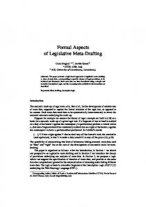182 Lagorio, Servetto and Zucca cp ce B fds fd mds md e :: = :: = :: = :: = :: = :: = :: = :: = class C = ce C | B | ce extends ce 0 {fds mds} fd T f; md T m(T x ) {return e; } x | e.f | e.m(e) | new C (e) | (C )e v :: = new C (v ) value T CT mhs mh ∆ Γ :: = :: = :: = :: = :: = :: = C hC , fds, mhsi mh T m(T ) C :CT x :T type (conventional) program class expression base class field declarations field declaration method declarations method declaration (runtime) expression class type method headers method header class type environment parameter type environment Figure 1. Syntax and types of the conventional language In this way the compilation of the same source produces customized versions of the library depending on the execution platform. In other words, this approach can be used to write active libraries [2], that is, libraries that interact dynamically with the compiler, providing better services, as meaningful error messages, library-specific optimizations and so on. 2 Formalization Figure 1 shows syntax, values and types of our conventional language, using the overbar notation to denote a (possibly empty) sequence. 9 The top section of the figure defines the syntax, where we assume infinite sets of class names C , field names f and method names m. As already mentioned, to keep the presentation minimal we consider a class composition language with only one operator, extends. This conventional language is very similar to Featherweight Java [6], FJ for short, but the operator extends composes two class expressions, rather than the name of an existing class with a class body (base class). Reduction rules are as in FJ and are omitted. The only difference is that look-up, formally expressed by the function mbody, needs to be generalized, as shown in Figure 2, to take into account that extends composes two class expressions. We omit the analogous trivial generalization of the function fields. Values v of the conventional language are as in FJ. 9 This notation for metavariables is the analogous of the Kleene-star in BNF style. 183 Lagorio, Servetto and Zucca (

Formal aspects of component software

Formal aspects of component software

Suggest Documents

IIST Formal Aspects of Component Software

Formal aspects of component software - Centrum Wiskunde ...

IIST Formal Aspects of Component Software

UNU/IIST Formal Aspects of Component Software ...

Formal aspects of component software - source url - CWI Amsterdam

Formal Methods for Component Software: The

Formal Verification of Component-Based Software ... - Semantic Scholar

A Formal Model for Component-Based Software - Faculty of ...

The Different Aspects of Component Based Software Engineering

Special Aspects of Component Based Software ... - Semantic Scholar

Formal Methods for Component Software: The Refinement ... - CiteSeerX

A Framework for Formal Component-Based Software Architecting

Formal Methods for Component Software: The ... - Semantic Scholar

Aspects of Software Adaptability

Formal Security Policy Verification of Distributed Component

Formal Aspects of Element Theory - Florian Breit

formal and functional aspects of phonological knowledge

Formal and Informal Aspects of Requirements

Formal Aspects of Legislative Meta-Drafting - ittig

EVALUATING TRUSTWORTHINESS OF SOFTWARE COMPONENT ...

Verification of Component-Based Software

Reengineering of Component-Based Software

Software Component Architecture - CIMNE

Tracking Component-Based Software