formal software measurement for object-oriented business models

FORMAL SOFTWARE MEASUREMENT FOR OBJECT-ORIENTED BUSINESS MODELS Geert Poels Prof. Dr. Guido Dedene Katholieke Universiteit Leuven Dept. of Applied Economic Sciences Naamsestraat, 69 B-3000 Leuven Belgium E-mail [email protected] Research Assistant of the Belgian National Fund for Scientific Research

Abstract - This paper presents a set of metrics and pseudo-metrics for the measurement of conceptual distances in M.E.R.O.DE. business models. The measures are developed and validated using measure and measurement theory. It is argued that this metrics set constitutes a strong formal basis for the further assessment and prediction of relevant internal and external attributes of object-oriented specifications. Keywords - object type, business model, conceptual distance, measure theory, measurement theory, metric, pseudo-metric, scale type, measure validation

I. INTRODUCTION In software engineering the notions of software metric and software measure are used interchangeably and mostly without reference to the mathematical discipline of measure theory and the philosophical discipline of measurement theory. In order to formalise the measurement of software, the distinction between a metric and a measure must be clarified and both terms must be used in a consistent manner. Formalisation of measurement implies that the principles of measurement theory, especially the representational approach to measurement theory, are adhered to. Recently quite a lot of efforts have been done in this direction. The work of Norman Fenton can be considered a milestone in this regard, as he is an enthusiastic promoter of sound measurement theoretical principles in software measurement research [7,8]. Basically, measurement is the assignment of numbers to entities [14]. Of course, this assignment is not arbitrary, it should conform to certain rules. Measurement theory states what conditions must be fulfilled to have good, valid measurement. For instance, for measurement on an ordinal scale, the numbers assigned to the entities should reflect the intuitive ordering of these entities based on the quantities of the attribute we wish to measure. Formally, to define a measure on an ordinal scale, we need to define [5,7,10,14]:

• An empirical relational system (A,R) consisting of a set A of entities and a set R of relations on A as can be observed in reality. The relations in R order the entities of A according to the inherent quantity of a certain attribute of these entities. • A numerical relational system (B,S) consisting of a set of numbers (e.g., the real numbers) and the usual ordering relations (e.g., ≤) on these numbers. • A measure which is a mapping µ from (A,R) into (B,S) such that ∀ a, b ∈ A: ∀ Ri ∈ R, ∃ Si ∈ S: a Ri b ⇔ µ(a) Si µ(b). This condition is called the representation condition of ordinal measurement. The representation problem is solved if the existence of a homomorphical mapping (i.e., a measure) from the empirical relational system into the numerical relational system is shown. The uniqueness problem involves the question: How unique is this homomorphical mapping? Solving the uniqueness problem means determining the scale type of the measure, which in turn defines the set of allowable mathematical operations on the measurement values. In the previous example an ordinal scale type was assumed. For other scale types other representation conditions must be satisfied. For instance, to measure on an interval scale the representation condition of difference measurement must be fulfilled. To measure on a ratio scale requires the problem of extensive measurement to be solved (see [14] for a good reference on measurement theory). These scientific principles must be applied in software measurement research. Formal measurement of software means solving the representation and uniqueness problems in the context of software engineering. A measure can only be introduced by explicitly defining what the empirical relational systems looks like, into which numerical relational system the entities are mapped, and how the attribute in question is quantified (i.e., the mapping function). All too often measures are proposed without clarification of these concepts. A critical review of these measures can, by making the underlying measurement model and assumptions explicit, reveal whether the measures are valid according to measurement theory (see for instance [13]).

Although the application of sound measurement theoretical foundations is gaining ground in software measurement, we did not find many references pointing to the application of mathematical measure theory in software measurement. In measure theory a measure is defined as a function on sets [2,11,15]. To define a measure first a measurable space needs to be identified. Formally, a measurable space (X,S) consists of a set X of entities and a σ-algebra S of subsets of X. The σalgebra S is a set of subsets of X that is closed for the intersection and the union operator. A measure µ is a non-negative set function on the σ-algebra S satisfying: • µ(∅) = 0 • µ(A) < µ(B) if A ⊂ B • µ(∪Ai) ≤ ∑µ(Ai) Also in measure theory the concept of a metric is defined. A metric is a function measuring the distance between two entities. In fact, a metric is distinguished from a pseudo-metric. A pseudo-metric is a non-negative function δ on two entities that satisfies the following conditions: • δ(x,x) = 0 (identity) • δ(x,y) = δ(y,x) (symmetry) • δ(x,y) ≤ δ(x,z) + δ(z,y) (triangle inequality) A metric is a pseudo-metric that satisfies a stronger axiom of identity: δ(x,y) = 0 ⇔ x = y Graham compares the definition of a metric and a measure to the actual use of the term software metric and software measure and concludes that “the use of the terms metric and measure in computer science is not usually as precise as this ...” [9, p. 400]. Fenton asserts that the concept of metrics in the sense of measure theory, which he calls ‘real’ metrics, can be reconciled with his software measurement framework based on measurement theory [7]. Although he gives examples of the use of ‘real’ metrics in the context of fault tolerance assessment, diversity of designs measurement and programspecification satisfaction, he does not elaborate the idea of using metrics any further. Dvorak proposes some metrics measuring aspects of conceptual entropy between Smalltalk object classes, but does not formally define these metrics [4]. The only reference we found in which principles of measure theory are really applied to software measurement is [6]. Ejiogu examines whether a tree-like model of software structure satisfies the requirements of measurable spaces. His fundamental theorem of software metrics ‘If T is a tree (structure) and S = {Ljk} is the class of nestings of parent-child nodes of T, then S is a σring’ is the ‘fundamental ground space for software metrics’ [6, p. 41]. Ejiogu applies these important findings only in the context of structured programming and the measurement of the structural complexity of software. Ejiogu proposes some measures, but he does not consider metrics, a more basic concept in measure theory that we shall consider.

In software engineering software metrics can be defined to measure conceptual distances (i.e., conceptual differences) between software entities. Based on these distances a framework can be introduced to formally define and measure a number of internal product attributes that are potentially useful for assessing and predicting relevant software product, process and resource attributes. By integrating concepts from measure and measurement theory, we believe a strong formal measurement basis can be created that guarantees the validity of the proposed measures. In this paper concepts of both theories are applied to software specifications developed using the object-oriented paradigm, and this as early as the business modelling phase. In section 2 the development methodology we use to model business object types and business models is briefly discussed. This methodology is M.E.R.O.DE., which is an acronym for Model-driven EntityRelationship Object-oriented DEvelopment. In section 3 a metric is developed that measures the conceptual distance between M.E.R.O.DE. business object types. In section 4 this metric is used to define a new metric measuring conceptual distances between M.E.R.O.DE. business models. In section 5 it is discussed how these software metrics enable the creation of a number of indirect measures of both internal and external attributes of relevant software entities. Also a few examples are given of how to derive these indirect measures and how they can be used in software measurement. Finally, in section 6 conclusions and future research directions are presented.

II. M.E.R.O.DE. To define a valid measure it must be exactly known how the empirical relational system looks like. In software engineering this is mostly not the case [19]. Software entities and their attributes are not formally defined and neither are the measures of these attributes. Even in Object Orientation, where the primary goal was to improve the quality of delivered software, most methodologies are characterised by a low level of formality [3]. However in M.E.R.O.DE. important software entity concepts are formalised by means of a process algebra [16]. It is this ability to formally define conceptual business models and their components that allows us to develop a strong measurement basis.

BOOK

MEMBER

LOAN

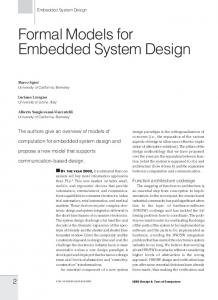
Figure 1: Object-Relationship Diagram Library example A M.E.R.O.DE. business model describes the functioning of the business in terms of object types, event types and the relationships between object types and event types [3]. The static aspect of such a business model is described by an Object-Relationship Diagram, which in fact integrates an Entity-Relationship Diagram and an Existence-Dependency Graph. Figure 1 shows an example of an O-R diagram (adapted from [16]). The diagram specifies that over time a book can be lend by many members, while a member can lend many books. Also the object type loan, which is a kind of contract between a book and a member, is existence dependent on both book and member, meaning that its life cycle is embedded in the life cycles of book and member. The dynamic aspects of a business model are described by the Object-Event Table and by Jackson Structure Diagrams. The Object-Event Table identifies the relevant event types for each of the business object types and specifies which events create, destroy or modify object occurrences [3]. In figure 2 an example Object-Event Table is shown. For each object type a Jackson Structure Diagram describes the sequence restrictions imposed on the event types that are relevant for the object type. Jackson Structure Diagrams are mathematically equivalent with Finite State Machines, a dynamic modelling technique used in many commercial OO development methodologies (e.g., OSA, OOSA, OOA) [16]. Figure 3 shows the JSD diagrams for the object types in the library example. Finally the other business constraints (e.g., referential integrity constraints) are formulated, and for each of the business object types attributes are defined. This results in the definition of abstract data types containing the state vector of the object type and one method for each event type in which the object type participates [3]. The abstract data types and the data constraints for the example are shown in figures 4 and 5.

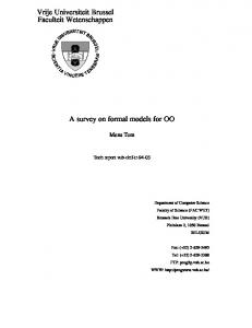
MEMBER BOOK LOAN Object-Event Table ENTER C LEAVE D ACQUIRE C CATALOGUE M SELL D LOSE M D D BORROW M M C RENEW M M M RETURN M M D Figure 2: Object-Event Table Library example In [16] a process algebra was developed to formalise conceptual business models. The universe of event types in the model is denoted by the set A. The subset of A that is relevant for a certain object type (i.e., containing the event types in which the object type participates) is called the alphabet of the object type. The alphabet of an object type is selected by the function SA. Example SAMEMBER = {enter, leave, lose, borrow, renew, return} SABOOK = {acquire, catalogue, sell, lose, borrow, renew, return} SALOAN = {borrow, renew, lose, return} By means of the operators ‘.’ (for sequence), ‘+’ (for selection), and ‘*’ (for iteration) regular expressions over A are built. The set R*(A) is the set of regular expressions over A. In [16] it is shown that R*(A),+,. is an idempotent semi-ring. The Jackson Structure Diagrams are graphical representations of these regular expressions. Hence, each object type’s life cycle is modelled by a regular expression. This regular expression is selected by the function SR. Example SRMEMBER = enter . (borrow + renew + return + lose)* . leave SRBOOK = acquire . catalogue . (borrow + renew + return)* . (sell + lose) SRLOAN = borrow . (renew)* . (return + lose) To summarise, each business object type P is formally modelled by a tuple (SAP, SRP) containing its alphabet and a regular expression over this alphabet. A conceptual business model is a set M of business object types that satisfy a number of restrictions (see [16] for a detailed account), the first of which is that the union of the alphabets of the object types in M must be the set A.

Figure 3: Sequence restrictions in the Library example

MEMBER State Vector Member-id, Member-state

BOOK State Vector Book-id, Book-state, Book-catalogue-number Methods Methods ENTER { ACQUIRE { Member-id := Book-id := ACQUIRE_book-id; ENTER_member-id; Book-state := “1”; Member-state := “1”; } } CATALOGUE { LEAVE { Book-catalogue-number := Member-state := “E”; CATALOGUE_book} catalogue-number; LOSE { Book-state := “2”; } } BORROW { SELL { } Book-state := “E”; RENEW { } } LOSE { RETURN { Book-state := “E”; } } BORROW { } RENEW { } RETURN { } Figure 4: Abstract Data Types Library example

LEAVE: All LOAN(Loan-member-id = LEAVE_member-id).Loan-state = “E” SELL: All LOAN(Loan-book-id = SELL_book-id).Loan-state = “E” Figure 5: Data Constraints Library example

LOAN State Vector Loan-id, Loan-member-id, Loan-book-id, Loan-state Methods BORROW { Loan-id := BORROW_Loan-id; Loan-member-id := BORROW_member-id; Loan-book-id := BORROW_book-id; Loan-state := “1”; } RENEW { Loan-state := “2”; } LOSE { Loan-state := “E”; } RETURN { Loan-state := “E”; }

III. A MEASURE OF CONCEPTUAL DISTANCE FOR BUSINESS OBJECT TYPES

since P and Q can differ on other aspects than just their alphabet.

Although in software measurement research many software metrics are proposed, few of them qualify as a metric. In this section the function δ(P,Q) is proposed for measuring the difference between M.E.R.O.DE. business object types P and Q. Since δ(P,Q) is a metric according to measure theory, it may be called a software metric without abusing existing mathematical concepts. At the end of this section it is shown that δ can be defined such that it is a valid measure of conceptual distance according to measurement theory. Since a non-empty set OM of M.E.R.O.DE. business object types and the distance function δ(P,Q): OM x OM → Re is said to form a metric space, it is common to call the difference between P and Q the (conceptual) distance from P to Q [11]. In subsequent research δ(P,Q) will be used to develop a topology on the set of object types. This topology can serve as a basis for further formal measurement of M.E.R.O.DE. specifications (e.g., the measurement of complexity viewpoints). In the previous section it was described that M.E.R.O.DE. business object types are composed of an alphabet of event types, a regular expression on these event types describing sequence constraints, a set of attribute types, and eventually, some data constraints [3,16]. To compare object types each of these aspects must be considered, i.e., object types can differ along each of these four dimensions. Since it does not seem possible at this moment to measure differences along the four dimensions simultaneously, first a number of pseudo-metrics are developed to measure conceptual distances on each of these dimensions separately. Next, the pseudo-metrics are combined to define a metric measuring the global difference between object types. In the next section this metric is used to indirectly measure the conceptual distance between business models.

B. Measuring differences in attribute set The difference in attribute set between two object types P and Q can be measured much the same way as the difference in alphabets. Let us introduce the selector SS for the attribute set of an object type. The conceptual distance measure for differences in attribute set is defined as δatr(P,Q) = cSSP ∆ SSQ. The symmetric difference of the sets SSP and SSQ is defined as SSP ∆ SSQ = (SSP - SSQ) ∪ (SSQ - SSP). The function c X maps the set X to its cardinality.

A. Measuring differences in alphabet The difference in alphabet between the object types P and Q is measured as the cardinality of the symmetric difference of the sets SAP and SAQ, where SA is the selector for the alphabet of an object type. Formally, δalph(P,Q) = cSAP ∆ SAQ , where the symmetric difference between two sets SAP and SAQ is defined as SAP ∆ SAQ = (SAP - SAQ) ∪ (SAQ - SAP) and c X  is a function mapping a set X to its cardinality. δalph(P,Q) is also called a measure of conceptual distance from the object type P to the object type Q. Conceptual distance and difference are equivalent terms in this context. Of course, the conceptual distance δalph(P,Q) is only one aspect of difference between P and Q. In measure theory distances are measured by metrics and pseudo-metrics. In appendix 1 it is shown that δalph(P,Q) is in fact such a pseudo-metric. It cannot be a metric

By analogy to δalph(P,Q) it can be shown that δatr(P,Q) is a pseudo-metric (see appendix 1) C. Measuring differences in sequence constraints In [16] sequence constraints are regular expressions on the alphabet of object types. Hence, the operands of sequence constraints are event types. Differences in alphabets between object types are captured by δalph. So, if we just compare the sequence constraints, the difference in alphabet is measured again. Of course, a sequence constraint is more than just the event types that are part of it. It is this additional aspect that must be measured. We may call this the structure of the sequence constraint. This structure consists of the operators (. for sequence, + for selection and * for iteration) and the order in which these operators are applied. To visualise the structure of sequence constraints the projection operator \seq : R*(A) → R*{x} : e → e \seq is defined such that a \seq = x (e.e’) \seq = e \seq . e’\seq (e+e’) = e \seq + e’ \seq (e*) \seq = (e \seq)* where a is an event type, e and e’ are regular expressions and x is a dummy event type on which every event type of the regular expression e can be projected such that the structure of e is not altered. The dummy event type x has no semantic meaning of its own. Example (see previous section) SRMEMBER\seq = x . (x + x + x + x)* . x SRBOOK\seq = x . x . (x + x + x)* . (x + x) SRLOAN\seq = x . x* . (x + x) The measure δseq(P,Q), which in fact should be written as δe\seq(P,Q) (but we shall employ the first notation for reasons of brevity), measures the difference in the \seqprojected sequence constraints between object types P and Q. Now, how can δseq(P,Q) be defined such that it adequately reflects differences in \seq-projected sequence constraints and satisfies the axioms of pseudo-metrics ?

First of all, every possible \seq-projected sequence constraint is made comparable by creating a ‘net’ of object types, in which every object type can be reached transformation t1: x → x.x

t2: x → x+x

t3: x → x*

t4: e.x → e

t5: x.e → e

t6: e+x → e

from

from any other object type by means of a limited and fixed set of allowable transformations. The transformations which are allowed are shown in figure 6. to

t7: x+e → e

t8: e* → e

Figure 6: Allowable transformations on \seq-projected sequence constraints The transformations t1, t2 and t3 expand the \seqprojected sequence constraints (i.e., the \seq-projected regular expression) of an object type. The transformations t4 until t8 compress the \seq-projected regular expression. By means of the transformations t1, t2 and t3 each object type with a valid life cycle can be derived from the object type with the trivial life cycle create.destroy. The life cycle of an object type is valid if instances of the object type can be created and destroyed. The meanings of t1, t2 and t3 are respectively the addition of a sequence, the addition of a selection and the addition of an iteration. The addition of these program structures can only happen in the manner described by the transformations. To transform an object type’s \seq-projected regular expression back into the trivial \seq-projected regular expression, we use transformations t4 until t8. The number of transformations needed to transform the object type with trivial life cycle into the \seq-projected regular expression of an object type P is equal to the number of transformations needed to transform the \seq-projected regular expression of P back into the \seq-projected regular expression of the trivial object type. This number of transformations is simply a count of the number of sequence, selection and iteration operators in the \seq-projected regular expression of P, minus 1 because there is already one sequence operator in the trivial life cycle. Since it is possible to ‘reach’ each object type starting from the trivial object type (i.e. object type with trivial life cycle) and, secondly, since it is always possible to find a way back from each object type to the trivial object type, it is possible to transform the \seq-projected regular expression of an object type into the \seq-projected regular expression of any other object type, at least as long as life cycles are valid. In the worst case we just find our way back to the trivial object type and go on to the desired object type. Since the 8 transformations add or delete sequence constraints every possible object type with a

valid life cycle can be compared. By counting the number of transformations needed we can measure how much the sequence constraints of two object types differ. The function δseq(P,Q) is defined as the minimum number of transformations needed to transform the \seq-projected regular expression of object type P into the \seq-projected regular expression of object type Q. When measuring the distance from an object type to the object type with trivial life cycle, this amounts to counting the number of sequence, selection and iteration operators (minus 1) in the \seq-projected regular expression of the object type. When both P and Q are different from the trivial object type, there are many ways to transform P into Q or Q into P. That is why the notion of minimum number is used. In appendix 2 it is shown that δseq(P,Q) is a pseudo-metric. Example SRBOOK\seq = x.x.(x+x+x)*.(x+x) t8(SRBOOK\seq) = x.x.(x+x+x).(x+x) t6(t8(SRBOOK\seq)) = x.x.(x+x).(x+x) t6(t6(t8(SRBOOK\seq))) = x.x.x.(x+x) t4(t6(t6(t8(SRBOOK\seq)))) = x.x.(x+x) t3(t4(t6(t6(t8(SRBOOK\seq))))) = x.x*.(x+x) = SRLOAN\seq δseq(BOOK,LOAN) = 5 D. Measuring differences in data constraints The data constraints imposed on an object type are strongly dependent on the event types in which the object type participates (a data constraint always refers to an event type) and on the attributes of the object type (sometimes additional attributes are needed to implement data constraints) [17]. Differences in data constraints are to a certain extent the logical result of differences in alphabets (event types) and attributes. If we do wish to measure differences in data constraints, we can define the measure δdata(P,Q) = cSDP ∆ SDQ, where SD is the selector for the set of data constraints that can be attributed to an object type, cXis the function mapping the set X to its cardinality, and the symmetric difference ∆ is defined in the usual way.

Note that since it is not expected that object types have data constraints in common, δdata(P,Q) is mostly equal to the sum of the number of data constraints in both object types. The axioms of pseudo-metrics are satisfied by δdata(P,Q), since it is defined as the cardinality of the symmetric difference between sets (see appendix 1). E. Characterisation as measures The attribute measured is conceptual difference, also called conceptual distance since it is measured by a pseudo-metric. Each pseudo-metric measures another viewpoint of this attribute. This means we have to identify four different empirical relational systems. However, the set of entities is always the same set. The attribute of difference is a special kind of attribute since it does not belong to one single entity. An entity cannot have a difference. A difference (or a distance) is always between two entities. So, it is more convenient to consider the attribute of difference as belonging to pairs of entities [7]. These entities are M.E.R.O.DE. business object types. Let us denote the set of M.E.R.O.DE. business object types we wish to measure as OM. An empirical relational system consists of a set of entities and a set of relations. The set of entities is OMxOM. We wish to measure the difference between any pair of object types in OM, hence the set of entities is the set of all pairs in OMxOM. Each of the component pseudo-metrics measures one aspect of difference. This implies there are four empirical relational systems, each consisting of the set OMxOM and (at least) one relation expressing an ordering on the pairs of object types according to the aspect of difference measured. Let us denote these relations by ≤i, where the subscript i can be replaced by alph (meaning alphabet), seq (meaning sequence restrictions), atr (meaning attribute set) and finally data (meaning data constraints). The relations ≤i are ordering relations. Suppose P, Q, R and S are object types belonging to OM. Suppose further that we wish to compare the difference in aspect i (i = alph, seq, atr or data) between the pairs (P,Q) and (R,S) belonging to OMxOM. Let us define the meaning of (P,Q) ≤i (R,S) as ‘the difference in i between P and Q is smaller or equal than the difference in i between R and S’. The numerical relational system the measures are mapped into consists of a set of numbers and a set of relations. It is convenient to use the set of real numbers Re as the set of numbers. Since the set of empirical relations is a singleton set, a single ordering relation ≤ (the same for each of the aspects) on the set of real numbers is used. To summarise, the empirical relational systems are defined as (OMxOM, ≤i), and the numerical relational system is (Re, ≤). It must now be shown that each of the pseudo-metrics δi is a homomorphic mapping from (OMxOM, ≤i) into (Re, ≤).

The pseudo-metrics δi (where i is alph, atr, seq and data) are homomorphic mappings (i.e., valid measures according to measurement theory) from the empirical relational system into the numerical relational system if they satisfy the representation condition. For ordinal measurement this means that ∀ (P,Q), (R,S) ∈ OMxOM: (P,Q) ≤i (R,S) ⇔ δi(P,Q) ≤ δi(R,S) A variant of the representation theorem of Cantor states the axioms that are necessary and sufficient to prove the existence of a homomorphic mapping from (OMxOM,≤i) into (Re, ≤) [14, p. 107]: “ Suppose A is a finite set and R is a binary relation on A. Then there is a real-valued function f on A satisfying aRb ⇔ f(a) ≤ f(b) if and only if (A,R) is a weak order”. The relation ≤i is a binary relation on the finite set OMxOM. The empirical relational system (OMxOM, ≤i) is a weak order if: • ≤i is transitive • ≤i is strongly complete Representation theorems can be interpreted in two manners [14]. If we take the descriptive approach, we must examine whether the axioms of transitivity and strongly completeness are satisfied in the real world. Since it is not easy to empirically check whether the axioms are satisfied, we take the normative or prescriptive approach which just assumes that the axioms are true [14]. The normative approach defines rationality in (OMxOM, ≤i). Measurement is restricted to those empirical relational systems that are rational. Hence, the relations ≤i must be transitive and strongly complete. Note that these are very rational assumptions for any notion of difference or distance. To know that a homomorphical mapping exists from (OMxOM, ≤i) into (Re, ≤) is one thing. We also must show that δi is such a mapping. For our empirical relational systems this step is quite trivial because the conceptual differences between object types are made visible by our measurements. In other words we define (P,Q) ≤i (R,S) as δi(P,Q) ≤ δi(R,S). Hence, the representation conditions are by definition satisfied. We may conclude therefore that the component pseudometrics are valid measures of conceptual difference or distance according to measurement theory. Note that by defining the pseudo-metrics as homomorphisms we have in fact defined viewpoints for the attributes measured. These viewpoints depend on the way the pseudo-metrics are calculated. If the pseudometrics change, the viewpoints also change, and other representation conditions involving other empirical relational systems will be satisfied. F. Scale type of the pseudo-metrics The representation condition and theorem used so far guarantee an ordinal scale type. Ordinal scales are not very useful. We would like to characterise our

measurement on higher, more useful scales like e.g., the ratio scale. Ratio scales require other axioms to be fulfilled. In general, ratio scales are used in extensive measurement, which requires in turn the existence of a binary operation on the elements of the empirical relational system. This binary operation combines two elements into a third element, which is also part of the empirical relational system. We think however that it is not appropriate to create a combination-operator for business object types. It is not intuitively clear whether the combination of two business object types will result in another meaningful business object type. Such a combination-operator can certainly be developed, but it is questionable whether this is part of the empirical relational systems we are used to work with. The combination of two object types requires more than just putting the two object types together if we want the result to be a meaningful object type. So we will not try to transform our measurement system into an (explicit) extensive one, although theoretically this could be done. Even without extensive measurement and explicit binary operations on object types it can be shown that we have in fact a ratio scale instead of an ordinal scale. This is because we only used Cantor’s theorem in showing that we have an ordinal scale. The component measures of distance also satisfy the axioms of pseudometrics. These axioms force our measurements to be on a ratio scale. Every scale type has a class of admissible transformations which can be applied without changing the properties of the scale. An admissible transformation of a scale leads to another scale of the same type. Figure 7 lists the types of scale and the corresponding classes of admissible transformations. class of admissible transformations φ(x)=x (identity) φ(x)=a.x, ∀a > 0 similarity transformation φ(x)=a.x+b, ∀a > 0 positive linear transformation x ≤ y ⇔ φ(x) ≤ φ(y) monotone increasing transformation any one-to-one φ Figure 7: types of scale [14, p. 64]

scale type absolute ratio interval ordinal nominal

Note the hierarchy in the scale types. On top are the most useful scale types, at the bottom are the least useful scale types. The class of admissible transformations gets smaller if we go to the more useful scale types. The scale type of the pseudo-metrics is assessed by transforming them and examining whether the transformed measures still satisfy the axioms for pseudometrics. We shall begin with the smallest class of transformations (for an absolute scale) and extend this class until the point where the axioms are no longer satisfied. Let δi(x,y) be an arbitrary component pseudometric measuring the conceptual distance from object

type x to y along a certain dimension i (alphabet, sequence constraints, ... ), and let x, y and z be object types belonging to OM. Absolute scale The class of admissible transformations is φ(δi(x,y)) = δi(x,y). This means that only the identity transformation is allowed. The three axioms for pseudo-metrics are therefore trivially satisfied. Ratio scale The class of admissible transformations is φ(δi(x,y)) = a.δi(x,y), ∀ a > 0. • a.δi(x,x) = a.0 = 0 • a.δi(x,y) = a.δi(y,x) ⇒ δi(x,y) = δi(y,x) • a.δi(x,y) ≤ a.δi(x,z) + a.δi(z,y) ⇒ a.δi(x,y) ≤ a.(δi(x,z) + δi(z,y)) ⇒ δi(x,y) ≤ δi(x,z) + δi(z,y) Interval scale The class of admissible transformations is φ(δi(x,y)) = a.δi(x,y) + b, ∀ a > 0 • a.δi(x,x) + b = a.0 + b ≠ 0 • a.δi(x,y) + b = a.δi(y,x) + b ⇒ a.δi(x,y) = a.δi(y,x) ⇒ δi(x,y) = δi(y,x) • a.δi(x,y) + b ≤ a.δi(x,z) + b + a.δi(z,y) + b ⇒ a.δi(x,y) + b ≤ a.(δi(x,z) + δi(z,y)) + 2.b ⇒ δi(x,y) ≤ δi(x,z) + δi(z,y) + b Clearly, axioms 1 and 3 are not satisfied if b has an arbitrary value. We conclude that the scale type of the measures is ratio. Note that we reached this conclusion not by using the representation theorems of measurement theory, but by the important property that our measures are pseudometrics. The axioms for pseudo-metrics impose a ratio scale on the component measures of distance. The only transformations allowed are scalar multiplications. G. Measurement protocols Apart from a measure’s definition, procedures are needed that lead to consistent measurement of the attributes of an entity. These procedures are part of what Kitchenham et al. call the measurement protocol [12]. This protocol contains the model of the entity on which measurement is based, and the procedures, guidelines and rules to carry out the actual measurement. As far as models are concerned, entity abstractions for the pseudo-metrics measuring conceptual distances between object types, have already been identified. These entity abstractions are the alphabet, the attribute set, the \seq-projected sequence constraints, and the set of data constraints of an object type. The object type itself was modelled by a number of abstractions prescribed by the M.E.R.O.DE. methodology. However, the specific measurement procedures for each pseudometric were not described. They are nonetheless important because actual measurement should be

independent of environment and the person carrying out the measurement [12]. In this paper we are more concerned about the conceptual definition of the measures than we are interested in their measurement protocols. Anyway, most pseudo-metrics can be straightforwardly calculated. H. Example For the library example of section 2, the measurement values of conceptual distance aspects are: 1. The conceptual distances in alphabet are: δalph(MEMBER, BOOK) = 5 δalph(MEMBER, LOAN) = 2 δalph(BOOK, LOAN) = 3 2. The conceptual distances in attribute set are: δatr(MEMBER, BOOK) = 5 δatr(MEMBER, LOAN) = 4 δatr(BOOK, LOAN) = 5 (Note that we considered Member-id = Loan-member-id and Book-id = Loan-book-id) 3. The conceptual distances in \seq-projected sequence constraints are: δseq(MEMBER, BOOK) = 9 (transformations: t1, t2, t8, t6, t6, t6, t2, t2, t3) δseq(MEMBER, LOAN) = 6 (transformations: t8, t6, t6, t6, t3, t2) δseq(BOOK, LOAN) = 5 (transformations: t8, t6, t6, t4, t3) 4. The conceptual distances in data constraints are: δdata(MEMBER, BOOK) = 0 δdata(MEMBER, LOAN) = 2 δdata(BOOK, LOAN) = 2

I. A metric for measuring the global conceptual distance between object types In this subsection a global measure of conceptual distance from the business object type P to the business object type Q is derived. First the global measure δ is represented as a scalar. Next, an alternative definition of δ as a vector is presented. Finally, the pros and cons of each type of representation are evaluated. 1. Scalar representation Suppose a global measure of difference between object types is defined as a linear combination of the four earlier developed component measures. Formally, δ(P,Q) = aalph.δalph(P,Q) + aseq.δseq(P,Q) + aatr.δatr(P,Q) + adata.δdata(P,Q) where aalph, aseq, aatr and adata are constants and P and Q are object types belonging to the set of M.E.R.O.DE. object types OM. It can be shown that δ(P,Q) is a pseudo-metric (see appendix 3). δ(P,Q) is also a metric because it measures

conceptual distances from P to Q for all four possible aspects of difference. A metric has to satisfy the stronger version of the identity axiom. Formally, δ(P,Q) = 0 ⇔ P=Q. The proof in the ⇐ direction is trivial since this is in fact the weaker axiom of identity. For the proof in the ⇒ direction it suffices to notice that when two object types P and Q do not differ on any of the four aspects, i.e., δi(P,Q) = 0 for subscript i = alph, seq, atr and data, then δ(P,Q) = 0 and P is just a renaming of Q. So, if P and Q have the same alphabet, sequence constraints, attributes and data constraints, we may assert that they are identical object types. This proves that δ(P,Q) is a metric according to measure theory. We also wish to characterise the metric δ(P,Q) as a valid measure according to measurement theory. The component measures of distance δi(P,Q) are direct measures of the attribute difference along dimension i. A direct measure of an attribute does not depend on measures of other attributes [7]. Hence, no other attributes must be measured to know the value of δi(P,Q). The metric δ(P,Q) is not a direct measure. Its value depends on the values of the δi(P,Q)’s. The measurement of the global difference between object types involves the measurement of various aspects of this difference. Therefore δ(P,Q) is an indirect measure of difference between object types. According to [5] an indirect measure involving two or more direct measures is a derived measure. Hence, we shall also speak of δ(P,Q) as a derived measure. A derived measure has a derived scale. The type of a derived scale can be determined the same way as was done for direct measures. Note first that each of the component measures is multiplied by a constant representing its weight. Since the component measures are pseudo-metrics, measured on a ratio scale, a multiplication by a constant is an admissible transformation of scale. This means for instance that aalph.δalph(P,Q) is just a rescaling of δalph(P,Q). The scale type in both cases is ratio. A transformation of a derived scale is admissible (in the wide sense) if and only if there exist admissible transformations of the composing direct measures which still satisfy the equation relating the derived scale with the composing direct measures [14]. For δ the equation δ(P,Q) = aalph.δalph(P,Q) + aseq.δseq(P,Q) + aatr.δatr(P,Q) + adata.δdata(P,Q) must be satisfied. We now have to define the class of admissible transformations. Suppose δ is multiplied by the scalar A > 0. Now it is easily seen that we just have to multiply each of the composing direct measures by the same A, and the equation is satisfied.

A.δ(P,Q) = A.aalph.δalph(P,Q) + A.aseq.δseq(P,Q) + A.aatr.δatr(P,Q) + A.adata.δdata(P,Q) ⇔ A.δ(P,Q) = A.(aalph.δalph(P,Q) + aseq.δseq(P,Q) + aatr.δatr(P,Q) + adata.δdata(P,Q)) ⇔ δ(P,Q) = aalph.δalph(P,Q) + aseq.δseq(P,Q) +aatr.δatr(P,Q) + adata.δdata(P,Q) Next, we examine if it is possible to extend the class of admissible transformations to the form Φ(x)=ax+b. If such a transformation on the derived measure is allowed, i.e., there exist admissible transformations on the composing direct measures that satisfy the equation, then δ is not characterised by a ratio scale. However, the only admissible transformations of scale allowed on the composing direct measures are scalar multiplications. Previously was shown that they are measured on a ratio scale because they satisfy the properties of pseudometrics. So it is not possible to satisfy the equation when δ is transformed as if it were characterised by an interval scale. We conclude that the class of admissible transformations on the derived scale is Φ(x)=a.x (a>0). The type of the derived scale is ratio. Note that we would have reached the same conclusion by examining the class of admissible transformations on metrics. So far, it was shown that δ represented as a scalar is a metric according to measure theory, and is measured on a ratio scale. However, we did not show that δ is a valid measure according to measurement theory. According to [14] not every measurement theorist considers derived measures as valid measures. Authors like Roberts, Suppes and Zinnes consider any measure which is defined in terms of direct measures as a valid derived measure [14]. This means that there has to be a derived measurement function (until now called the equation) that relates the derived measure to the direct measures. The mere fact that such a derived measurement function exists, validates the derived measure, as long as, measurement values are calculated using this function. However, we must agree with Causey that the measurement function of derived measurement alone is not enough because ‘the derived scale is not required to reflect in any direct manner the characteristics of empirical relational systems’ (citation from [14, p. 77]). Also recently, in software measurement research, more stringent conditions are proposed. In [12] an indirect measure is considered valid if and only if the measurement function itself, relating indirect and direct measures, is validated. This may be done empirically, but preference is given to theoretical validations. The equation δ is based on, has no theory to support it, nor has the function (including the values chosen for the weight constants) been empirically shown to exist.

2. Vector representation The global measure of conceptual distance can alternatively be defined as a vector of the component measures of distance. Hence, ∀ P, Q ∈ OM: δ(P,Q) = (δalph(P,Q), δatr(P,Q), δseq(P,Q), δdata(P,Q)) According to [12] a vector cannot be transformed into a single scalar value by an arbitrary mathematical function. The relationship between the vector components must be based on a model if they are used to produce a scalar indirect measure, like we previously defined δ. Validating an indirect measure means validating the underlying model of the definition of the measure. While the theoretical validation of a measure is a complex issue in software measurement, empirical validations are not applicable since δ is not used to predict the conceptual distance, but to assess it. Moreover, empirically validating a measure means that some other direct measure of the attribute should be available. Methods exist to corroborate a measure empirically [12], but due to the lack of consensus concerning software attributes and the limited intuitive understanding of empirical relations between software products [19], this track is not elaborated any further. Validating a vector should be easier than validating a scalar indirect measure. However, the framework for software measurement validation of Kitchenham, Pfleeger and Fenton does not state how to validate an indirect measure that is a vector of direct measures [12]. We believe such an indirect measure is invalid if at least one of the vector components is not a valid measure of the attribute it is purported to measure. The model underlying the vector definition of δ is that the conceptual distance between object types has four dimensions. If differences along each of these dimensions are measured, then the global distance is measured. This model is valid if no other aspect of difference exists that can influence the global difference between object types. Hence, the theoretical model underlying the vector definition of δ assumes that linguistic differences in object type names are not relevant for the conceptual distance between object types. Whenever for object types P and Q, the component pseudo-metrics are all zero, P and Q can be considered the same object type, even when their names are different. Note that it was this argument that lead us to conclude that δ defined as a scalar is a metric and not just a pseudo-metric. The theoretical model also assumes, for example, that for object types P and Q having each a method in their abstract data types that is triggered by the same event type E, differences in the statements of the methods are not relevant for the conceptual distance between P and Q. Besides, these differences are partly reflected by δatr(P,Q) since the sequential statements in the methods modify the value of the attributes in the abstract data types state vectors. If the underlying theoretical model is valid and if all component measures are valid direct measures of aspects of difference, the indirect measure δ defined as a

vector is a valid measure of the conceptual distance between object types. Hence, as a vector δ is a valid indirect measure according to measurement theory. Let us now examine the properties of δ defined as a vector. First, what is the type of scale of δ? In [18] a number of indirect measures of control flow complexity which were based on pairs of direct complexity measures are validated. Zuse asserts that if ≤c is an empirical relation meaning ‘is less or equally complex than’, and P and P’ are programs, then P ≤c P’ ⇔ (µ1(P), µ2(P)) ≤ (µ1(P’), µ2(P’)) ⇔ µ1(P) ≤ µ1(P’) ∧ µ2(P) ≤ µ2(P’) If we extend this reasoning to vectors, then a vector A is smaller than or equal to a vector B whenever every vector component value ai in A is smaller than or equal to every corresponding vector component value bi in B. However for arbitrary vectors A and B, there is a non negligible chance that neither A ≤ B, nor B ≤ A. For the object types P, Q, R, S ∈ OM, the conceptual distance from P to Q is less than or the same as the conceptual distance from R to S (hereafter written as (P,Q) ≤cd (R,S) ) if and only if δ(P,Q) ≤ δ(R,S). If δ is defined as a vector, then δ(P,Q) ≤ δ(R,S) ⇔ δi(P,Q) ≤ δi(R,S) for i = alph, atr, seq and data. Again it is clear that uncomparabilities can arise. The binary relation ≤cd is reflexive and transitive. Hence, we have a quasi order [14]. It is however not strongly complete since it is not always true that δ(P,Q) ≤ δ(R,S) or δ(R,S) ≤ δ(P,Q). Thus, there is no weak ordering. Even the property of antisymmetry necessary for a partial ordering, is not satisfied. This implies that we cannot use representation theorems to assess the scale type of the measure. According to Zuse, indirect measures based on a vector have a scale type called half-ordering scale [18]. A half-ordering scale is somewhere between the nominal and the ordinal scale types in the scale hierarchy. This simply means that although the global conceptual distance of some pairs of object types can be compared, not all of them are comparable. So, using a half-ordering scale, pairs of object types can be ranked, but many rankings are possible, and none of them will comprise all object type pairs. It was shown that the vector components are pseudometrics. Can it now be asserted that δ is a pseudo-metric, or even a metric? ∀ P, Q ∈ OM: • If δ(P,Q) = (0,0,0,0) ⇒ P = Q since the theoretical model underlying δ is valid. If P = Q ⇒ δ(P,Q) = (0,0,0,0) since the vector components are pseudo-metrics. Hence, δ(P,Q) = (0,0,0,0) ⇔ P = Q This property is similar to the identity axiom of metrics.

• δ(P,Q) = (δalph(P,Q), δatr(P,Q), δseq(P,Q), δdata(P,Q)) = (δalph(Q,P), δatr(Q,P), δseq(Q,P), δdata(Q,P)) = δ(Q,P) since the vector components are pseudo-metrics. This property is the symmetry axiom of metrics. • Since the vector components are pseudo-metrics, ∀ R ∈ OM: δi(P,Q) ≤ δi(P,R) + δi(R,Q), for i = alph, atr, seq, data If the sum of two vectors is defined as the vector of the sum of the vector components, then it follows that δ(P,Q) ≤ δ(P,R) + δ(R,Q). This property is the triangle inequality. It is concluded that δ as a vector satisfies a number of properties similar to the metric axioms. However, the triangle inequality is only fulfilled it the sum of two vectors is defined as the vector of the sum of vector components. 3. Evaluation The scalar definition of δ satisfies the metric properties and is measured on a ratio scale. This means that each pair of object types can be mapped to a unique measurement value, on which the many kinds of operations associated with ratio scales are applicable. It is very tempting to represent the conceptual distance between object types this way. However, as shown earlier, the validity of such a definition cannot be proven. On the other hand, the vector definition of δ is shown to be valid according to measurement theory. But, in this case, measurement of conceptual distance does not result in a single measurement value, and uncomparabilities are created since δ is characterised by a half-ordering scale. So, from a pragmatical point of view, the scalar definition would be preferred. From a more scientific viewpoint, the vector definition is preferred. In subsequent research, the vector definition will be used, unless there is a theory supporting the use of scalar representations, or for purposes of measuring other attributes a single conceptual distance value is needed. 4. Example If δ is represented as the vector (δalph, δatr, δseq, δdata) then the conceptual distances are: δ(MEMBER, BOOK) = (5,5,9,0) δ(MEMBER, LOAN) = (2,4,6,2) δ(BOOK, LOAN) = (3,5,5,2) According to these measurement values, no definitive comparisons of conceptual distance can be made. It is however possible to compare the conceptual distances for each of the vector components separately. If δ is represented as a scalar by linearly combining the vector components, we get: δ(MEMBER, BOOK) = calph .5 + catr .5 + cseq .9 + cdata .0 δ(MEMBER, LOAN) = calph .2 + catr .4 + cseq .6 + cdata .2 δ(BOOK, LOAN) = calph .3 + catr .5 + cseq .5 + cdata .2

For all constants equal to 1 (i.e., all aspects of difference are equally important), we get: δ(MEMBER, BOOK) = 19 δ(MEMBER, LOAN) = 14 δ(BOOK, LOAN) = 15 Note however that the scalar representation of δ cannot be proven to be a valid measure, since the underlying measurement model (the linear combination, and the choice of the constant values) has not been shown to be valid. At most this model has an intuitive justification, meaning that the measured values correspond to a specific viewpoint of conceptual distance.

IV. MEASURING CONCEPTUAL BETWEEN BUSINESS MODELS

DISTANCES

A dynamic conceptual schema Μ is a set of object types that satisfies a number of constraints. For a detailed account of these constraints see [16]. The difference between two object types P and Q is measured by δ(P,Q). It was shown that this measure of conceptual distance satisfies the axioms of pseudo-metrics and metrics. We now wish to develop a measure of distance for dynamic conceptual schemes. This new measure should also be a pseudo-metric, and, preferably, be a metric. Equally important, the measure should be a valid measure according to measurement theory. A. Development of the measure The function δM(ΜP,ΜQ) must adequately reflect conceptual distances between schemes. The notion of conceptual distance can be defined in many ways. Each definition can be considered as a viewpoint of difference. The notion of viewpoints is extensively used in [18,19] to prove representation conditions for measurement. In the next subsection the viewpoint used is formally defined. In this subsection the measure is developed. Let us define δM(ΜP,ΜQ) as: δM(ΜP,ΜQ) = 0 I

J

∑ ∑ δ (P , Q ) i

=

⇔ ΜP ∆ ΜQ = ∅

i =1 j =1

j

⇔ ΜP ∆ ΜQ ≠ ∅

I. J where: ΜP and ΜQ are non-empty dynamic conceptual schemes; ΜP ∆ ΜQ = ∅ ⇔ (∀ P ∈ ΜP, ∃ Q ∈ ΜQ : δ (P,Q) = 0) ∧ (∀ Q ∈ ΜQ, ∃ P ∈ ΜP : δ (Q,P) = 0); cardinality (ΜP) = I; cardinality (ΜQ) = J; P i ∈ ΜP i = 1, ..., I; j = 1, ..., J; P j ∈ ΜQ

The above definition can be used for both scalar and vector representations of the measure δ(Pi,Qj). If δ is a scalar (i.e., δ(Pi,Qj) = aalph.δalph(Pi,Qj) + aseq.δseq(Pi,Qj) + aatr.δatr(Pi,Qj) + adata.δdata(Pi,Qj) ) then the expression I

J

∑ ∑ δ (P , Q ) i

j

i =1 j =1

is straightforwardly solved.

I. J

If δ is a vector (i.e., δ(Pi,Qj) = (δalph(Pi,Qj), δseq(Pi,Qj), δatr(Pi,Qj), δdata(Pi,Qj)) ) then the expression I

J

∑ ∑ δ (P , Q ) i

i =1 j =1

j

is equal to

I. J I J  I J   ∑ ∑ δalph( Pi , Qj ) ∑ ∑ δatr( Pi , Qj )  i = 1 j =1  i =1 j =1  ,   I. J I.J  I' J'  I J  δseq( Pi , Qj ) ∑ ∑ δdata( Pi , Qj ) ∑ ∑  i =1 j = 1  i =1 j = 1 ,  ,   I. J I. J

and for the case ΜP ∆ ΜQ = ∅, δM(ΜP,ΜQ) = (0,0,0,0). It can be shown that δM satisfies the axioms of metrics, or similar ones for vector representations (see appendix 4). The measure of distance δM is equal to the average distance between the object types of two different, nonempty dynamic conceptual schemes. A large average distance between object types leads to a large difference between the dynamic conceptual schemes. If the schemes are not different, then the measure is zero by definition. The identity axioms are by definition true. The schemes may however not be empty. For empty schemes the measure cannot be calculated. We believe this restriction will not hamper the usability of the measure. B. Validity of the measure The metric δM is a derived measure based on the I.J direct measures δ(Pi,Qj). According to [7,14] a derived measure is a valid measure. However, in section 3 we argued that a derived measure is valid only as long as the indirect measurement model it is based on is valid, and the direct measures it is composed of are valid. The validity of the pseudo-metrics has been shown in section 3. An indirect measurement model can be theoretically or empirically proven. The model is valid if the theory underlying the model is validated [12]. Informally, this theory can be stated as the conceptual distance between two conceptual schemes is the average distance between the object types in the schemes. This means that the validity of the measurement model is trivially shown if the attribute of conceptual distance is defined according to this theory.

Formally, the components of the measurement system are: • The empirical relational system Ε = (ΥxΥ, R), where Υ is a non-empty, countable set of non-empty dynamic conceptual schemes, ΥxΥ is the set of all conceptual schema pairs and R = {‘are closer to each other than’} is a singleton set of relations defined on ΥxΥ; • The numerical relational system Ν = (Re, 0. This multiplication is an admissible transformation of scale. If we multiply the derived measure by a constant A>0, we can multiply each of the terms by this constant A and still satisfy the condition. Since the δ’s are metrics, a scalar multiplication is the only admissible transformation. Hence, the derived measure has a ratio scale. Vector representation If the δ’s are defined as vectors, the scale of δM can at most be a half-ordering scale.

V. USING THE SOFTWARE METRICS Empirical relational systems related to software are not easily understood. Most of the time it is not known how these systems really look like [19]. Attributes like size, complexity and functionality are very general concepts that lack formal definitions, mainly because there exists little theory in software engineering [1]. Nonetheless, a lot of research was conducted to measure these concepts. However, if it is not known how the attributes are defined, you cannot develop valid measures for them. Using the formal measurement basis developed in this paper, internal attributes of M.E.R.O.DE. business object types and M.E.R.O.DE. business models can be formally defined. First we need to define a null object type showing only a minimal amount of the attribute that must be defined. The conceptual distance from an object type to this null object type determines the amount of the attribute that is present in the object type. Of course, it must also be determined which aspects of conceptual distance are considered. Next, the attribute is measured using the (pseudo-)metric(s) that measure the relevant conceptual distance aspects. This implies that once an attribute is formally defined, deriving a measure for the attribute is a trivial problem. If we wish, for instance, to measure the size of a M.E.R.O.DE. business object type, then this size attribute can be defined as the conceptual distance in alphabet and attribute set from an object type to the null object type. By formally defining the internal attributes of software products, we explicitly describe our viewpoints of these attributes. For size, it is the difference with an object type having no (or minimal) size that determines how much of the attribute is present. The definition

implies also that only differences in attribute set or alphabet are important to describe size differences. Once the attribute defined a measure is easily derived. For instance, the size of M.E.R.O.DE. business object types can be measured by the function size, which is defined as size(P) = (δalph(P,Null), δatr(P,Null)), where P is a M.E.R.O.DE. business object type and Null is the null object type. It can be shown that size is a valid measure of the attribute size such as defined above. Also, size has a meaningful scale type (i.e., the half-ordering scale). If the function size is defined as a linear combination of δalph(P,Null) and δatr(P,Null), it can be shown that the scale type of size is ratio. However as a scalar the measure validation is more difficult (see the discussion in section 3). Apart from the measurement of internal attributes of M.E.R.O.DE. business object types and models, the software metrics and pseudo-metrics can be used to predict relevant attributes of software products and processes. For prediction purposes we might think of a two-step approach. First the metrics are used to measure a number of internal attributes of object types and models, in the way described in the previous paragraph. Next, the measurement values of these attributes are the input variables of a model predicting the value of some dependent variable. Of course, the validity of such a prediction model does not only depend on the validity of the measures of the independent variables. More important for prediction purposes is the accuracy of the model, which must be established by empirical means, just as the model itself is empirically constructed (unless some theory guides the model construction). We also have identified a number of applications in which measures of conceptual distance can be directly used, mainly for assessment. Promising is the application of the metric δM to decide whether a conceptual schema is different from the schemes already present in a reuse repository. By calculating the values of δM the reuse potential of the schema is assessed. If necessary, the schema is included in the repository. Another possible application is case-based reasoning. Conceptual distances must be measured to retrieve closest-matching cases or nearest-neighbours in the case base. Software metrics, when properly defined, can measure these distances.

VI. CONCLUSIONS AND FURTHER RESEARCH In this paper a set of software metrics and measures was proposed for measuring the business object types contained in a M.E.R.O.DE. business model. M.E.R.O.DE., which is an acronym for Model-driven EntityRelationship Object-oriented Development, is an objectoriented development methodology with a high degree of formality. The formal definition of the conceptual business model and its components allowed us to develop

a formal measurement basis. Although the measures proposed in this paper are specifically developed for M.E.R.O.DE., we believe our measurement approach is generic and can be applied to any development methodology that models relationships, abstract data types, constraints, Finite State Machines, etc. Of course, the more formal the methodology, the easier the measures are derived. First a software metric was presented for measuring the conceptual difference between business object types. As object types can differ along a number of dimensions (e.g., attribute types, participation in event types, etc.), the difference along each of these dimensions was measured. It was shown that i) these component measures are pseudo-metrics according to measure theory, i.e., they are non-negative functions on two variables satisfying the axioms of weak identity, symmetry and triangle inequality, ii) they are valid direct measures according to measurement theory, and iii) the type of their scales is ratio. By combining the component measures of difference a global measure of conceptual distance between business object types was created. This global measure is both a metric according to measure theory (i.e., a pseudo-metric satisfying a stronger axiom of identity) and a valid indirect measure according to measurement theory, at least when defined as a vector. It was demonstrated that the scale type of the global measure is ratio when defined as a scalar, and half-order when defined as a vector. Next, an indirect measure of the difference between conceptual business models based on the notion of average distance between the object types contained in the models was discussed. Again it was shown that this measure is a metric with a ratio scale type (for scalars) or a half-ordering scale type (for vectors). Further research includes the development of a measurement framework for object-oriented specifications developed using M.E.R.O.DE. The metrics set constructed so far is the formal basis for such a framework. We believe the set must be extended in three directions. • In-depth by formulating measurement protocols for each of the pseudo-metrics. • Horizontally by developing measures of conceptual distance for other kinds of object types and models (e.g., for information and function object types, and for the information and technology model in M.E.R.O.DE.). • Vertically by formally defining and measuring other relevant attributes of M.E.R.O.DE. products, processes and resources in terms of conceptual distances.

VII. REFERENCES [1] Briand L., S. Morasca and V. Basili, ‘PropertyBased Software Engineering Measurement’, IEEE Transactions on Software Engineering, Vol. 22, No. 1, 1996, pp. 68-68. [2] DeBarra G., Introduction to Measure Theory, Van Nostrand Reinhold Company, London, 1974, 287 pp. [3] Dedene G. and M. Snoeck, ‘M.E.R.O.DE.: A Model-driven Entity-Relationship Object-oriented Development method’, ACM SIGSOFT Software Engineering Notes, Vol. 19, No. 3, 1994, pp. 51-61. [4] Dvorak J., ‘Conceptual Entropy and Its Effect on Class Hierarchies’, IEEE Computer, Vol. 27, No. 6, 1994, pp. 59-63. [5] Ellis B., Basic Concepts of Measurement, Cambridge University Press, 1968, 220 pp. [6] Ejiogu L.O., ‘Beyond Structured Programming: An Introduction to the Principles of Applied Software Metrics’, Structured Programming, No. 11, 1990, pp. 27-43. [7] Fenton N.E., Software Metrics, A Rigorous Approach, Chapman & Hall, London, 1991, 337 pp. [8] Fenton N.E., ‘Software Measurement: A Necessary Scientific Basis’, IEEE Transactions on Software Engineering, Vol. 20, No. 3, 1994, pp. 199-206. [9] Graham I, Migrating to Object Technology, Addison-Wesley, Wokingham, 1995, 552 pp. [10] Gustafson D.A., J.T. Tan and P. Weaver, ‘Software Measure Specification’, ACM Software Engineering Notes, Vol. 18, No. 5, 1993, pp. 163-168.

[11] Kingman J.F.C. and S.J. Taylor, Introduction to Measure and Probability, Cambridge University Press, 1966, 401 pp. [12] Kitchenham B., S.L. Pfleeger and N.E. Fenton, ‘Towards a Framework for Software Measurement Validation’, IEEE Transactions on Software Engineering, Vol. 21, No. 12, 1995, pp. 929-944. [13] Poels G. and G. Dedene, ‘Formal Measurement in Object-Oriented Software’, Workshop presented at OT96, Oxford, UK, March 25-27 1996. [14] Roberts F. S., Measurement Theory with Applications to Decisionmaking, Utility, and the Social Sciences, Addison-Wesley Publishing Company, Reading, 1979, 420 pp. [15] Royden H.L., Real Analysis, Macmillan Publishing Company, New York, 1968, 349 pp. [16] Snoeck, M., On a Process Algebra Approach for the Construction and Analysis of M.E.R.O.DE.-Based Conceptual Models, Phd dissertation, departement Computerwetenschappen, K.U.Leuven, 1995, 209 pp. [17] Verhelst M., ‘Model Based Entity-Relationship Object Oriented Development (M.E.R.O.DE.)’, Beleidsinformatica Tijdschrift, Vol. 20, No. 4, 1994, 51 pp. [18] Zuse H., Messtheoretische Analyse von statischen Softwarekomplexitätsmassen, Phd dissertation, Fachbereich Informatik, Technische Universität Berlin, 1985, 414 pp. [19] Zuse H. and P. Bollmann, ‘Software Metrics, Using Measurement Theory to Describe the Properties and Scales of Static Software Complexity Metrics’, ACM Sigplan Notices, Vol. 24, No. 8, 1989, pp. 23-33.

APPENDIX 1 If A and B are sets, A - B is the set of all elements of A that are not an element of B. For any set C, the following identities hold: A - B = ((A - B) - C) ∪ ((A - B) ∩ C); (A - B) - C = (A - C) - B; (A - B) ∩ C = C ∩ (A - B) = (C - B) ∩ A. Given the sets A, B and C, the respective symmetric differences are rewritten as: A ∆ B = (A - B) ∪ (B - A) = ((A - B) - C) ∪ ((A - B) ∩ C) ∪ ((B - A) - C) ∪ ((B - A) ∩ C) = ((A - C) - B) ∪ ((C - B) ∩ A) ∪ ((B - C) - A) ∪ ((C - A) ∩ B) A ∆ C = (A - C) ∪ (C - A) = ((A - C) - B) ∪ ((A - C) ∩ B) ∪ ((C - A) - B) ∪ ((C - A) ∩ B) C ∆ B = (C - B) ∪ (B - C) = ((C - B) - A) ∪ ((C - B) ∩ A) ∪ ((B - C) - A) ∪ ((B - C) ∩ A) Each of the above expressions describes a set which is the union of four disjoint subsets. The cardinality of a set is equal to the sum of the cardinalities of the disjoint subsets it is composed of. If |X| is a function mapping the set X to its cardinality then the expressions are rewritten as: |A ∆ B| = |(A - C) - B| + |(C - B) ∩ A| + |(B - C) - A| + |(C - A) ∩ B| |A ∆ C| = |(A - C) - B| + |(A - C) ∩ B| + |(C - A) - B| + |(C - A) ∩ B| |C ∆ B| = |(C - B) - A| + |(C - B) ∩ A| + |(B - C) - A| + |(B - C) ∩ A| If a function δ(A,B) is defined as the cardinality of the symmetric difference between the sets A and B, then it can be shown that δ satisfies the properties of pseudo-metrics. non-negativity δ(A,B) = |A ∆ B| ≥ 0

(the cardinality of a set cannot be negative) Q.E.D.

weak identity δ(A,A) = |A ∆ A| = |(A - A) ∪ (A - A)| = |∅| = 0 Q.E.D. symmetry δ(A,B) = |A ∆ B| = |(A - B) ∪ (B - A)| = |(B - A) ∪ (A - B)| = |B ∆ A| = δ(B,A) Q.E.D. triangle inequality ∀ C : δ(A,B) ≤ δ(A,C) + δ(C,B) ⇔ |(A - C) - B| + |(C - B) ∩ A| + |(B - C) - A| + |(C - A) ∩ B| ≤ |(A - C) - B| + |(A - C) ∩ B| + |(C - A) - B| + |(C - A) ∩ B| + |(C - B) - A| + |(C - B) ∩ A| + |(B - C) - A| + |(B - C) ∩ A| ⇔ 0 ≤ |(A - C) ∩ B| + |(C - A) - B| + |(C - B) - A| + |(B - C) ∩ A| ⇔ 0 ≤ 2.|(A - C) ∩ B| + 2.|(C - A) - B| Q.E.D.

APPENDIX 2 In the following the expression ‘to go from P to Q’ means to transform the \seq-projected regular expression of object type P into the \seq-projected regular expression of object type Q by means of the transformations t1 until t8 earlier described. A way W(P,Q) is a series of transformations and the resulting object types, including P and Q, to go from P to Q. A shortest way SW(P,Q) is a minimal series of transformations and the resulting object types, including P and Q, to go from P to Q. Of course, we do not know if SW(P,Q) is unique. That is why we also introduce the set of shortest ways SSW(P,Q) containing all SW(P,Q). The set of closest common ancestors CCA(P,Q) contains all object types on the shortest ways SW(P,Q) ∈ SSW(P,Q). proof of the weak axiom of identity: This first axiom is trivially proven since no transformations are required. Q.E.D.

proof of the axiom of symmetry: The second axiom is trivially proven since a transformation in one direction can always be reversed by a transformation in the opposite direction. Hence, the minimum number of transformations needed to go from P to Q is always equal to the minimum number of transformations to go from Q to P. Hence, the values of δseq(P,Q) and δseq(Q,P) are the same. Q.E.D. proof of the triangle inequality: We have to prove that ∀ P, Q, R δseq(P,Q) ≤ δseq(P,R) + δseq(R,Q) Given: ∀ T ∈ CCA(P,Q): δseq(P,Q) = δseq(P,T) + δseq(T,Q) ∀ U ∉ CCA(P,Q): δseq(P,Q) < δseq(P,U) + δseq(U,Q) It must be shown that ¬ ∃ R ∉ CCA(P,Q): δseq(P,Q) > δseq(P,R) + δseq(R,Q) But if there would exist such an object type R ∉ CCA(P,Q), R would be on a shortest way SW(P,Q), and this would imply that R ∈ CCA(P,Q), which contradicts the previous assertion. Hence, ∀ R: δseq(P,Q) ≤ δseq(P,R) + δseq(R,Q) Q.E.D.

APPENDIX 3 Proof that δ defined as a scalar is a pseudo-metric: weak axiom of identity δ(P,P) = aalph.δalph(P,P) + aseq.δseq(P,P) + aatr.δatr(P,P) + adata.δdata(P,P) = aalph.0 + aseq.0 + aatr.0 + adata.0 =0 Q.E.D. axiom of symmetry δ(P,Q) = aalph.δalph(P,Q) + aseq.δseq(P,Q) + aatr.δatr(P,Q) + adata.δdata(P,Q) = aalph.δalph(Q,P) + aseq.δseq(Q,P) + aatr.δatr(Q,P) + adata.δdata(Q,P) = δ(Q,P) Q.E.D. axiom of triangle inequality Since the triangle inequality is satisfied for each of the component measures of distance, ∀ P, Q, R holds: δalph(P,Q) ≤ δalph(P,R) + δalph(R,Q) δseq(P,Q) ≤ δseq(P,R) + δseq(R,Q) δatr(P,Q) ≤ δatr(P,R) + δatr(R,Q) δdata(P,Q) ≤ δdata(P,R) + δdata(R,Q) Hence, aalph.δalph(P,Q) ≤ aalph.δalph(P,R) + aalph.δalph(R,Q) aseq.δseq(P,Q) ≤ aseq.δseq(P,R) + aseq.δseq(R,Q) aatr.δseq(P,Q) ≤ aatr.δseq(P,R) + aatr.δseq(R,Q) adata.δseq(P,Q) ≤ adata.δseq(P,R) + adata.δseq(R,Q) When the left and right terms of these inequalities are summed we get the desired expression. δ(P,Q) ≤ δ(P,R) + δ(R,Q) Q.E.D.

APPENDIX 4 In the following the scalar representation is implicitly assumed. We shall not repeat the proofs for the vector representation, although, like was done for δ, it is possible to show that the vector δM satisfies properties very similar to the metric properties.

axiom 1 (weak identity) To prove: δM(ΜP,ΜP) = 0 ∀ΜP Proof: By definition satisfied because ΜP ∆ ΜP = ∅ Q.E.D. axiom 2 (symmetry) To prove: δM(ΜP,ΜQ) = δM(ΜQ,ΜP) Proof: Trivially proven because I

δM(ΜP,ΜQ) =

I

J

∑ ∑ δ (P , Q ) i

I. J

=

J

J

∑ ∑ δ (Q , P ) j

j

i = 1 j =1

∀ ΜP, ΜQ

i =1 j = 1

I. J

I

∑ ∑ δ (Q , P ) j

i

=

j =1 i = 1

J. I

i

= = δM(ΜQ,ΜP)

Q.E.D. axiom 3 (strong identity) To prove: δM(ΜP,ΜQ) = 0 ⇒ ΜP = ΜQ Proof: δM(ΜP,ΜQ) = 0 by definition if ΜP ∆ ΜQ = ∅ ⇒ ΜP = ΜQ But also, ∀ i,j δM(ΜP,ΜQ) = 0 if δ(Pi,Qj) = 0 i) For I = 1 and J = 1, δ(P1,Q1) = 0 ⇔ P1 = Q1 ⇒ ΜP = ΜQ ∀ j ∈ [1,...,J] ii) For I = 1 and J > 1, δ(P1,Qj) = 0 ⇒ δ(Qj,Qj’) = 0 ∀ j, j’ ∈ [1,...,J] ⇒ Qj = Qj’ ∀ j, j’ ∈ [1,...,J] However, all object types within a valid conceptual schema must be unique. Therefore case ii) cannot occur. ∀ i ∈ [1,...,I] iii) For I > 1 and J = 1, δ(Pi,Q1) = 0 ⇒ δ(Pi,Pi’) = 0 ∀ i, i’ ∈ [1,...,I] ⇒ Pi = Pi’ ∀ i, i’ ∈ [1,...,I] However, all object types within a valid conceptual schema must be unique. Therefore case iii) cannot occur. ∀ i ∈ [1,...,I] and ∀ j ∈ [1,...,J] iv) For I > 1 and J > 1, δ(Pi,Qj) = 0 ⇒ δ(Pi,Pi’) = δ(Qj,Qj’) = 0 ∀ i, i’ ∈ [1,...,I] and ∀ j, j’ ∈ [1,...,J] ⇒ Pi = Pi’ = Qj = Qj’ ∀ i, i’ ∈ [1,...,I] and ∀ j, j’ ∈ [1,...,J] However, all object types within a valid conceptual schema must be unique. Therefore case iv) cannot occur. Thus, since only case i) can occur, the axiom is satisfied. Q.E.D. axiom 4 (triangle inequality) To prove: δM(ΜP,ΜQ) ≤ δM(ΜP,ΜR) + δM(ΜR,ΜQ) ∀ ΜP, ΜQ, ΜR Proof: i) ΜP ∆ ΜQ = ∅ ⇒ ΜP = ΜQ ⇒ δM(ΜP,ΜP) ≤ δM(ΜP,ΜR) + δM(ΜR,ΜP) ⇒ 0 ≤ 2.δM(ΜP,ΜR) ii) ΜP ∆ ΜR = ∅ ⇒ ΜP = ΜR ⇒ δM(ΜP,ΜQ) ≤ δM(ΜP,ΜP) + δM(ΜP,ΜQ) ⇒ 0 ≤ δM(ΜP,ΜP) + 0 ⇒0≤0 iii) Μq ∆ ΜR = ∅ ⇒ ΜQ = ΜR ⇒ δM(ΜP,ΜQ) ≤ δM(ΜP,ΜQ) + δM(ΜQ,ΜQ) ⇒ 0 ≤ 0 + δM(ΜQ,Μq) ⇒0≤0 iv) When the symmetric difference is empty for two pairs of schemes we know that the three schemes are in fact equal. The triangle inequality is in this case trivially proved. This is true for all possible combinations of schemes. v) When all schemes are different then, ∀ i,j: δ(Pi,Qj) ≤ δ(Pi,Rk) + δ(Rk,Qj) where Rk ∈ ΜR, k = 1, ..., K and K is the cardinality of ΜR. This means that there are I.J.K inequalities which are satisfied. ∀ i,j there are K inequalities satisfied. If we add ∀ i,j the left and right terms of these K inequalities we get the I.J inequalities

K . δ ( P i, Q j ) ≤

K

K

∑ δ (P , R ) + ∑ δ ( R , Q ) . i

k =1

k

k

k =1

j

∀ i there are now J inequalities satisfied. If we add ∀ i the left and right terms of these J inequalities we get the I inequalities J K J K δ ( R k, Q j ) . K δ ( P i , Q j ) ≤ J δ (P i , R k ) +

∑

∑

j =1

∑∑

k =1

j =1 k =1

We now only have to add the left and right terms of these remaining inequalities to get the inequality I J I K K J δ ( P i, Q j ) ≤ J δ (P i , R k ) + I δ (R k, Q j) . K

∑∑ i =1

∑∑

j =1

∑∑

i =1 k =1

k =1 j =1

Dividing each term by K.I.J results in the desired triangle inequality: I

J

∑ ∑ δ (P , Q ) i

i =1

j =1

I. J

I

j

≤

K

K

∑ ∑ δ (P , R ) i

i =1 k =1

I. K

k

J

∑ ∑ δ (R , Q ) k

+

j

k =1 j =1

K. J

equivalent to δM(ΜP,ΜQ) ≤ δM(ΜP,ΜR) + δM(ΜR,ΜQ)

∀ ΜP, ΜQ, ΜR. Q.E.D.