formal testing of object-oriented software: from the ... - Semantic Scholar

FORMAL TESTING OF OBJECT-ORIENTED SOFTWARE: FROM THE METHOD TO THE TOOL

THÈSE NO 1904 (1998) PRÉSENTÉE AU DÉPARTEMENT D'INFORMATIQUE

ÉCOLE POLYTECHNIQUE FÉDÉRALE DE LAUSANNE POUR L'OBTENTION DU GRADE DE DOCTEUR ÈS SCIENCES

PAR

Cécile PÉRAIRE Ingénieur informaticienne diplômée EPF de nationalité française

acceptée sur proposition du jury: Prof. A. Strohmeier, directeur de thèse Prof. P. Bonzon, rapporteur Dr D. Buchs, rapporteur Prof. M.-C. Gaudel, rapporteur Prof. A. Wegmann, rapporteur

Lausanne, EPFL 1998

A mes Parents, à Lorenzo

Remerciements

Remerciements

Je remercie tout d’abord le Professeur Alfred Strohmeier qui m’a accueillie au sein de son équipe, et qui a accepté d’être mon directeur de thèse. Ses encouragements à participer à des conférences pour promouvoir mes travaux, et à suivre des cours à l’étranger pour compléter ma formation, ont rendu ces quatre années de thèse très enrichissantes. Je suis particulièrement reconnaissante au Docteur Didier Buchs qui est à l’origine de ce travail de doctorat et qui l’a encadré. Sa passion communicative pour la recherche, sa juste appréciation des options à prendre ou à rejeter, sa disponibilité ainsi que son amitié, ont été les garants du bon déroulement de cette thèse. De plus, je remercie Didier pour la confiance et les responsabilités qu’il m’a accordées lors de la création de son cours “Génie Logiciel Avancé”. Ce fut une expérience passionnante et très formatrice. Je remercie vivement les Professeurs Pierre Bonzon, Marie-Claude Gaudel et Alain Wegmann qui m’on fait l’honneur d’accepter d’être membre du jury. Je remercie tout particulièrement Marie-Claude pour m’avoir invitée au Laboratoire de Recherche en Informatique afin d’y suivre des cours de DEA sur les méthodes formelles. Durant ces quatre années, elle a gardé un oeil attentif sur mes travaux, et ses conseils m’ont permis d’en améliorer la qualité. Je remercie chaleureusement Stéphane Barbey, avec qui nous avons oeuvré à la réalisation de nos thèses respectives sur le test de logiciel, ou, pour reprendre un lapsus révélateur, de “notre” thèse! Ce mémoire lui doit beaucoup, et je lui témoigne toute ma reconnaissance et mon amitié. Un grand merci à tous ceux qui, de près ou de loin, m’ont aidée à la réalisation de l’outil CO-OPNTEST : Bruno Marre, Eric Moreau et Jörg Kienzle. Merci également à Pascale Thévenod-Fosse et Hélène Waeselynck pour le regard critique qu’elles ont su porter sur mon travail. Mes remerciements vont aussi à tous mes collègues du LGL, grâce à qui ce doctorat a put être réalisé dans une ambiance amicale et motivante: Anne, Dorothea, Enzo, Gabriel, Giovanna, Jarle, Julie, Mathieu, Nicolas, Olivier, Pascal, Shane et Thomas.

1

Remerciements

Je tiens également à remercier amicalement Jessica Hirschfelder pour la correction des quelques 2000 fautes d’anglais qui truffaient ce mémoire. Good job! Je remercie affectueusement mes parents qui, des bancs de la maternelle à ceux de l’Ecole Polytechnique, m’ont patiemment accompagnée sur les sentiers de la connaissance. Finalement, je remercie Lorenzo pour son affection, et pour ses encouragements qui m’ont permis de garder le cap dans les moments les plus difficiles, lorsque le moral était plutôt au creux qu’au sommet de la vague.

2

Résumé

Résumé

Ce mémoire présente une méthode et un outil d’assistance à la sélection de jeux de tests, dédiés aux applications orientées-objets et basés sur les spécifications formelles. Le test est une des méthodes permettant d’augmenter la qualité des logiciels extraordinairement complexes d’aujourd’hui. L’objectif du test est de trouver les erreurs d’un programme par rapport à un certain critère de correction. Dans le cas du test formel, le critère de correction est la spécification de l’application testée: les comportements du programme sont comparés aux comportements requis par la spécification. Dans ce contexte, la difficulté de tester des logiciels orientés-objets provient du fait que le comportement d’un objet ne dépend pas uniquement des valeurs d’entrée des paramètres de ses opérations, mais également de l’état courant de l’objet, et généralement de l’état courant d’autres objets du système référencés par ce dernier. Cette explosion combinatoire implique de sélectionner avec soin des jeux de tests pertinents de taille raisonnable. Ce mémoire propose une méthode de test formel qui tient compte de ces difficultés. Notre approche est basée sur deux formalismes distincts: un langage de spécification bien adapté à l’expression des propriétés du système du point de vue du concepteur, et un langage de test bien adapté à la description de jeux de tests du point de vue du testeur. Les spécifications sont rédigées dans un langage orienté-objets (CO-OPN, Concurrent Object-Oriented Petri Nets) basé sur les réseaux de Petri algébriques synchronisés et dédié à la spécification de systèmes concurrents. Les jeux de tests sont exprimés à l’aide d’une logique temporelle très simple (HML, Hennessy-Milner Logic) dont les formules logiques peuvent être exécutées par un programme. Il existe une adéquation, démontrée dans ce mémoire, entre les relations de satisfaction de CO-OPN et HML: le programme satisfait sa spécification si, et seulement si, il satisfait le jeu de tests exhaustif dérivé de cette spécification. Le jeu de tests exhaustif exprime l’ensemble des propriétés de la spécification, il est généralement infini, mais sa taille peut être réduite en faisant des hypothèses sur le comportement du programme. Ces hypothèses définissent des stratégies de sélection de tests et reflètent des pratiques courantes. La qualité des jeux de tests ainsi sélectionnés dépend uniquement de la pertinence des hypothèses. Concrètement, cette réduction est réalisée en associant à chaque hypothèse sur le comportement du programme, une contrainte sur le jeu de tests. Notre méthode propose un éventail de contraintes élémentaires: contraintes syntaxiques sur la structure des tests, et

3

Résumé

contraintes sémantiques visant à assigner les variables des tests de manière à couvrir les différentes classes de comportements induites par la spécification (décomposition en sous-domaines). Ces contraintes élémentaires peuvent être combinées afin de former des contraintes plus complexes. Finalement, le système de contraintes défini sur le jeu de tests exhaustif est résolu, et la solution mène à un jeu de tests pertinent de taille raisonnable. Grâce à la sémantique de CO-OPN, qui permet de calculer l’ensemble des comportements corrects et incorrects induits par une spécification, notre méthode permet de vérifier, d’une part qu’un programme possède des comportements corrects, et d’autre part qu’il ne possède pas de comportement incorrect. L’avantage de cette approche est de fournir une description observable des implémentations valides et non-valides par le biais des tests. Notre méthode de test repose sur des bases formelles permettant une semi-automatisation du processus de sélection de tests. Un nouvel outil, CO-OPNTEST, est présenté dans ce mémoire. Cet outil assiste le testeur durant la construction de contraintes à appliquer sur le jeu de tests exhaustif, puis génère un jeu de tests satisfaisant ces contraintes de manière automatique. L’architecture de CO-OPNTEST est composée d’un noyau PROLOG et d’une interface graphique Java. Le noyau est une procédure de résolution équationnelle basée sur la programmation logique. Il inclut des mécanismes de contrôle nécessaires à la décomposition en sous-domaines. L’interface graphique permet une construction conviviale des contraintes de test. L’outil CO-OPNTEST a permis de générer des jeux de tests pour différentes études de cas de manière simple, rapide et efficace. En particulier, il a généré des jeux de tests pour une étude de cas de taille réaliste emprunté au monde industriel: le programme de contrôle d’une cellule de production [Lewerentz 95]. CO-OPNTEST et ses applications sur des exemples significatifs démontrent la pertinence de notre approche.

4

Summary

Summary

This thesis presents a method and a tool for test set selection, dedicated to object-oriented applications and based on formal specifications. Testing is one method to increase the quality of today’s extraordinary complex software. The aim is to find program errors with respect to given criteria of correctness. In the case of formal testing, the criterion of correctness is the formal specification of the tested application: program behaviors are compared to those required by the specification. In this context, the difficulty of testing object-oriented software arises from the fact that the behavior of an object does not only depend on the input values of the parameters of its operations, but also on its current state, and generally on the current states of other related objects. This combinatorial explosion requires carefully selecting pertinent test sets of reasonable size. This thesis proposes a formal testing method which takes this issue into account. Our approach is based on two different formalisms: a specification language well adapted to the expression of system properties from the specifier’s point of view, and a test language well adapted to the description of test sets from the tester’s point of view. Specifications are written in an object-oriented language, CO-OPN (Concurrent Object-Oriented Petri Nets), based on synchronized algebraic Petri nets and devoted to the specification of concurrent systems. Test sets are expressed using a very simple temporal logic, HML (Hennessy-Milner Logic), whose logic formulas can be executed by a program. There exists a full agreement, shown in this thesis, between the CO-OPN and HML satisfaction relationships: the program satisfies its specification if and only if it satisfies the exhaustive test set derived from this specification. The exhaustive test set expresses all the specification properties. The exhaustive test set is generally infinite. Its size is reduced by applying hypotheses to the program behavior. These hypotheses define test selection strategies and reflect common test practices. The quality of the test sets thus selected only depends on the pertinence of the hypotheses. Concretely, the reduction is achieved by associating to each hypothesis applied to the program, a constraint on the test set. Our method proposes a set of elementary constraints: syntactic constraints on the structure of the tests and semantic constraints which allow to

5

Summary

instantiate the test variables so as to cover the different classes of behaviors induced by the specification (subdomain decomposition). Elementary constraints can be combined to form complex constraints. Finally, the constraint system defined on the exhaustive test set is solved, and the solution leads to a pertinent test set of reasonable size. Thanks to the CO-OPN semantics, which allows to compute all the correct and incorrect behaviors induced by a specification, our method is able to test, on the one hand that a program does possess correct behaviors, and on the other hand that a program does not possess incorrect behaviors. An advantage of this approach is to provide through the tests, an observational description of valid and invalid implementations. Our testing method exhibits the advantage of being formal, and thus allows a semi-automation of the test selection process. A new tool, called CO-OPNTEST, is presented in this thesis. This tool assists the tester during the construction of constraints to apply to the exhaustive test set; afterward it automatically generates a test set satisfying these constraints. The CO-OPNTEST architecture is composed of a PROLOG kernel and a Java graphical interface. The kernel is an equational resolution procedure based on logic programming. It includes control mechanisms for subdomain decomposition. The graphical interface allows a user-friendly definition of the test constraints. The CO-OPNTEST tool has generated test sets for several case studies in a simple, rapid and efficient way. In particular, it has generated test sets for an industrial case study of realistic size: the control program of a production cell [Lewerentz 95]. CO-OPNTEST and its application to significant examples demonstrate the pertinence of our approach.

6

Table of Contents

Table of Contents

Remerciements.......................................................................................................................... 1 Résumé ...................................................................................................................................... 3 Summary ................................................................................................................................... 5 Table of Contents...................................................................................................................... 7 Chapter 1 Introduction ............................................................................................................................ 13 1.1

Motivation .................................................................................................................... 13

1.2

Contribution.................................................................................................................. 17

1.3

Document organization ................................................................................................ 18

Chapter 2 Test Methods and Tools.......................................................................................................... 21 2.1

Testing classifications................................................................................................... 22 2.1.1 Testing in the software life-cycle...................................................................... 22 2.1.2 Test methods in the verification taxonomy ....................................................... 23

2.2

Testing object-oriented software .................................................................................. 26 2.2.1 Objects .............................................................................................................. 26 2.2.2 Classes .............................................................................................................. 27 2.2.3 Inheritance ........................................................................................................ 28 2.2.4 Polymorphism................................................................................................... 28 2.2.5 Summary........................................................................................................... 28

2.3

Test methods and tools ................................................................................................. 29 2.3.1 The BGM method and the LOFT tool............................................................... 30 2.3.2 The ASTOOT method and tools ........................................................................ 32 2.3.3 The BULL method and tool .............................................................................. 34 2.3.4 The TGV method and tool ................................................................................ 35

7

Table of Contents

2.3.5 Summary........................................................................................................... 37 Chapter 3 The CO-OPN Object-Oriented Specification Language ..................................................... 39 3.1

CO-OPN object-oriented concepts ............................................................................... 40

3.2

Introductory example: the telephone system ................................................................ 41 3.2.1 ADT modules ................................................................................................... 43 3.2.2 Class modules ................................................................................................... 44

3.3

Syntax of CO-OPN....................................................................................................... 47 3.3.1 Abstract data types............................................................................................ 47 3.3.1.1 ADT concrete syntax.......................................................................... 47 3.3.1.2 ADT abstract syntax ........................................................................... 48 3.3.1.3 Relation between abstract and concrete syntax of an ADT................ 51 3.3.2 Classes .............................................................................................................. 51 3.3.2.1 Class concrete syntax ......................................................................... 51 3.3.2.2 Class abstract syntax........................................................................... 53 3.3.2.3 Relation between abstract and concrete syntax of a class .................. 56 3.3.3 Syntax of a specification................................................................................... 57 3.3.4 Summary of the syntax of CO-OPN................................................................. 58

3.4

Semantics of CO-OPN ................................................................................................. 58 3.4.1 Order-sorted algebras and multi-set extension ................................................. 59 3.4.2 Object Management.......................................................................................... 60 3.4.3 State space ........................................................................................................ 61 3.4.4 Semantics and inference rules .......................................................................... 62 3.4.4.1 Partial semantics of a class ................................................................. 63 3.4.4.2 Semantics of a CO-OPN specification ............................................... 64 3.4.4.3 Example of the semantics of CO-OPN............................................... 67

3.5

Summary....................................................................................................................... 67

Chapter 4 Theory of Formal Testing for Object-Oriented Software................................................... 69 4.1

Theory of formal testing............................................................................................... 71 4.1.1 Test foundation ................................................................................................. 71 4.1.2 Test process....................................................................................................... 72 4.1.3 Test selection .................................................................................................... 74 4.1.4 Reduction hypotheses for test selection............................................................ 75 4.1.4.1 Uniformity hypotheses ....................................................................... 76 4.1.4.2 Uniformity hypotheses with subdomain decomposition .................... 76 4.1.4.3 Regularity hypotheses ........................................................................ 77 4.1.5 Test satisfaction ................................................................................................ 78 4.1.6 Our approach vs. the BGM approach................................................................ 79

4.2

Theory of formal testing for object-oriented software ................................................. 81 4.2.1 Specification formalism: CO-OPN ................................................................... 81 4.2.1.1 CO-OPN semantics ............................................................................ 81 4.2.1.2 CO-OPN equivalence relationship: strong bisimulation equivalence 82 4.2.1.3 Satisfaction relationship between programs and specifications ......... 83

8

Table of Contents

4.2.2 Test formalism: Hennessy-Milner Logic (HML).............................................. 83 4.2.2.1 Syntax and semantics of HML............................................................ 84 4.2.2.2 HML equivalence relationship: the HML equivalence ....................... 85 4.2.2.3 HML test cases and exhaustive test set ............................................... 85 4.2.2.4 Satisfaction relationship between programs and HML test sets ......... 86 4.2.2.5 Example of HML test case selection .................................................. 87 4.2.2.6 HML discriminating power................................................................. 91 4.2.3 Full agreement between CO-OPN and HML.................................................... 92 4.2.3.1 Full agreement theorem...................................................................... 92 4.2.3.2 Full agreement corollary..................................................................... 93 4.2.4 Oracle construction........................................................................................... 95 4.3

Summary....................................................................................................................... 96

Chapter 5 Practical Test Selection .......................................................................................................... 97 5.1

Practical test selection process ..................................................................................... 98

5.2

The language HMLSP,X ............................................................................................... 100

5.3

Reduction hypotheses................................................................................................. 101 5.3.1 Structural uniformity hypotheses.................................................................... 103 5.3.1.1 Number of events.............................................................................. 103 5.3.1.2 Depth of a formula............................................................................ 104 5.3.1.3 Number of occurrences of a given method....................................... 105 5.3.1.4 Event classification ........................................................................... 106 5.3.1.5 Shape of HML formulas ................................................................... 107 5.3.2 Regularity hypotheses..................................................................................... 110 5.3.3 Uniformity hypotheses ................................................................................... 110 5.3.4 Choosing reduction hypotheses ...................................................................... 113

5.4

Uniformity hypotheses with subdomain decomposition ............................................ 114 5.4.1 General strategy for subdomain decomposition ............................................. 116 5.4.2 Where to find β-constraints?........................................................................... 117 5.4.3 How to find β-constraints in algebraic conditions? ........................................ 118 5.4.4 How to find β-constraints in method parameters? .......................................... 118 5.4.5 How to find β-constraints in pre- and postconditions (without synchronization expressions)? ......................................................... 119 5.4.6 How to find β-constraints in pre- and postconditions in the presence of synchronization expressions? ............................................ 121 5.4.6.1 Single synchronization ..................................................................... 122 5.4.6.2 Sequential synchronization............................................................... 124 5.4.6.3 Simultaneous synchronization.......................................................... 128 5.4.6.4 Alternative synchronization.............................................................. 129 5.4.7 Example of subdomain decomposition........................................................... 130 5.4.7.1 Finding constraint systems characterizing the subdomains.............. 130 5.4.7.2 Solving constraint systems and selecting values .............................. 133

5.5

Minimal test set .......................................................................................................... 135

5.6

Summary..................................................................................................................... 137

9

Table of Contents

Chapter 6 Operational Techniques and Test Set Generation Tool: CO-OPNTEST ............................. 141 6.1

Operational techniques for test set selection .............................................................. 144 6.1.1 Algebraic specifications (CO-OPN, HML, CONSTRAINT) ............................... 144 6.1.1.1 Algebraic specification of the CO-OPN language............................ 144 6.1.1.2 Algebraic specification of the HML language .................................. 149 6.1.1.3 Algebraic specification of the CONSTRAINT language ....................... 150 6.1.2 From formal specifications to computational Horn clauses ........................... 151 6.1.2.1 From formal specifications to PROLOG facts.................................. 151 6.1.2.2 From PROLOG facts to computational Horn clauses....................... 152 6.1.3 PROLOG resolution procedure....................................................................... 153 6.1.3.1 SLD-resolution rule .......................................................................... 153 6.1.3.2 SLD-resolution procedure ................................................................ 154 6.1.3.3 SLD-resolution search rule............................................................... 155 6.1.3.4 SLD-resolution computation rule ..................................................... 157 6.1.4 Control mechanisms for subdomain decomposition ...................................... 159

6.2

The CO-OPNTEST tool ................................................................................................. 162 6.2.1 The CO-OPNTEST architecture......................................................................... 162 6.2.2 The CO-OPNTEST functionalities and graphical interface ............................... 163

6.3

Summary..................................................................................................................... 167

Chapter 7 Case Study: Production Cell ............................................................................................... 169 7.1

Presentation of the case study..................................................................................... 170 7.1.1 Description of the production cell .................................................................. 170 7.1.2 Control program and simulator....................................................................... 173 7.1.3 Safety requirements ........................................................................................ 173

7.2

Summary of Fusion .................................................................................................... 174 7.2.1 Analysis .......................................................................................................... 174 7.2.2 Design ............................................................................................................. 175

7.3

Analysis and design with the Fusion method ............................................................. 175 7.3.1 Analysis .......................................................................................................... 175 7.3.1.1 System context diagram ................................................................... 175 7.3.1.2 Object model .................................................................................... 176 7.3.1.3 System life-cycle .............................................................................. 176 7.3.1.4 Operation models.............................................................................. 178 7.3.2 Design ............................................................................................................. 178 7.3.2.1 Interaction graphs ............................................................................. 179 7.3.2.2 Class description............................................................................... 180

7.4

From Fusion to CO-OPN............................................................................................ 181

7.5

Test selection for the production cell.......................................................................... 183 7.5.1 Unit testing of the robot.................................................................................. 184 7.5.1.1 Definition of the robot test driver and stubs ..................................... 184 7.5.1.2 Test set selection............................................................................... 186 7.5.1.3 Test set execution and error detection .............................................. 190 7.5.1.4 Testing safety requirements .............................................................. 191

10

Table of Contents

7.5.2 Integration testing of the robot and deposit belt ............................................. 192 7.5.2.1 Presentation of the deposit belt......................................................... 192 7.5.2.2 Definition of the {robot, deposit belt} test driver and stubs............. 192 7.5.2.3 Test set selection for safety requirement .......................................... 193 7.6

Summary..................................................................................................................... 195

Chapter 8 Conclusion............................................................................................................................. 197 8.1

Contribution................................................................................................................ 197

8.2

Limitations, enhancements and perspectives.............................................................. 199

Annex A - CO-OPN specifications....................................................................................... 203 A.1

Unique ........................................................................................................................ 203

A.2

Booleans ..................................................................................................................... 204

A.3

Naturals....................................................................................................................... 205

A.4

States........................................................................................................................... 207

Annex B - Developing CO-OPN specifications from Fusion models ................................ 209 Annex C - CO-OPN specification of the agent Robot........................................................ 213 Annex D - Ada 95 implementation of the agent Robot ..................................................... 217 Annex E - Language of constraints..................................................................................... 221 References ............................................................................................................................. 233 List of Figures ....................................................................................................................... 241 List of Tables ......................................................................................................................... 243 Curriculum Vitae ................................................................................................................. 245

11

Table of Contents

12

Introduction

C

H A P T E R

1

CHAPTER 1

INTRODUCTION

1.1 Motivation The difficulty to develop complex software systems of high quality, that satisfy their requirements while being reliable, efficient, extendable and reusable, is not a new issue. In 1972, during his Turing Award Lecture, E.W. Dijkstra stated that “as long as there were no machines, programming was no problem at all; when we had a few weak computers, programming became a mild problem and now that we have gigantic computers, programming has become an equally gigantic problem. In this sense, the electronic industry has not solved a single problem, it has only created the problem of using its product!” [Dijkstra 72]. These provocative words are relevant to what is called the “software crisis”. Software engineering tends to overcome this problem of quality in software systems. It proposes methods, techniques and tools allowing a more rigorous and disciplined software development approach. Among the promoted methodologies, we can mention the formal methods and the object-oriented methods. Formal methods provide a mathematical framework to specify, develop and verify software (and hardware) systems. Formally specify requires describing the system properties using mathematical notations. This description results in a non-ambiguous document called a specification. Furthermore, the specification’s consistency and completeness may be established by mathematical proof. Formally develop implies successively refining the specification using mathematical rules, until the obtention of an executable program. Formally verify consists of stating that the program conforms to the specification. This may be achieved by mathematical proof or by test. Proving is a static verification technique in the sense that it

13

Introduction

does not involve program execution. The goal of proving is to state the correctness of the program by establishing that its code satisfies theorems deduced from the specification. Testing is a dynamic verification technique which involves program execution. The goal of testing is to find program errors with respect to the specification. In the case of testing, the specification guides the tester to select pertinent test sets. The importance of testing has been noted by Bowen and Hinchley in their “Ten Commandments of Formal Methods” [Bowen 95]. Although formal methods have been successfully applied in many academic and industrial projects [Saiedian 96] [Hall 96], their benefits remain controversial. They are often considered difficult to apply, expensive and only dedicated to safety-critical systems (e.g. aircraft systems) and business-critical systems (e.g. banking systems). This non-acceptance of formal methods is probably due to a lack of intuitive notations [Finney 96] and a lack of supporting tools. In order to be satisfyingly employed, a formal method must propose a language allowing easy expression of system properties, as well as a user-friendly environment to support the development. This environment may include tools like a specification checker, a theorem prover, a simulator, a prototyper, a test set generator, etc. The development of these tools is a difficult automation task; however it is made easier thanks to mathematical notations and rules. In order to be widely employed, formal methods must be strengthened in these two directions, i.e. notations and tools. Contrary to formal methods, object-oriented methods are widely used and are considered by many practitioners to be the solution to the software crisis. Object-oriented methods are based on the following postulate. Software systems accomplish given actions on given objects. In order to obtain high quality systems, it is better to structure the software around the objects than around the actions [Meyer 97]. Consequently, the main object-oriented concepts are objects, classes of objects, and inheritance between classes [Wegner 87] [McGregor 92]. A system is composed of a collection of objects which communicate with each other by means of message sending. Each object has a private internal state. This “encapsulated” state can only be modified or consulted via the object operations. Thus, the state is protected against uncontrolled access. Objects are grouped by class. All the objects of one class have the same structure. A class is a template for objects; it defines a modular unit and a type from which objects can be dynamically created. The notion of class promotes reusability of software elements. This aspect is reinforced by the concept of inheritance: a “descendant” class inherits all the characteristics of an “ancestor” class. Additional characteristics may be added to the “descendant” class as required. An object-oriented strategy should be used throughout the entire software life-cycle in a way that minimizes the gap between successive development phases [Meyer 97]. Several object-oriented methods have been proposed to support the development process, like OMT [Rumbaugh 91], Booch [Booch 94], Objectory [Jacobson 94], CRC [WirfsBrock 90] and Fusion [Coleman 94]. These methods emphasize three main development phases: analysis, design, and implementation. The analysis phase specifies what the system does. The design phase defines how the system realizes the behavior required by the analysis. The implementation phase encodes the design in a programming language. Furthermore, these methods state the importance of software testing at every stage of the development. However, they remain vague about the way to perform testing. The importance of software testing has been noted by many authors.

14

Introduction

“Reliable object-oriented software cannot be obtained without testing”. — R.V. Binder, [Binder 95] “The importance of software testing and its implications with respect to software quality cannot be overemphasized. [...] It is not unusual for a software development organization to expend between 30 and 40 percent of total project effort on testing. In the extreme, testing of human-rated software (e.g. flight control, nuclear reactor monitoring) can cost three to five times as much as all other software engineering activities combined!” — R.S. Pressman, [Pressman 97] “Quality assurance over test designs and testing is essential to a successful quality effort. [...] More than the act of testing, the act of designing tests is one of the most effective bug preventers known. [...] The ideal quality assurance activity would be so successful at this that all bugs would be eliminated during test design. Unfortunately, this ideal is unachievable. We are human and there will be bugs. To the extent that quality assurance fails to reach its primary goal of bug prevention, it must reach its secondary goal of bug detection.” — B. Beizer, [Beizer 84] However, within object-oriented approaches, testing has received less attention than analysis, design, and implementation. This lack of interest is probably due to the fact that the evolution of software development methods always follows the path from analysis to implementation, overlooking the verification phases [Muller 97]. Also, it is probably caused by a strong belief that object-oriented technology will lead by itself to quality software, and thus that testing is unnecessary. In addition, testing object-oriented software is difficult because the behavior of an object does not only depend on the input values of the parameters of its operations, but also on its current state, and generally on the current states of other related objects. This combinatorial explosion requires carefully selecting pertinent test sets of reasonable size. Nevertheless, in order to cover the entire software life-cycle, the object-oriented methods should strengthen their verification phases by providing methodologies for software testing. Finally, as we did for formal methods, we can mention that object-oriented methods lack tools to support the development process. The work presented in this thesis is part of a project, called CO-OPN (Concurrent Object-Oriented Petri Nets), which aims to combine the rigor of formal methods and the structuration capabilities of object-oriented methods. Its goal is to develop a formal specification language including object-oriented paradigms like object, class and inheritance. The CO-OPN language is based on synchronized algebraic Petri nets and is devoted to the specification of large concurrent systems. In addition, the CO-OPN project aims to provide a user-friendly environment with tools to support the development process. This thesis proposes a formal testing method to select test sets from CO-OPN specifications. In addition, it proposes to provide the CO-OPN environment with a new tool to automate the test selection.

15

Introduction

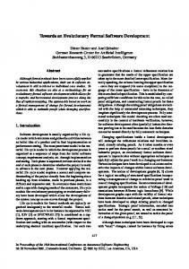
The formal testing method is an approach to find program errors with respect to the formal specification of the tested application: program behaviors are compared to those required by the specification. It is usually decomposed into the following three phases: (i) a test selection phase, in which some tests that express properties of the specification are generated, (ii) a test execution phase, in which the tests are executed and the results of the execution collected, and (iii) a test satisfaction phase, in which the results obtained during the test execution phase are compared to the expected results. This last phase is commonly performed through the help of an oracle [Weyuker 80a]. The formal testing method presented in this thesis is an adaptation to object-oriented software of the BGM method, developed by Bernot, Gaudel and Marre [Bernot 91b] for testing data types from algebraic specifications. The essence of the BGM method is to reduce the exhaustive test set into a finite and pertinent test set by applying hypotheses to the program behavior. The formal testing process is illustrated in figure 1.

Does the program satisfy its specification?

H0

Exhaustive test set T0

...

...

Application of

Hi

Ti

hypotheses to

Reduction

Hj

Tj

of the test set

...

...

H

T

the program

Test Selection

Test Requirement

Test Procedure

Test Execution Program Correction

Test Satisfaction

Yes — No — Inconclusive

Fig. 1. Formal testing process

16

Test Interpretation (Oracle)

Introduction

1.2 Contribution In this thesis, we present a method and a tool for test set selection, dedicated to object-oriented applications and based on formal specifications. The main contributions of this work are the following: • A theory of formal testing dedicated to object-oriented software We propose a theory of formal testing for object-oriented applications. This is a generalization of the BGM theory to systems where the specifications and the test sets can be expressed using different formalisms: a specification language well adapted to the expression of system properties from the specifier’s point of view, and a test language well adapted to the description of test sets from the tester’s point of view. Specifications are written in CO-OPN. Test sets are expressed using a very simple temporal logic, HML (Hennessy-Milner Logic), whose logic formulas can be executed by a program. We justify the choice of these formalisms, and establish that there exists a full agreement between the CO-OPN equivalence relationships and the HML equivalence relationships. We show that this full agreement between equivalence relationships leads to a full agreement between satisfaction relationships: the program satisfies its specification if and only if it satisfies the exhaustive test set derived from this specification. • A practical test set selection procedure We present a practical test selection process to reduce the (generally infinite) size of the exhaustive test set. The reduction is achieved by associating to each hypothesis applied to the program, a constraint on the test set. Our method proposes a set of elementary constraints: syntactic constraints on the structure of the tests and semantic constraints which allow to instantiate the test variables so as to cover the different classes of behaviors induced by the specification (i.e. subdomain decomposition). Elementary constraints can be combined to form complex constraints. Finally, the constraint system defined on the exhaustive test set is solved, and the solution leads to a pertinent test set of reasonable size. • A test format adapted to systems with states Thanks to the CO-OPN semantics, which allows to compute all the correct and incorrect behaviors induced by a specification, our method is able to test, on the one hand that a program does possess correct behaviors, and on the other hand that a program does not possess incorrect behaviors. An elementary test is defined as a couple . Formula is an HML formula composed of observable events of the specification. Result is a boolean value showing whether the expected result of the evaluation of Formula (from a given initial state) is true or false with respect to the specification. An advantage of this approach is to provide through the tests, an observational description (independent of the state notion) of valid and invalid implementations. • A new tool based on operational techniques for test set selection Our testing method exhibits the advantage of being formal, and thus allows a semi-automation of the test selection process. A new tool, called CO-OPNTEST, is presented in this thesis. This tool assists the tester during the construction of constraints to apply to the exhaustive test set; afterward it automatically generates a test set satisfying these

17

Introduction

constraints. The CO-OPNTEST architecture is composed of a PROLOG kernel and a Java graphical interface. The CO-OPNTEST kernel is based on the same technique as the LOFT 1 kernel which has a proven efficiency; it uses an equational resolution procedure which simulates narrowing by SLD-resolution, associating a Horn clause to each axiom of the specification. For that purpose, the formalisms involved in our test method (CO-OPN, HML, and a language of constraints CONSTRAINT) are translated into a logic program made of computational Horn clauses. Furthermore, the kernel includes additional control mechanisms for subdomain decomposition. The graphical interface allows a user-friendly definition of the test constraints. • A demonstration of the soundness of the approach via a case study of realistic size We present an application of CO-OPNTEST to a case study of realistic size: the control program of an existing industrial production cell [Lewerentz 95]. Test sets have been generated at both unit and integration level in a simple, rapid and efficient way. The design and execution of these tests have revealed errors in the design and implementation of the controller. CO-OPNTEST and its application to a significant example demonstrate the pertinence of our approach.

1.3 Document organization This document is organized as follows: • Chapter 2: Test Methods and Tools First, chapter 2 places formal testing in the verification and test context. Then, it considers the main object-oriented paradigms and their advantages and drawbacks for software testing. Finally, it presents several existing formal test methods together with their tools. • Chapter 3: The CO-OPN Object-Oriented Specification Language Our test method derives test sets from a formal specification language: CO-OPN (Concurrent Object-Oriented Petri Nets). Chapter 3 presents the syntax and the semantics of CO-OPN, as defined by Biberstein, Buchs and Guelfi. • Chapter 4: Theory of Formal Testing for Object-Oriented Software Chapter 4 presents our theory of formal testing for object-oriented software. It justifies the choice of CO-OPN as the specification formalism and of Hennessy-Milner temporal Logic (HML) as the test formalism, and then establishes that there exists a full agreement between these two formalisms. • Chapter 5: Practical Test Selection Chapter 5 presents the test selection process from a practical point of view. It proposes several reduction hypotheses together with their corresponding constraints2, studies the 1.

2.

18

The BGM method has led to the development of the LOFT tool (LOgic for Function and Testing, [Marre 91]) which semi-automatically generates test sets (algebraic formulas) from algebraic specifications. The complete language of constraints, CONSTRAINT, is given in annex E.

Introduction

subdomain decomposition problem, and finally shows how to transform a test set into a minimal test set free of redundant tests. • Chapter 6: Operational Techniques and Test Set Generation Tool: CO-OPNTEST First, chapter 6 presents the operational techniques for test set selection: translation of the formalisms involved in our test method (CO-OPN, HML, CONSTRAINT) into a logic program made of computational Horn clauses, the PROLOG resolution procedure, and control mechanisms for subdomain decomposition. Second, chapter 6 presents a new tool for test set selection based on the former techniques: CO-OPNTEST. • Chapter 7: Case Study: Production Cell Chapter 7 presents an application of CO-OPNTEST to a case study of realistic size: the control program of a production cell. This work is the result of a collaboration with Didier Buchs and Stéphane Barbey. In particular, earlier versions of chapters 4 and 5, related to the theory of testing, were conjointly written and can be found in [Barbey 96] and [Péraire 98a].

19

Introduction

20

Test Methods and Tools

C

H A P T E R

2

CHAPTER 2

TEST METHODS AND TOOLS

Testing is a verification technique to ensure that a program conforms to its specification. The goal of this chapter is to place testing in the general verification context, and to place formal testing in the test context. Furthermore, this chapter considers the main object-oriented paradigms and their advantages and drawbacks for software testing. It also presents several existing formal test methods together with their tools. To standardize the vocabulary used in this document, we start this chapter with some definitions taken from the IEEE Standard Glossary [IEEE 94]. Mistake

A human action that produces an incorrect result.

Error

A difference between a computed result and the specified or theoretical one.

Fault

A defect in a component which is the manifestation of an error.

Failure

The inability of a system to perform a required function within specified limits.

Consequently, an error is caused by a mistake and results in a fault that may produce a failure.

Mistake

Error

Fault

Failure

Several different definitions have been given for the word “testing”. In this document we adopt the one given by Myers [Myers 79]: Testing

The process of executing a program with the intent of finding errors.

21


Thus, testing is not the process of diagnosing the cause of errors, of correcting errors, or of proving the correctness of programs. The goal of testing is concentrated on finding program errors. However, testing has a side effect: the activity of designing tests early in the software development process allows to find errors in the design of the program. Furthermore, finding errors in both the program design and the implementation provides convincing evidence that there are no errors in the program. The structure of this chapter is the following. First, section 2.1 presents two orthogonal testing classifications. Second, section 2.2 considers the main characteristics of testing object-oriented software. Finally, section 2.3 presents several existing formal test methods together with their tools.

2.1 Testing classifications This section presents two orthogonal testing classifications. The first places the test in the software life-cycle. The second presents different test methods in the traditional verification taxonomy. All of the latter test methods can be used (individually or in conjunction) at each phase of the software life-cycle.

2.1.1 Testing in the software life-cycle

Abstraction level

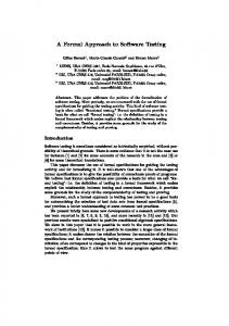
Several software life-cycle models are proposed in the literature, such as the “waterfall” model, the “V” model (see figure 2) and the “spiral” model. All of these models emphasize the importance of software testing at each development stage.

Acceptance and System testing

Analysis

Architectural design

Integration and Integration testing

Detailled design

Unit testing

Construction

Assembly and Verification Implementation

Sequencing

Verification link

Fig. 2. V model for software development

22

Time


In the “V” model, each construction phase (analysis, architectural design, detailed design) is reflected by a verification phase. The first verification phase is unit testing. During this phase, the tested software is divided into components, called basic units [Fiedler 89], that can be tested in isolation. Then, the basic units are integrated and integration testing is performed to scrutinize the interactions between the integrated units. Once the integration of all units is achieved, the system testing phase checks that the entire system meets its requirements. Unit, integration and system testing are performed using various testing strategies presented in the next section.

2.1.2 Test methods in the verification taxonomy In the traditional taxonomy [Laprie 95], verification techniques are divided into two families: static and dynamic methods (see figure 3). Dynamic methods involve the execution of the tested program, whereas static methods do not.

Verification

Static

Proof

Dynamic

Analysis

Program-based

Symbolic Execution

Test

Specificationbased ex: Formal

Deterministic Probabilistic Deterministic Probabilistic

Fig. 3. Classification of verification techniques

Static methods include proofs and static analysis. • Proving consists of stating the correctness of the program by establishing that its code satisfies theorems deduced from the specification. • Static analysis consists of analyzing the code of the program to verify that it satisfies implicit or explicit properties required by the specification. Static analysis can be either manual (e.g. code review) or automated (e.g. type checking, complexity measures).

23


Dynamic methods include symbolic execution and testing. • Symbolic execution is performed by executing tested programs with symbolic input values instead of concrete ones, and yields as results symbolic expressions corresponding to the outputs of the program. • Testing is performed by submitting a set of possible (concrete) inputs, called a test case, to the tested program, and comparing the computed result to the expected one. This comparison is performed manually or automatically by means of a program called an oracle. A test case exercises a particular aspect of the program. A set of test cases constitutes a test set. Since the exhaustive test set is usually infinite, its size must be reduced while retaining its pertinence. The goal is to select the smallest number of test cases that will detect the greatest number of errors in the tested program. This is usually achieved by sampling the input domain of the tested program to exercise the program with representative test cases only. Testing methods are divided into two families, according to the source from which test cases are selected: program-based testing and specification-based testing. • In program-based testing, also known as structural or white-box testing, test sets are derived from the code of the program. Tests cases are selected in order to cover a given coverage criterion (e.g. all instructions, all executable paths, all conditions) While this approach gives good results, it is insufficient. For instance, examining the code of the tested program is unlikely to detect that the program does not perform one of its desired tasks. Furthermore, using programs as models multiplies the work in the case of multiple implementations of one specification. In contrast, specification-based testing is efficient in this case. • In specification-based testing, also known as functional or black-box testing, test sets are derived from the specification of the tested application, apart from the program. The criterion of correctness is the specification of the tested application: program behaviors are compared to those required by the specification. The goal is to select test sets that cover each property described by the specification. Specifications can be either informal, semi-formal or formal. In the informal case, the specification is written in natural language. Test sets are selected manually for each functionality described by the specification. In the semi-formal case, test selection is guided by models of semi-formal development methods. For instance, test sets can be derived from the analysis and design models of the Fusion method [Coleman 94]. Partial automation of the test process is possible. In the formal case, specification-based testing is called formal testing. Thanks to mathematical notations and rules, the test selection process can be automated. Furthermore, this approach has the advantage of guaranteeing a good coverage of the specification properties. In addition to our formal language of choice, CO-OPN, which is described in detail in chapter 3, the references [Ehrich 91][Dodani 95], and [Guelfi 97] give an overview of various formal specification languages for object-oriented systems. Several experiments have been performed in testing using formal specifications. A good summary of the state of the art can be found in [Gaudel 95].

24


Specification-based testing is especially well-suited for testing object-oriented software, because it allows the reuse of test sets in the case of classes with multiple implementations. However, it is not sufficient to detect when the software performs undesirable tasks that are not contained in the specification. Program-based testing and specification-based testing are complementary techniques; the errors caught with one technique are not necessarily easily detected with the other. Their relationship is shown in figure 4, which is inspired by [Roper 94].

Unexpected additions detected by program-based tests

Program 1 (incorrect) Specification-based

Omissions detected by specification-based tests

Program-based tests 1

Specification tests (for both programs) Program 2 (correct)

Program-based tests 2

Fig. 4. Relationship between specification-based and program-based testing techniques

Both program-based testing and specification-based testing can be divided into two groups, according to the way test cases are selected: deterministic testing and what we call probabilistic testing. • Testing is deterministic when test cases are determined only according to a selective sampling criterion. • Testing is probabilistic when test cases are selected randomly, either on a uniform profile of the entry domain (random testing) or according to a probabilistic distribution (statistical testing) [Thévenod-Fosse 95]. Random test selection is easy, inexpensive and can give good results. However, this method is generally considered weak, because random test cases generally do not give a good coverage of the input domain. However, statistical testing does not have this flaw. Deterministic specification-based testing and statistical testing have been compared in [Marre 92] and have shown similar results. Since statistical testing is outside the scope of this work, we will not elaborate on this issue for object-oriented software. Interested readers can refer to [Thévenod-Fosse 97].

25


For the different test methods presented in this section, the quality of a test set, i.e. its power to reveal errors, must be measured by appropriate techniques [Binder 96]. Quality may be analyzed by techniques such as program mutation. In this analysis, faults are injected into a program, and the quality of the test sets is defined as a measure of the number of faults detected. For object-oriented software, this technique could be used if an appropriate mutation principle were defined. However, to our knowledge, no such mutation principle has yet been proposed. To conclude, it is important to note that an efficient verification strategy must adequately combine the use of the different static and dynamic verification techniques proposed in this section. These techniques must be used at each stage of the software development process.

2.2 Testing object-oriented software As stated in the introduction, object-oriented methods structure the software around objects and not around actions. A system is composed of a collection of connected objects. The main object-oriented concepts are objects, classes of objects, and inheritance between classes. This section presents the main object-oriented paradigms and their advantages and drawbacks for software testing. This section is gathered from a complete and detailed presentation on the subject which can be found in [Barbey 97]. A good survey of testing object-oriented software is presented in [Binder 94]. First, a major advantage of object-oriented programming could be that it is a unifying paradigm: in pure object-oriented programming languages, such as Smalltalk, everything is an object, and all statements and communications are stated with messages. However, many major object-oriented programming languages, such as Ada 95, C++, Eiffel and Java, are of a hybrid fashion; they include values and control structures found in structured programming languages, such as while, repeat and loop statements. Thus, they combine the sources of errors inherent to both programming styles.

2.2.1 Objects The main constituents of an object-oriented system are objects. An object is usually made up of three elements: a state, methods and an identity. • The state of an object consists of a set of attributes. In pure object-oriented systems, which do not admit entities other than objects, the attributes are objects. In hybrid object-oriented models, which also admit entities without identity such as natural numbers or booleans, the attributes can also be values. A state is encapsulated: it can only be observed or modified by means of the object methods. The presence of an encapsulated state is a benefit for testing object-oriented software, because it reduces the dispersal of information and defines an interface that determines the actions that can be performed on the object.

26


However, several programming languages, such as C++, Ada 95, Smalltalk and Eiffel, support mechanisms to break the encapsulation. Furthermore, the state of an object does not only include its local attributes. The attributes of connected objects must also be taken into account. Indeed, the behavior of a method may not only be influenced by the local state of the object on which it is applied, but also by those of connected objects. Consequently, an oracle that limits its observation to one object in order to test its methods may not be satisfactory. Furthermore, an oracle based on direct observation of states may be difficult to implement. It is therefore better to base the oracle on an external observation of the behavior. • The methods of an object are the subprograms which represent its behavior and can observe or modify its state. An advantage of methods for testing is that they are bound to a type, and thus that their context may be identified. Another advantage is that they are usually short. Wilde and Huit [Wilde 92] have collected data on three object-oriented systems and found that more than fifty percent of methods consist of one or two statements (C++) or four lines (Smalltalk). The drawback is that it is difficult to test a method individually. Generally, a method can only be tested through an object of a class. The context in which a method is executed is not only defined by its possible parameters, but also by the state of the object by which it is invoked and generally by the state of connected objects. • The identity allows identifying an object independently of its state. The management of object identity is generally part of the run-time environment of the system, and can be considered correct. The set of all attributes and all methods of an object is called its features, whereas the properties of an object denote both its features and its other characteristics, such as its implementation and the description of its semantics (by assertions, axioms, etc.).

2.2.2 Classes A class is a typed modular template from which objects are instantiated. It has two functions. • First, a class is a type. It is a means of classifying objects with similar properties. Each class represents the notion of a set of similar objects, i.e. of objects sharing a common structure and behavior. Associated with each class is a predicate that defines the criterion for class membership. • Second, a class is a module. A class encapsulates the features of its instances and can hide the data structures and other implementation details that should not be available outside of the class. The non-hidden features form the interface of the class. They are usually methods only. Therefore programmers can manipulate objects by invoking only these public methods and do not have to give special attention to the data representation of the class. This separation between interface and implementation is very important: a single specification can lead to multiple implementations. Since classes encapsulate a complete abstraction, they are easily isolated and can be reused in many applications.

27


Modularity simplifies testing because the determination of the components to be tested becomes easier, depending on the level of interconnection of the classes. Many authors consider the class to be the basic unit of test [Binder 94]. Some classes, such as abstract and generic classes, cannot be tested, because they do not contain enough information. Therefore, testing can only be performed on instantiations (for generic classes), or on concrete descendants (for abstract classes).

2.2.3 Inheritance Inheritance is a mechanism that allows a class, called the descendant class, to inherit features from one (single inheritance) or many (multiple inheritance) classes, called its parent classes. The descendant class can then be refined by modifying or removing the inherited methods, or by adding new properties. Inheritance is the prevailing mechanism in object-oriented programming languages for providing the subclassing relationship. Since the descendant class is obtained by refinement of its parent class, it seems natural to assume that a parent class that has been tested can be reused without any further retesting of the inherited properties. This intuition is however proved false in [Perry 90]: some of the inherited properties need retesting in the context of the descendant class. Furthermore, inheritance breaks encapsulation: the descendant class has access to the features of its parent class, and can modify them. Although encapsulation builds a wall between the class and its clients, it does not prevent the descendant class from changing the features of its parent class. Therefore, it is difficult to take advantage of completed testing of the parent class to test the descendant class. Nevertheless, to avoid retesting the entire set of inherited properties, it may be possible to select the minimal set of properties which are distinct in the parent and the descendant. Thus, only these properties need to be retested.

2.2.4 Polymorphism In addition to objects, classes, and inheritance, most object-oriented methodologies offer another important capability: polymorphism. Polymorphism is the possibility for a single name to denote different kinds of entities. Polymorphism can affect the correctness of a program and cause trouble during testing. For instance, it brings undecidability to program-based testing. Since polymorphic names can denote objects of different classes, it is impossible, when invoking a method on a polymorphic reference, to predict before run-time which code is about to be executed, i.e. whether the parent or a descendant implementation will be selected.

2.2.5 Summary Table 1 summarizes the advantages and the drawbacks of object-oriented paradigms for software testing.

28


Advantages • Object-oriented paradigms unify language constructs.

•

• • •

•

Drawbacks • Most object-oriented languages are hybrid and use structured statements and identity-less values. Objects Encapsulation reduces the dispersal of • Encapsulated states are not observable. information and defines an interface. • States depend on connected objects. • Objects of the same class may share a common state. • Encapsulation can be broken. Methods are bound to types. • Methods cannot be tested individually. Methods have few statements. Classes Modularity allows to determine test • Abstract and generic classes cannot be components. tested. Inheritance Capitalizing on inheritance can reduce • The part that needs no retesting is the number of tests for descendant difficult to determine. classes. • Inheritance breaks encapsulation. Polymorphism • No simple static analysis can be performed because of run-time binding. Table 1: Advantages and drawbacks of object-oriented paradigms for testing

2.3 Test methods and tools This section presents several existing formal test methods together with their tools. • The BGM method [Bernot 91b] and the LOFT tool [Marre 91] based on algebraic specifications. • The ASTOOT method and tools [Doong 94] based on object-oriented algebraic specifications (LOBAS). • The BULL method and tool [Dick 93] based on state-based specifications (VDM). • The TGV method and tool [Fernandez 96a] based on protocol specifications (SDL, LOTOS). These methods have been chosen so as to cover different types of formal specifications (algebraic, object-oriented, state-based, protocol) and because they present interesting features in terms of test selection strategies and tools.

29


2.3.1 The BGM method and the LOFT tool The BGM method has been developed at the LRI-CNRS (Laboratoire de Recherche en Informatique, University of Paris-Sud, Orsay, France) by Bernot, Gaudel and Marre. Complete presentations of the approach can be found in [Bernot 91b] and [Marre 91]. The method is based on the theory of testing presented in [Bougé 86] and [Bernot 91a]. • Goal The BGM method aims to test data types from algebraic specifications [Ehrig 85]. An example of an algebraic specification is given in figure 5 (CO-OPN ADT syntax). ADT Coordinates; Interface Use Naturals, Booleans; Sort coordinate; Generator : natural natural→ coordinate; Operations projection1: coordinate → natural; projection2: coordinate → natural; permutation:coordinate → coordinate; equivalence: coordinate coordinate → boolean; Body Axioms projection1 = x; projection2 = y; permutation = ; equivalence (,) = (x1 = x2) and (y1 = y2); Where x, y, x1, y1, x2, y2: natural; End Coordinates;

Fig. 5. Algebraic specification of the Abstract Data Type Coordinates

• Test unit and test coverage The approach aims to test operations (test units) of the specification. Since an operation is specified by means of axioms, the test selection process aims to cover all the axioms of each operation. • Test format Test cases derived from the algebraic specifications are algebraic equalities of the shape u = v, where u and v are ground terms well constructed from the specification interfaces. This kind of test allows to test the properties of operations. • Sampling techniques The method reduces the exhaustive test set into a finite and pertinent test set by applying reduction hypotheses to the program behavior. This hypotheses are of two kinds: uniformity and regularity. Uniformity hypotheses make the assumption that if an axiom, holding a variable, is satisfied for one instantiation of this variable, then it is satisfied for all possible instantiations of this variable.

30


Regularity hypotheses make the assumption that if an axiom, containing a term, is satisfied for all terms having a complexity less than or equal to a given bound, then it is satisfied for all terms whatever their complexity. Uniformity and regularity hypotheses can be combined in order to obtain more complex reduction hypotheses. Since uniformity hypotheses are very strong, they are usually not applied to the elements under test, but to the elements imported into the specification, which are assumed to be already tested. To the elements under test, regularity hypotheses are applied, as well as uniformity hypotheses combined with subdomain decomposition. Subdomain decomposition allows to instantiate variables of an axiom so as to cover the different classes of behaviors described by the specification. Subdomain decomposition is performed by unfolding the operations occurring in the axiom. This technique is illustrated with the decomposition of the axiom equivalence (,) = (x1 = x2) and (y1 = y2)

by unfolding of the operation and described by the following axioms: true true false false

and and and and

true false true false

= = = =

true, false, false, false.

This unfolding leads to the following four formulas: (x1 = x2) = true and (x1 = x2) = true and (x1 = x2) = false and (x1 = x2) = false and

(y1 = y2) = true (y1 = y2) = false (y1 = y2) = true (y1 = y2) = false

⇒ ⇒ ⇒ ⇒

equivalence (,) equivalence (,) equivalence (,) equivalence (,)

= = = =


The instantiation of the variables x1, y1, x2 and y2 by uniformity hypotheses leads, for instance, to the following four test cases: equivalence () equivalence () equivalence () equivalence ()

= = = =


A test set derived from the exhaustive test set with the preceding reduction hypotheses is valid (it rejects any incorrect program) and unbiased (it accepts any correct program) for a program satisfying these hypotheses. • Oracle The oracle is a decision procedure to verify that an implementation satisfies a test set. The oracle is based on equivalence relationships that compare the outputs of the execution of the test cases with the expected results derived from the specification; these elements are said to be observable. The problem is that the oracle is not always able to compare all the necessary elements to determine the success or failure of a test case; these elements are said to be non-observable. This problem is solved using oracle hypotheses. The oracle hypotheses stipulate that for any observable test case, the oracle is able to determine whether the test execution yields yes or no, i.e. that no test case execution remains inconclusive. Furthermore, they stipulate that for any non-observable test case, there exist observable contexts to transform it into observable test cases.

31


For instance, consider an oracle which is able to compare natural values with the operation =, and holds the operations projection1, projection2, and permutation, but which is not able to compare coordinates because it does not hold the operation equivalence. This oracle is not able to observe the test permutation = . However, this test can be observed using observable contexts: projection1 (permutation ) = projection1 (), projection2 (permutation ) = projection2 ().

In the past few years, many aspects of the BGM method have been enhanced to take into account exceptions [Gall 93] and bounded specifications [Arnould 97]. The BGM method has led to the development of the LOFT tool (LOgic for Function and Testing, [Marre 91]) which semi-automatically generates test sets (algebraic formulas) from algebraic specifications. • Operational techniques for test selection The LOFT kernel is an equational resolution procedure which simulates conditional narrowing by PROLOG SLD-resolution, associating a Horn clause to each axiom of the specification. Furthermore, it includes additional control mechanisms for subdomain decomposition. These techniques are presented in chapter 6. • User assistance LOFT proposes several PROLOG predicates (e.g. unfold_std, do_not_unfold) to assist the tester during the selection of hypotheses to reduce the exhaustive test set. The PROLOG queries are written via a text window. A Tcl/Tk graphical interface allows to define resolution parameters. Practical experiences at an industrial level, for example the application of LOFT to an automatic subway [Dauchy 93], have shown that this tool can be used successfully for complex problems.

2.3.2 The ASTOOT method and tools The ASTOOT (A Set of Tools for Object-Oriented Testing) method and tools have been developed by Frankl and Doong at the Polytechnic University of Brooklyn (New York, USA). Complete presentations of the approach and tools can be found in [Doong 93] and [Doong 94]. • Goal The ASTOOT method aims to test object-oriented programs from object-oriented algebraic specifications written in LOBAS [Doong 93]. • Test unit and test coverage The approach aims to test classes (test units) of the specification by focusing on method interactions. Since a method is specified by means of axioms, the test selection process aims to cover all the axioms of each method involved in an interaction.

32


• Test format Test cases are triplets (T, T’, tag) where T and T’ are sequences of method calls, and tag is a boolean value showing whether T is equivalent to T’ according to the specification. T is a sequence supplied by the user while T’ is a simplified sequence computed by the method. T and T’ are equivalent if the axioms of the specification can be used as rewrite rules to transform T into T’ (thus the specification must define a convergent rewriting system). A sequence of method calls has the following limitations: - methods have no side effects on their parameters, - observers have no side effects, - observers can only appear as the last method of a trace, - when a sequence is passed as a parameter to a method, it must not contain any observers. These limitations permit the construction of an oracle and thus ensure the program testability. However, this format does not always reflect the reality of object-oriented programs, for instance by neglecting the potential side effects of observers. • Sampling techniques The test set selection is based on original sequences T supplied by the user. These original sequences are selected either by hand or randomly; this is a limitation with regard to test quality. Then, using the axioms of the specification, each sequence T is rewritten into several simplified sequences. This simplification leads to test cases such as (T, T’, equivalent) or (T, T”, not-equivalent). This simplification is performed by a case analysis of the axioms. • Oracle The method requires that the class under test Class and each class that is returned by a function of Class include an equivalence function that approximates an observational equivalence between objects (for instance, two FIFO queues may be considered equivalent if they have the same number of elements). The equivalence function is based on a detailed knowledge of how data is represented and manipulated in the class body. Thus, for a test case (T, T’, tag), the oracle checks whether the result of the equivalence function, applied to the objects returned by T and T’, is equal to tag. This approach has the advantage of simplifying the oracle problem to a trivial boolean comparison. The ASTOOT approach is embodied in a testing system which includes a test selection tool and a test execution tool. • Test selection tool The test selection tool translates the axioms of the algebraic specification, as well as the original sequences T supplied by the user, into an internal representation (ADT tree). This internal representation forms a rewriting system which allows to automatically rewrite T in several equivalent or non-equivalent sequences, and thus to generate test cases. Each test case is generated along with a set of constraints that must be solved manually in order to instantiate the remaining variables in the sequences. • Test execution tool A driver generator takes as input the interface specifications of the class under test and of some related classes, and outputs a test driver (a class in the implementation language).

33


This test driver, when executed, reads test cases, checks their syntax, executes them by sending sequences to objects of appropriate types, and checks the results by using equivalence functions to compare the objects and by checking whether the values returned by the functions agree with the corresponding tags. The current version of ASTOOT is targeted at the Eiffel programming language [Meyer 92], but could be suited for other languages.

2.3.3 The BULL method and tool The BULL method has been developed by Dick and Faivre at the Bull Corporate Research Center (Les Clayes-sous-Bois, France). A complete presentation of the approach can be found in [Dick 93]. • Goal The BULL method aims to generate test cases from state-based specifications written in VDM [Dawes 91]. • Test unit and test coverage The approach aims to test state components (test units) of the specification by focusing on operation sequences. For this purpose, a Finite State Automaton (FSA) is built for each state component, using the specification of the operations (each operation describes a state modification). Thus, the test selection process aims to cover all the FSA paths. • Test format Test cases derived from VDM specifications are sequences of operations of the interface, called test suites. • Sampling techniques The test selection process starts with a partition analysis of individual operations. The mathematical description of each operation is reduced to a Disjunctive Normal Form (DNF). This reduction creates a set of disjoint sub-operations. Each sub-operation yields a set of constraints which describe a single test domain. This reduction is equivalent to the unfolding technique proposed by the BGM method (see section 2.3.1). Furthermore, the recursive operations are unfolded a fixed number of times to ensure unfolding termination. This approach is similar to the use of reduction hypotheses in the BGM method. Second, a partition analysis of the system state is performed. This partition permits the construction of an FSA formed of transitions and states. FSA transitions are the sub-operations previously computed, while FSA states are disjoint classes of equivalent states (computed from the DNF of the sub-operation pre- and post-conditions). Finally, test suites are formed such that they ensure a certain coverage of the FSA paths. After the resolution of their combined constraints, test suites may contain remaining variables, which are randomly instantiated. This instantiation corresponds to the use of uniformity hypotheses in the BGM method.

34


• Oracle The oracle problem is not solved; no equivalence relationship between abstract FSA states and practical states is provided. The BULL method has led to the development of a tool described in [Dick 92], which semi-automatically generates test suites from VDM specifications. This tool is included in the VDM toolbox. • Operational techniques for test selection The partition analysis of individual operations is automated. Reduction to DNFs is performed in PROLOG. The formulas thus obtained are simplified using inference rules based on first order calculus. However, the construction of the FSAs by partition analysis is not automated. • User assistance The tool assists the user during the composition for test suites, and then solves their combined constraints. However, since VDM is based on a semi-decidable logic, it is not always possible to generate solutions to constraint systems. While dedicated to VDM specifications, the BULL method could be suited for other state-based specification languages. A similar method based on Z [Spivey 92] has been proposed by Hoercher and Peleska [Hoercher 94]. Finally, we can mention other state-based testing approaches, such as the Turner and Robson method based on sequential machines and described in [Turner 92], or the McGregor method based on finite state machines and presented in [McGregor 94].

2.3.4 The TGV method and tool The TGV (Test Generation using Verification techniques) method has been developed at INRIA (Institut National de Recherche en Informatique et en Automatique, Rennes, France) by Fernandez, Jard, Jéron, Nedelka and Viho. Complete presentations of the approach can be found in [Fernandez 96a] and [Fernandez 96b]. • Goal The TGV method aims to generate test cases from protocol specifications written in SDL (Specification and Description Language, [Belina 89]) or in LOTOS [Bolognesi 87]. The semantics of an SDL or LOTOS specification is expressed as Input-Output Labelled Transition Systems (IOLTS). • Test unit and test coverage The approach aims to test protocol entities (test units) of the specification by focusing on sequences of interactions (input and output messages) between the entity and its environment simulated by a tester, which is also the test driver. Since the sequences of interactions are specified with an IOLTS, the test selection process aims to cover all the IOLTS paths. • Test format A test case is derived from two elements: the specification of the entity and a test purpose.

35


A test purpose defines a sequence of interactions that one wants to test, and a set of constraints that must be applied to the implementation before testing. The behavioral part of the test purpose is also specified by an IOLTS in which transitions are labelled with interactions. This IOLTS is an abstraction of that of the protocol specification. A test case is derived from the specification and test purpose if and only if both agree with a consistency relation. This is a weak notion of satisfaction meaning that at least one sequence of the IOLTS of the specification is accepted by the IOLTS of the test purpose. A test case is obtained by computing the synchronous product of the IOLTS of the specification with the IOLTS of the test purpose: a transition is firable in the product if either it is firable in the two components or if it is firable only in the specification. The result is an acyclic test graph labelled with input and output observable messages, verdicts (partial success, total success, failure, inconclusive) and timers to detect deadlocks or infinite loops. The test graph is then translated into a tree in standard notation (TTCN: Tree and Tabular Combined Notation, [OSI 92]). This tree, in which each branch describes a sequence of interactions between the protocol and the tester, is the test case. • Sampling techniques The method is more concerned with control (sequencing of actions) then with data. The variables are thus generally instantiated in the exhaustive way. To obtain a test graph of reasonable size, the test purpose introduces a set of constraints that must be applied to the implementation before testing (ex: forbidden actions). Furthermore, some hypotheses are introduced. - Bounded fairness hypothesis: a bounded number of executions of a non-deterministic implementation will show all its behaviors. - Reasonable environment hypothesis: each time the environment sends a message to the network, it waits for stabilization. This means that no new message can be sent by the environment until it receives all specified outputs of the protocol. This hypothesis allows to avoid concurrency between inputs and outputs by limiting the crossing messages. The test case construction ensures that, modulo these hypotheses, a test case rejects any incorrect program and accepts any correct program. • Oracle A notion of conformance of an implementation with respect to the specification is introduced. The conformance relation states that outputs of the environment which are not accepted by the specification may be accepted by the implementation, but inputs produced by the implementation must be also produced by the specification. The tester exercises the implementation with input messages following branches of test cases. It compares output messages of the implementation with test verdicts. The TGV method has led to the development of a tool which automatically generates test cases from SDL or LOTOS specifications and from test purposes that must be defined manually. This tool is included in the CADP toolbox [Fernandez 92a].

36


• Operational techniques for test selection The TGV kernel is an extension of an on-the-fly verification algorithm presented in [Fernandez 92b]. It is based on depth-first traversal of the synchronous product of the IOLTS of the specification with the IOLTS of the test purpose. During the traversal, the consistency relation is checked. If the relation is satisfied, an acyclic test graph is generated and labelled with verdicts and timers. The test graph is then unfolded in a tree in the TTCN format. The TGV tool has been successfully used to generate test cases for an industrial protocol, the DREX protocol. This experiment has shown the effectiveness of the approach for complex protocols.

2.3.5 Summary Table 2 on page 38 presents a summary of this section.

37


BGM-LOFT

ASTOOT

BULL

TGV

Algebraic specifications

Object-oriented algebraic specifications LOBAS

State-based specifications VDM (FSA)

Protocol specifications SDL - LOTOS (IOLTS)

Test unit

Operation

Class (method in interaction)

State component (sequences of operations)

Protocol entity (sequences of input and output messages)

Test coverage

Axioms

Axioms

FSA paths

IOLTS paths

Test format

Equality

triplet (trace 1, trace 2, equivalence between traces)

Sequence of operations

TTCN tree (tree branches are sequences of input and output messages)

Sampling techniques

Reduction hypotheses

Random

Partition analysis based on DNF reduction

Constraints and hypotheses

Oracle

Equivalence relationships with observable contexts

Equivalence functions

—

Conformance relation (external observation of the protocol behavior)

Operational techniques

PROLOG SLD-resolution with control mechanisms

Rewriting based on ADT trees

DNF reduction using PROLOG, Simplification using inference rules

On-the-fly algorithm for depth-first traversal of graphs product

User Assistance

Selection of hypotheses (PROLOG predicates), User-friendly interface for resolution parameters

—

Composition of test suites

—

Tool

Method

Model

Table 2: Main characteristics of four test methods and tools

38

The CO-OPN Object-Oriented Specification Language

C

H A P T E R

3

CHAPTER 3

THE CO-OPN OBJECT-ORIENTED SPECIFICATION LANGUAGE

The testing method presented in this document requires the use of a formally defined specification language. This language must have a syntax well adapted to the specification of object-oriented systems, and a semantics allowing to prove and deduce system properties. Furthermore, behaviors of the semantics must be automatically computed by operational techniques. Therefore we have chosen to use an object-oriented specification language which satisfies these criteria: CO-OPN (Concurrent Object-Oriented Petri Nets). This section describes the CO-OPN formalism. This presentation, based on [Biberstein 95a], [Barbey 97], [Hulaas 97] and [Buffo 97], does not cover all of the language, but only the parts which are relevant to this work. Interested readers will find the complete and formal definition of the language in [Biberstein 97a] or [Biberstein 97b]. The CO-OPN formalism is devoted to the specification of large and complex concurrent systems. The two underlying formalisms of CO-OPN are the algebraic specifications [Ehrig 85] and the Petri nets ([Brams 83a], [Brams 83b], [Proth 95]) which are combined in a more general model: algebraic nets [Reisig 91]. Algebraic specifications are used to describe the data structures and the functional aspects of the system, while Petri nets serve to model the behavioral and concurrency features. However, algebraic nets are not suitable to specify large and complex concurrent systems. This lack of structuring capabilities is compensated by the introduction of a complete set of object-oriented concepts: object, class, modularity, encapsulation, object identity, dynamic creation, inheritance, subtyping, substitution, genericity, etc. These features make the language suited to illustrate our theory of testing object-oriented software.

39


The structure of this chapter is the following. First, section 3.1 presents the CO-OPN object-oriented concepts. Second, section 3.2 introduces the CO-OPN object-oriented specification language using a small but significant example: a telephone system. Finally, section 3.3 and section 3.4 are a formal presentation of the syntax and the semantics of CO-OPN.

3.1 CO-OPN object-oriented concepts CO-OPN specifications are defined using different kinds of modules: abstract data types (ADT), objects and classes; CO-OPN is thus a hybrid object-oriented specification language. The modules are used to define sorts and their related operations. All the modules have a similar structure: in addition to a header which holds the module name and the information related to genericity or inheritance, each module has a public part, the interface which lists sorts and public operations, and a private part, the body which defines the properties of the operations. • ADT modules ADT modules contain data structure definitions. These data structures are defined with algebraic sorts and operations. Their behavior is defined by algebraic formulas and theorems. These sorts are used to describe passive entities, such as values of primitive sorts (e.g. boolean, integer, enumeration types) or purely functional sorts (e.g. stacks). Algebraic sorts are specified using hierarchical order-sorted algebraic specifications [Goguen 92]. Indeed, notions like subsorting, partial operations, polymorphism and overloading, which are required by CO-OPN, are well encompassed within the order-sorted algebra framework. • Object modules Object modules define a single instance of an object, using class’type sorts (later simply called types) and operations. The operations are the services provided by the object. Services are also called methods or events. Their behavior is defined by behavioral axioms. Object encapsulation. An object is an encapsulated entity (an encapsulated algebraic net) that holds an internal state (each place of the net stores a multi-set of algebraic values) and provides the outside with various services (parametrized transitions of the net). The only way to interact with an object is to request one of its services. The internal state is then protected against uncontrolled access. Object communication. Objects communicate with each other by means of services, i.e. by triggering one of their external events. There are three kinds of services: creation methods (which allow dynamic creation of a new object), methods (which provide changes of the state of an object, or allow the observation of this state) and destruction methods (which allow the destruction of objects). Interaction between objects is synchronous. When an object invokes a method on another object, it asks to be synchronized with the method of the object provider. The synchronization will only occur if the object provider can offer the service. The synchronization is specified by means of synchronization expressions that

40


appear in the axioms of the classes. Synchronization expressions may involve many partners, as well as synchronization operators of three kinds: sequence, simultaneity and alternative. Objects and concurrency. CO-OPN objects are not restricted to sequential processes. CO-OPN provides both inter- and intra-object concurrency, because the granularity of concurrency is associated with method invocation rather than with objects. Each object possesses its own behavior and concurrently evolves with other objects, and a set of method calls can be concurrently performed on the same object. Object identity. Each object has an identity, called an object identifier, that may be used as a reference. • Class modules Class modules are templates for objects; all the objects of one class have the same structure. They define types from which objects can be dynamically created. These types are used to describe active entities requiring dynamic creation, identity, concurrency, persistent state, etc. CO-OPN provides two relationships between classes: inheritance and subtyping (a relation similar to subtyping, called subsorting, can also hold between ADTs). Inheritance is the syntactic mechanism which allows reuse and refinement: a class may inherit all the features of another class and may also add services or change the description of already defined services. Subtyping addresses a semantic conformance relationship between types; it limits the enrichment to what is allowed by the strong substitution principle. A class instance of a subtype may substituted for a class instance of its supertype only if the whole system remains unchanged. This conformance relationship is based upon bisimulation between the semantics of the supertype and the semantics of the subtype restricted to the behavior of the supertype. A module can be effective (directly usable), abstract (it defines types for which no instances can be created), generic (it is parameterized by other modules), or parameter (it defines the properties of a module parameter in a generic module). A dependency graph can be built among the different modules of a specification. A module is said to be dependent on another module if the former imports the latter, if the former inherits from the latter, or if the latter is used as an actual generic parameter. A well-formed CO-OPN specification does not allow cycles in the dependency graph.

3.2 Introductory example: the telephone system To introduce CO-OPN, we present a small but significant example: a simplified telephone system. This example models the behavior of a telephone machine that can be used with a phonecard. Each phonecard includes an identification code that is also known to the user, and is requested by the telephone machine when the user tries to make a phone call and to pay with the card. The remaining balance is also stored on the card.

41


From this description, we can identify several entities such as the telephone, phonecard, pin-code, and money. Amongst these entities, several are objects, which have an identity that makes them discernible from other objects with the same state (telephone and phonecard), whereas other entities are merely values (pin-code and money). The state of an object phonecard consists of the amount of money available on the card, and of a pin-code. A phonecard provides services to withdraw money from the card, check the pin-code, or yield the balance of the remaining money on the card. The state of a telephone consists of the amount of money collected by the telephone, and a (possibly) connected phonecard. A telephone offers services to insert a card, eject it, buy communication time, etc. Several modules are encompassed in this system: • ADTs (Pin, Money, Booleans and Naturals), • classes (PhoneCard and Telephone).

Telephone

enter(p)

enter(p)

insert(c)

buy(m)

c, s

c, s

c, s

c, s c, s

c, s c, s

s

wait-for-pin create

idle

buy(m)

wait-for buy c, s+m c, s

s

withdraw (m)

c, s

eject

ready-to-eject get-pin (p) get-balance(b) b b

b-m

p

p

b

p

create (p) id Pin

Money

balance

PhoneCard

Fig. 6. The classes and their internal description and synchronizations

In figure 6, we give a partial representation of the classes, their synchronizations and their client relationships with abstract data types. This figure follows the following conventions: • The grey rectangles represent ADT modules. • The ellipses represent class modules, the inside of the ellipses representing what is encapsulated: • The solid black rectangles represent the methods. • The white rectangles correspond to the internal transitions. • The solid grey rectangles correspond to the creation methods. • The circles identify the places or the object attributes. • The solid arrows indicate the data flow. • The grey arrows indicate the synchronizations. • The dotted arrows indicate dependency on ADTs.

42


3.2.1 ADT modules In our example, the balance (ADT Money) as well as the personal identification number (ADT Pin) require no concurrency, and do not require a persistent state. They are modeled as abstract data types (see figure 7). The ADTs Booleans and Naturals are data types axiomatized as usual (see annex A.2. and annex A.3). Since the ADT Money is defined to model the balance, it seems natural to describe this type as a copy of the ADT Naturals. It inherits all the operations of Naturals, and changes the name of the sort natural into money. So the modules Naturals and Money are related by a subclassing relationship, but the types natural and money are not related by a subsort relationship. Thus no substitution is possible for these two types. The ADT Pin imports the ADT Boolean. Its signature consists of a sort, pin, and three operations: two generators to create new pins, and one function to compare two pins. The generator first-pin has no parameter and the generator new-pin has a post-fixed parameter of sort pin. .The function “=” is an in-fix operation, with two parameters of sort pin. ADT Pin; Interface Use Booleans; Sorts pin; Generators first-pin : → pin; new-pin _ : pin → pin; Operations _ = _ : pin pin → boolean; Body Axioms (new-pin (n) = new-pin (m)) = (n = m); (new-pin (n) = first-pin) = false; (first-pin = new-pin (m)) = false; (first-pin = first-pin) = true; Where n, m : pin; End Pin;

ADT Money; Inherit Naturals; Rename natural → money; End Money;

Fig. 7. The ADTs Pin and Money

The axioms of Pin define the algebraic conditions that hold between the various operations of the specification. All functions are totally defined. These axioms make use of two variables, n and m, of sort pin.

43


3.2.2 Class modules Figure 8 shows the textual description of the class PhoneCard (the graphical representation in figure 6 is equivalent to this textual representation). This module imports the ADT modules Pin and Money. It defines a type, phonecard, together with four exported methods. The first method, create, must be called to create a phonecard. It is given a parameter of type pin. The three other methods, get-pin, withdraw and get-balance provide services to get the pin-code (get-pin), to access the balance (get-balance), and to reduce it (withdraw). Since it is a throw-away card, it is not possible to reload it. The state of a phonecard is encapsulated in the body of the module. It includes the place balance, a multi-set of algebraic values of sort money, which stores the money still available on the card, and id, which stores the pin-code. For each new card, the balance is initialized to an initial marking in which the constant value 20 is assigned as the initial amount of money on the card. In the field Axioms, the behavior of the methods is given by Petri net causal relations. Since the places are independently accessed through the methods, concurrent access can be performed on the places id and balance. However, it is not possible to simultaneously read the balance and withdraw money, because get-balance and withdraw use the same critical resource balance. Class PhoneCard; Interface Use Pin, Money, Booleans; Type phonecard; Creation create _ : pin; Methods get-pin _ : pin; withdraw _ , get-balance _ : money; Body Places balance : money; id : pin; Initial balance 20; Axioms create (p) :: → id p; get-pin (p) :: id p → id p; get-balance (b) :: balance b → balance b; withdraw (m) :: (b ≥ m) = true ⇒ balance b → balance b - m; Where b, m: money; p: pin; End PhoneCard;

Fig. 8. Textual specification of the class PhoneCard

44


The creation method implicitly performs the initialization of a newly created object, and stores a pin-code in the place id. Get-pin returns the value of this place, assuming that the card has been created (and that the place id is not empty). Get-balance has the same behavior, but on the place balance, to return the amount of money still available on the phonecard. The method withdraw can only be fired if the amount of money available on the card is greater than the amount of money that the client wants to withdraw. These axioms make use of three variables of the imported sorts money and pin. We can imagine another kind of phonecard which allows reloading cards (see figure 9). Class ReloadablePhoneCard; Inherits PhoneCard; Rename phonecard → reloadablephonecard; Interface Use PhoneCard; Subtype reloadablephonecard < phonecard; Creation create _ : pin; Methods reload _ : money; Body Axioms create (p) :: → id p; reload (m) :: balance b → balance b +m; Where b, m: money; p: pin; End ReloadablePhoneCard;

Fig. 9. Textual specification of the class ReloadablePhoneCard

The class module ReloadablePhoneCard inherits from the class module PhoneCard, and renames the type phonecard in reloadablephonecard. These two types are related by a subtype relation, in the clause Subtype, which states that reloadablephonecard is a subtype of phonecard. This class provides two new methods. One is a method create which has the same semantics as the method create in the class PhoneCard, but must be defined since creation methods are not inherited. It also provides a method reload to increase the amount of money stored on the card. The class Telephone (figure 10) specifies the behavior of the automaton which accepts a card, waits for and checks a pin-code, and, as long as the pin-code is correct, reduces the balance of the card by a given amount corresponding to the price of a phone call. It imports three ADT modules: Pin, Money, and Booleans; and a class module, PhoneCard. A type, telephone, is defined inside Telephone, as well as a static instance of that type named cabin. Three public services are provided by this class. These services are methods corresponding to the methods insert, enter and buy, which can be activated sequentially. Since no creation method is provided, instances of that class can be dynamically created by invoking a implicit method named create, which will only do the initialization.

45


Class Telephone; Interface Use Pin, Money, PhoneCard, Booleans; Type telephone; Object cabin : telephone; Methods insert _ : phonecard; enter _ : pin; buy _ : money; Body Places idle : money; wait-for-pin: phonecard money; wait-for-buy: phonecard money; ready-to-eject: phonecard money; Initial idle 0; Transition eject; Axioms insert (c) :: idle s → wait-for-pin c s; enter (p) With c.get-pin (pp) :: (pp = p) = true ⇒ wait-for-pin c s → wait-for-buy c s; enter (p) With c.get-pin (pp) :: (pp = p) = false ⇒ wait-for-pin c s → ready-to-eject c s; buy (m) With c.get-balance (b) :: (m > b) = true ⇒ wait-for-buy c s → ready-to-eject c s; buy (m) With c.get-balance (b) .. c.withdraw (m) :: (m > b) = false ⇒ wait-for-buy c s → ready-to-eject c s+m; eject :: ready-to-eject c s → idle s; Where s, m, b: money; c: phonecard; p, pp : pin; End Telephone;

Fig. 10. Textual specification of the class Telephone

The places of the class are used to describe the state of the telephone. In this state lies the money already collected by the telephone, and, when the machine contains a card (i.e. either an instance of phonecard or of reloadablephonecard) a reference to this card. These places are also used to sequentialize the events that are possibly triggered. Besides the observable events defined in the interface, an invisible event, the internal transition eject, is defined in the body of the specification. It is automatically activated if an error occurs, or when the process is finished. Its effects are not directly observable, but correspond to the rejection of the card. The behavior of the telephone is defined through its behavioral axioms. The syntax of the behavioral axiom is Event [With SynchroExpression] :: [Condition] ⇒ Precondition → Postcondition

in which: • Event is an internal transition name or a method with term parameters.

46


• SynchroExpression is an optional synchronization expression allowing cooperation between objects: each event may request synchronization with the method of one or a group of partners using a synchronization expression. Three synchronization operators are defined: “//” for simultaneity, “..” for sequence, and “⊕” for alternative. • Condition is a condition on the algebraic values, expressed with a conjunction of equalities between algebraic terms. • Precondition and Postcondition correspond respectively to what is consumed and to what is produced in the different places within the net (in arcs and out arcs in the net). Event can occur if and only if Condition is satisfied, as well as Precondition (the resources can be consumed from the places of the module) and Postcondition (the resources can be produced in the places).

The class Telephone makes synchronization requests to the phonecard in two cases. The first is to check the pin-code when a phonecard is inserted in the telephone, and the second is when money must be withdrawn from the card to pay for a call. This second behavior is modeled by the following two axioms: buy (m) With c.get-balance (b) :: (m > b) = true ⇒ wait-for-buy c s → ready-to-eject c s; buy (m) With c.get-balance (b) .. c.withdraw (m) :: (m > b) = false ⇒ wait-for-buy c s → ready-to-eject c s+m;

In the last axiom, the telephone synchronizes itself twice in sequence with the phonecard. The first time is to get the balance, and, provided that the amount of money available on the card is sufficient to pay for the call, the second time is to withdraw the price of the call.

3.3 Syntax of CO-OPN The purpose of this section is to describe the concrete and abstract syntax of CO-OPN. Recall that a CO-OPN specification is composed of different kinds of modules: ADT modules, class modules and object modules. The ADT modules are used to describe the algebraic abstract data types involved in a CO-OPN specification, whereas the class modules correspond to the description of the objects that are obtained by instantiation. From the abstract syntax point of view, the object modules are class modules for which only one instantiation is created.

3.3.1 Abstract data types 3.3.1.1 ADT concrete syntax Each abstract data type module contains four sections (the keywords starting each section or clause are written in bold):

47


The header contains information to identify the module, along with inheritance and genericity information. This section is introduced by the keyword ADT, followed by the module name. An optional Inheritance clause, which defines the inherited modules, allows a finer selection of the inherited components (through the clauses Rename, Redefine and Undefine). Generic ADTs are prefixed by the keyword Generic, and the parameter module follows the identifier of the ADT (between parentheses). The Interface includes the information on the components of the module that are accessible to its clients. This section includes: a Use clause, which lists the modules used by the interface definition; a Sort clause, to declare the names of the sorts specified in the package; a Subsort clause, to specify the subsort relationships among sorts; and a list of operations, in two separate clauses: Generator and Operation. These operations are coupled with their profile in which the underscore character ‘_’ gives the position of the respective arguments. This mixed notation allows pre-fix, post-fix, in-fix and out-fix profiles. The Body section describes the local aspects of the module, such as the behavior of its operations, by means of axioms. Clauses Use, Sort, Subsort, Generator and Operation can be reiterated for private components. The Axiom clause allows the expression of the properties of operations by means of formulas, or axioms. Properties that are logical consequences of the axioms can be expressed in a Theorem clause. The formulas are mainly used as conditional positive equations: [ Id : ] [ Condition ⇒ ] Term-1 = Term-2

where Id is an optional identifier, Condition an optional condition to limit the validity of the axiom to a certain context, and (Term-1 = Term-2) is an equation in which Term-1 and Term-2 are terms well constructed from module interfaces. The variables used in the axioms or in the theorems clauses must be defined in a Where clause that follows the former clauses. The next section presents the ADT abstract syntax. 3.3.1.2 ADT abstract syntax The aim of this section is to give the formal definition of an ADT module, which consists of an ADT signature, a set of axioms, and some variables. Recall that algebraic sorts are specified using hierarchical order-sorted algebraic specifications [Goguen 92]. Notations Throughout this chapter, we consider a universe including the disjoint sets: S, F, M, P, V, O. These sets correspond respectively to the sets of all sorts, operations, methods, places, variables and static object names. S is made of the two disjoint sets SA and SC, the sets of sort names in algebraic specifications and of type names in classes. The “S-sorted” notation facilitates the subsequent development. An S-sorted set A is a family of sets indexed by S, and noted A = (As) s ∈ S. Given two S-Sorted sets A and B, an S-sorted function µ : A → B is a family of functions indexed by S denoted µ = (µs : As → Bs)s ∈ S.

48


The partial order ≤ ⊆ (S × S) is extended to strings of equal length in S* by: s1,..., sn ≤ s’1,..., s’n iff si ≤ s’i (1 ≤ i ≤ n). Similarly, ≤ is extended to pairs in (S* × S) by: (w, s) ≤ (w’, s’) iff w ≤ w’ and s ≤ s’. Function name f ∈ Fs 1 ... s n, s is denoted by f : s1,..., sn → s. Constant name f ∈ Fε, s is denoted by f : → s (ε being the empty string). Formally the signature of an ADT module consists of three elements of an algebraic data type: a set of sorts, a subsort relation, and some operations. Since the specifications are structured into modules, they can use elements that are not locally defined, i.e. defined outside the signature itself. Thus, the profiles of the operations as well as the subsort relations are defined over the set of all sort names SA and not only over the set of sorts defined in the module SA. Otherwise the signature is said to be complete. Definition 1. ADT signature, order-sorted signature, complete ADT signature The signature of an ADT (over S and F) is a triplet ΣA = 〈SA, ≤A, F〉 where • SA is a set of sort names of SA, • ≤A ⊆ (SA × SA) ∪ (SA × SA) is a partial order (partial subsort relation), • F = (Fw, s) w ∈ S*, s ∈ S is a (S* × S)-sorted set of function names of F. An order-sorted signature is a triplet Σ = 〈S, ≤, F〉 in which S ⊆ S, ≤ ⊆ S × S, and F is a (S* × S)-sorted function. A signature is said to be complete if it only uses locally defined elements.

◊

Some properties are required on order-sorted signatures such as monotonicity, regularity, and coherence for the well-definedness of term interpretation and the existence of quotient structures. Definition 2. Monotonicity, regularity, and coherence Let Σ = 〈S, ≤, F〉 be an order-sorted signature. Σ satisfies the monotonicity conditions iff f ∈ F w1, s1 ∩ F w2, s2 and w1 ≤ w2 imply s1 ≤ s2. Σ is regular iff Σ is monotonous and given f ∈ F w1, s and w0 ≤ w1 there is a least 〈 w, s 〉 ∈ S* × S such that w0 ≤ w and f ∈ Fw,s. Σ is coherent iff it is regular and each sort s has a maximum in S.

◊

More details about these properties are given in [23]. Inside ADT signatures, functions are divided into two groups, generators and operations. Definition 3. Generators and operations Inside F we can distinguish C and OP, respectively a finite set of constructors, also called generators, and a finite set of operations, sometimes called defined or derived operations. The sets C and OP are disjoint. Moreover we have F = C ∪ OP. ◊

49


At an abstract level, these two notions can be assimilated. The variables used in the axioms are said to form an S-Sorted variable set. Definition 4. S-sorted variable set Let Σ = 〈S, ≤, F〉 be a complete signature. An S-sorted set of Σ-variables is an S-indexed set X = (Xs) s ∈ S of disjoint subsets of X.◊ As usual, the properties of the operations of a signature are described by means of equations (more generally conditional positive equations) which consist of pair of terms. Definition 5. Set of all terms Let Σ = 〈S, ≤, F〉 be a complete order-sorted signature and X be an S-sorted variable set. The set of all terms over Σ and X is the least S-sorted set TΣ, X = ((TΣ, X)s)s ∈ S inductively defined as: • x ∈ (TΣ, X)s for all x ∈ Xs, • f ∈ (TΣ, X)s for all f : → s’ ∈ F such that s’ ≤ s, • f (t1, ..., tn) ∈ (TΣ, X)s for all f : s1, ..., sn → s’ such that s’ ≤ s and for all ti ∈ (TΣ, X)si (1 ≤ i ≤ n).

◊

Definition 6. Variables, groundness and linearity of terms Let Σ = 〈S, ≤, F〉 be a complete signature and X be an S-sorted variable set. Var (t) is the set of variables occurring in the term t ∈ (TΣ,X)s. When Var (t) = ∅, the term t is said to be ground. When each variable is present no more than once, t is said to be linear.

◊

Since we use order-sorted approach, i.e. with subsorting, both terms of an equation do not necessarily have comparable sorts, but their least sort must be in the same connected component, i.e. they must be related in the transitive symmetric closure of the subsort relation [Goguen 92]. Definition 7. Equation and positive conditional equation Let Σ = 〈S, ≤, F〉 be a complete signature and X be an S-sorted variable set. An equation is a pair 〈 t, t' 〉 of equally sorted terms: ∃ a sort s such that t, t' ∈ (TΣ,X)s. A positive conditional equation is an expression ◊ e1 ∧ ... ∧ en ⇒ e where e, ei (1 ≤ i ≤ n) are equations. Thus, the description of an ADT module consists of an ADT signature, which may use elements that are not locally defined, a set of axioms, and some variables.

50


Definition 8. ADT module Let Σ be a set of ADT signatures, and Ω be a set of Class interfaces (see definition 9) such that the global signature (see definition 15) ΣΣ,Ω = 〈S, ≤, F〉 is complete. An ADT module is a triplet ModAΣ, Ω = 〈ΣΑ, X, Φ〉 where: • ΣΑ is an ADT signature, • X = (Xs)s ∈ S is an S-sorted variable set of V, • Φ is a set of positive conditional equations (axioms) over ΣΣ,Ω and X.

◊

Note that, according to the above definition, an ADT module may define data structures of object identifiers because the variables and components of the profile of the operations can be of sort SC. 3.3.1.3 Relation between abstract and concrete syntax of an ADT The relation between abstract and concrete syntax of an ADT is shown in figure 11 with the example of an unbounded stack of integers.

3.3.2 Classes 3.3.2.1 Class concrete syntax Classes have a structure similar to ADTs. They also include three parts that play the same role but contain different information. The header starts with the keyword Class, followed by the identifier of the class. This keyword may be prefixed by the keyword Generic, as for ADT modules, or by the keyword Abstract, if the class is not aimed to be implemented, for example because its sole purpose is classification. In this case no instance of this class may be created. A clause Inherit can also appear in the header. In the Interface section, the clause Use declares all modules required for the class definition. The clause Type declares the name of the type of the instances of the class. The clause Object declares static instances of the class. The clause Method declares the services provided by the class. The clause Creation lists methods concerned with the dynamic creation of instances of the class. Similarly, the clause Destruction may appear to declare methods that deal with the deletion of objects. The section Body includes a Use clause, and some internal methods (in a Method clause) or spontaneous transitions declared under the Transition clause. The state of the objects is described in a clause Places, as a list of attributes. The clause Initial declares the initial marking or the static initializations of each instance of the class. Finally, the properties of the methods and internal transitions are described by means of behavioral axioms within the clause Axioms. Recall that the syntax of the behavioral axiom is Event [With SynchroExpression] :: [Condition] ⇒ Precondition → Postcondition

51


Adt Fifo; (: Specification of an unbounded stack of integers :) Interface Use Naturals, Booleans;

SA ≤A

Sort fifo, non_empty_fifo; Subsort non_empty_fifo < fifo; Generators empty : → fifo; push _ _ : natural fifo → non_empty_fifo;

F

Operations size _ : fifo → natural;

(: Return the size of the stack :)

pop _ : non_empty_fifo → fifo;

(: Remove the first element :)

ΣΑ

C

OP ModA

top _ : non_empty_fifo → natural; (: Return the first element :)

Body Axioms size empty = 0; size (push n f) = size f + 1;

Φ

pop (push n f ) = f; top (push n f) = n;

Where

X

f : fifo; n : natural; End Fifo;

Fig. 11. Relation between abstract and concrete syntax in the ADT Fifo

in which: • Event is an internal transition name or a method with term parameters. • SynchroExpression is an optional synchronization expression allowing cooperation between objects: each event may request synchronization with the method of one or a group of partners using a synchronization expression. Three synchronization operators are defined: “//” for simultaneity, “..” for sequence, and “⊕” for alternative. • Condition is a condition on the algebraic values, expressed with a conjunction of equalities between algebraic terms. • Precondition and Postcondition correspond respectively to what is consumed and to what is produced in the different places within the net (in arcs and out arcs in the net). Event can occur if and only if Condition is satisfied, as well as Precondition (the resources can be consumed from the places of the module) and Postcondition (the resources can be produced in the places).

The next section presents the class abstract syntax.

52


3.3.2.2 Class abstract syntax The aim of this section is to give the formal definition of a class module, which consists of a class interface, a set of places, an initial marking, a set of variables and a set of behavioral formulas. The class interface includes the type of class, a subtype relation with other types, the set of methods that corresponds to the services that this class offers, and the set of predefined instances of the class. Definition 9. Class interface A class interface (over S, M, and O) is a quadruplet ΩC = 〈{c}, ≤C, M, O〉 in which • c ∈ SC is the type name of the class module, • ≤C ⊆ ({c} × SC) ∪ (SC × {c}) is a partial order (partial subtype relation), • M = (Mc, w) c ∈ {c}, w ∈ S* is a finite ({c} × S*)-sorted set of method names of M, • O = (Oc) c ∈ Sc is a finite SC-sorted set of static object names of O.

◊

For a type to be a subtype of another type, the profile of its methods must follow the following contravariance condition: Definition 10. Contravariance condition A set of class interfaces Ω satisfies the contravariance condition iff for any class interface 〈{c}, ≤C, M, O〉 and 〈{c’}, ≤C’, M’, O’ 〉 in Ω, the following property holds: if c ≤∅,Ω c’ then for each method mc’ : s’1, ..., s’n in M’ there exists a method ◊ mc : s1, ..., sn in M such that s’i ≤ si (1 ≤ i ≤ n). Note that in the CO-OPN context, a method is a parameterized synchronization rather than a function. Therefore, the usual co-variance of the function co-domain does not appear in the previous definition. In the CO-OPN context, multi-sets are used for two purposes. The first is the need for representing values of the places, and the second is for the expression of concurrency in the semantics. A multi-set is a set which may contain many copies of the same element. A multi-set is represented by a function from the set of elements to naturals. For example, the multi-set [a,b,a,c] over the set {a,b,c,d} is represented by the function: f : a → 2, b → 1, c → 1, d → 0. Formally a multi-set over a set E is a mapping from E to IN . The set of all multi-sets over a set E is defined by the set of all functions [E] = { f | f : E → IN } equipped with the operations [_] (coercion to the single-element set), + (set union) and ∅ (empty set) defined as follows: [e]

[E ]

( e' )

1

=

0

if e = e' otherwise

for all e, e' ∈ E

( f + [ E ] g ) ( e ) = f (e) + g(e) for all f , g ∈ [ E ] and for all e ∈ E

53


∅[E] (e) = 0 for all e ∈ E Thus, to express terms over multi-sets, we define the multi-set extension of a signature. The multi-set extension of a given order-sorted signature consists of the signature, enriched for each sort, with the multi-set sort, the multi-set subsort relation, and the multi-set operations. Definition 11. Multi-set extension of a signature Let Σ = 〈S, ≤, F〉 be an order-sorted signature. The multi-set extension of Σ is [Σ] = 〈 S ∪

∪ {[s]} ,

s∈S

  ∅ [ s ] : → [ s ],  ≤∪ { 〈 [ s ], [ s′ ]〉 } , F ∪  [ _ ] [ s ] :s → [ s ], s, s′ ∈ S s ∈ S  [s] s ≤ s′  + : [ s ], [ s ] → [ s ]

∪

∪

    〉   

◊ Before defining behavioral axioms, recall that CO-OPN provides two different kinds of events, namely invisible events and observable events. Both of them can involve an optional synchronization expression. The invisible events describe hidden spontaneous reactions of an object to modifications of the system state; they correspond to the internal transitions and are denoted by τ in the abstract syntax (and not by a specific name as in the concrete syntax). The observable events correspond to the methods which are accessible outside the module. A synchronization expression allows the object to synchronize itself with partners. Three synchronization operators are provided: “//” for simultaneity, “..” for sequence, and “⊕” for alternative. The set of all events over a set of parameter values A, a set of methods M, a set of object identifiers O, and a set of types of class modules C is written as EA, M, O, C. Because this set is used for various purposes, a generic definition is proposed. Definition 12. Set of all events Let S = SA ∪ SC be a set of sorts such that SA ∈ SA and SC ∈ SC. Let us consider a set of parameter values A = (As)s ∈ S, a set of methods M = (Ms, w)s ∈ SC, w ∈ S*, a set of object identifiers O = (Os)s ∈ SC, and the set of types C ⊆ SC. Events Event of EA, M, O, C are built following this syntax: Event → Invisible | Invisible with Synchronization | Observable | Observable with Synchronization Invisible → self.τ Observable → self.m (a1, .., an) | Observable SynchronizationOperator Observable Synchronization → o.m (a1, .., an) | o.create | o.destroy | Synchronization SynchronizationOperator Synchronization SynchronizationOperator → .. | // | ⊕ where s ∈ SC, si and s’i ∈ S (1 ≤ i ≤ n), a1 ... an ∈ As1, ×...× Asn, m ∈ Ms, s’1 ... s’n, o ∈ Os, ◊ c ∈ C, self ∈ Oc and such that si ≤ s’i .

54


For example, the observable event o.m (a1, a2) with o1.m1 (a1) // o2.m2 represents the simultaneous synchronization of the method m of an object o with both the methods m1 and m2 of two objects o1 and o2. Now the definition of the behavioral axioms is presented. The behavioral axioms are used to describe the properties of observable and invisible events (respectively, methods and internal transitions). Definition 13. Behavioral axioms Let Σ = 〈S, ≤, F〉 be a complete order-sorted signature such that S = SA ∪ SC (SA ∈ SA and SC ∈ SC). For a given (SC × S*)-sorted set of methods M, a set of object identifiers O, an S-sorted set of places P, a set of types C ⊆ SC, and an S-sorted set of variables X = XA ∪ XC where XA and XC are, respectively, an SA-sorted and an SC-sorted variable set. A behavioral axiom is a quadruplet 〈Event, Condition, Precondition, Postcondition〉 also denoted by the expression Event :: Condition ⇒ Precondition → Postcondition where • Event ∈ E (TΣ, X), M, O, C,

• Condition is a conjunction of equations over Σ and X, • Precondition = (Prep) p ∈P is a family of terms over ([Σ], X) indexed by P s.t. (∀s ∈ S) (∀p ∈ Ps) (Prep ∈ (T[Σ], X)[s]), • Postcondition = (Postp) p ∈P is a family of terms over ([Σ], X) indexed by P s.t. (∀s ∈ S) (∀p ∈ Ps) (Postp ∈ (T[Σ], X)[s]). ◊ Consequently, a class module can be defined by its interface, a state represented as places together with their initial values, behavioral axioms that define the properties of its methods and internal transitions, and variables used in these definitions. Definition 14. Class module Let Σ be a set of ADT signatures, and Ω be a set of class interfaces such that the global signature ΣΣ,Ω = 〈S, ≤, F〉 (see definition 15) is complete. A class module is a quintuplet ModCΣ,Ω = 〈ΩC, P, I, X, Ψ〉 in which: • ΩC = 〈{c}, ≤C, M, O〉 is a class interface, • P = (Ps) s ∈ S is a finite S-sorted set of place names of P, • I = (Ip) p ∈ P is an initial marking, a family of terms indexed by P such that

55


(∀s ∈ S) (∀p ∈ Ps) (Ip ∈ (T[Σ], X)[s]), • X = (Xs) s ∈ S is an S-sorted set of variables of V, • Ψ is a set of behavioral axioms.

◊

Note that the places and variables, as well as the profile of the methods, can be of sorts SC; thus the objects are able to store and exchange object identifiers. 3.3.2.3 Relation between abstract and concrete syntax of a class The relation between the abstract and concrete syntax of a class is shown in figure 12 with the telephone example. Class Telephone; Interface Use SuperTelephone; Type telephone;

{c}

Subtype telephone < supertelephone;

≤C O

Object cabin : telephone;

ΩC

Methods insert _ : phonecard; enter _ : pin; buy _ : money;

M

Body Places idle : money; wait-for-pin: phonecard money; wait-for-buy: phonecard money; ready-to-eject: phonecard money; Initial idle 0; Transition eject;

P

I τ

Axioms insert (c): idle s → wait-for-pin c s; (pp = p) = true ⇒ enter (p) With c.get-pin (pp): wait-for-pin c s → wait-for-buy c s; (pp = p) = false ⇒ enter (p) With c.get-pin (pp): wait-for-pin c s → ready-to-eject c s;

Ψ

(m > b) = true ⇒ buy (m) With c.get-balance (b): wait-for-buy c s → ready-to-eject c s; (m > b) = false ⇒ buy (m) With c.get-balance (b) .. c.withdraw (m): wait-for-buy c s → ready-to-eject c s+m; eject: ready-to-eject c s → idle s; Where s, m, b: money; c: phonecard; p, pp : pin;

X

End Telephone;

Fig. 12. Relation between abstract and concrete syntax in the class Telephone

56

Mod C


3.3.3 Syntax of a specification Given the previous definitions, it is possible to define the global signature and the global interface of a CO-OPN specification, and finally the CO-OPN specification itself. Definition 15. Global subsort/subtype relationship, signature and global interface Let Σ = (ΣAi)1 ≤ i ≤ n be a set of ADT signatures, and Ω = (ΩCj)1 ≤ j ≤ m be a set of class interfaces such that ΣAi = 〈SAi, ≤Ai, Fi〉 and ΩCj = 〈{cj}, ≤Cj, Mj, Oj〉. The global subsort/subtype relationship over Σ and Ω noted ≤Σ, Ω is: ≤ Σ, Ω = 〈

∪

1≤i≤n

≤ iA ∪

∪

1≤ j≤m

≤ Cj 〉 *

The global signature over Σ and Ω noted ΣΣ, Ω is: Σ

Σ ,Ω

= 〈

∪S

1≤i≤n

A i ∪

∪

1≤ j≤m

{c j}, ≤

Σ, Ω

,

∪F

1≤i≤n

i ∪

∪

F

∪

Oj 〉

1≤ j≤m

Ω Cj

〉

The global interface over Ω is: Ω

Ω

= 〈

∪

1≤ j≤m

{c j} ,

 

∪

1≤ j≤m

 ≤C j *,

∪

1≤ j≤m

Mj ,

1≤ j≤m

◊ Definition 16. CO-OPN specification Let Σ be a set of ADT signatures and Ω be a set of class interfaces such that the global signature ΣΣ,Ω is complete and coherent, and such that ΩΩ satisfies the contravariance condition. A CO-OPN specification consists of a set of ADT and class modules: Spec Σ,Ω = {(Mod

A ) Σ,Ω i

| 1 ≤ i ≤ n} ∪ {(Mod

C ) Σ,Ω j

| 1 ≤ j ≤ m}.

A CO-OPN specification SpecΣ,Ω is denoted by Spec and the global subsort/subtype relation ≤Σ,Ω by ≤ when Σ and Ω are, respectively, included in the global signature and in the global interface of the specification. In this case the specification is said to be complete. ◊ From a specification Spec, two dependency graphs can be constructed. The first consists of the dependencies which concern the algebraic part of the specification, i.e. between the various ADT signatures. The second dependency graph corresponds to the client-ship relationship between the class modules. A CO-OPN specification is said to be well-formed if there is no cycle in its dependency graphs.

57


3.3.4 Summary of the syntax of CO-OPN A summary of the syntax of CO-OPN, together with the symbols used for its different components, are given in table 3. A

Class

Mod

C

Module

ADT

Mod

Signature

signature

Σ

A

interface

ΩC

Sort/Type

algebraic sorts

S

A

class type

{c}

Hierarchy

subsort relation

≤

A

subtype relation

Services

operations (generators and functions)

F

Static instances

≤

C

methods (public and private)

M

—

objects

O

State

—

places

P

Initial State

—

initial markings

I

Reaction

—

internal transitions

τ

Specification of behavior

algebraic formula (axioms and definedness formula)

behavioral formula

Ψ

defined with

algebraic terms

Body

using variables

Φ

events X

X

Table 3: Summary of the syntax of CO-OPN

3.4 Semantics of CO-OPN This section presents the semantic aspects of the CO-OPN formalism which are mainly based on the notion of order-sorted algebra and the notion of transition system. First, we briefly present some definitions and notions required for the construction of the semantics. Indeed, we recall some basic definitions in relation to the semantics of order-sorted algebraic specification and their multi-set extension, we introduce the object identifier algebra which is organized so as to capture the notion of subtyping between object identifiers, and we introduce the notions of marking and state. Then, all the inference rules that construct the semantics of a CO-OPN specification in terms of transition systems are presented.

58


3.4.1 Order-sorted algebras and multi-set extension In this section we briefly recall some basic definitions in relation to the semantics of order-sorted algebraic specification and their multi-set extension. Definition 17. Partial order-sorted algebras Let Spec be a well-formed CO-OPN specification, and SpecA = 〈 Σ, X, Φ 〉 be its associated order-sorted algebraic specification in which Σ = 〈 S, ≤ , F 〉. A partial order-sorted Σ-algebra consists of: • an S-sorted set A = (As)s ∈ S, A

A • a family of partial functions F =  f s1, ..., sn, s f :s , ..., s , s → s ∈ F 1 n A where f s1, ..., sn, s is a function from As1 × ... × Asn into As such that:

• s ≤ s' implies As ⊆ A’s , • f ∈ Fs

1,

... , s n, s ∩ F s′ 1, ... , s′ n, s′

with (s1, ..., sn, s) ≤ (s’1, ..., s’n, s’) implies

A

A

f s , ... , s , s ( a 1, ..., a n ) = f s ′, ... , s ′, s′ ( a 1, ..., a n ) 1 n 1 n

for all ai ∈ Asi (1 ≤ i ≤ n).

◊

We usually omit the family F A and write A for an order-sorted Σ-algebra (A, F A). The set of all order-sorted Σ-algebras is denoted by Alg (Σ). Definition 18. Assignment and interpretation Let Σ = 〈 S, ≤, F 〉 be a regular signature, X be an S-sorted variable set and A ∈ Alg (Σ). An assignment is an S-sorted function σ = (σs : Xs → As)s ∈ S. An interpretation of terms of TΣ, X in A is an S-sorted partial function [[_ ]] : ( T Σ, X ) s → As defined as follows: σ def

• if x ∈ Xs and s ≤ s' then [[x ]] s′ = σ s ( x ) σ def

A

• if f : → s ∈ F and s ≤ s' then [[ f ]] s′ = f s • if f : s1, ..., sn → s ∈ F and s ≤ s' then [[ f ( t 1, ..., t n ) ]]

σ σ σ  A σ def  f s  [[t 1 ]] s , ..., [[t n ]] s  if all [[t i ]] s are defined = 1 n i  s′

 undefined otherwise

σ

When it is necessary to specify an S-algebra A, the interpretation is noted [[_]] A .

◊

Definition 19. Satisfaction relation, validity, model Given a Σ-algebra A ∈ Alg (Σ), an order-sorted algebraic specification SpecA ∈ SPEC (SPEC is the set of all specifications) and the satisfaction relation |= ∈ Alg (Σ) × SPEC.

59


A satisfies (or validates) a positive conditional equation (u1 = t1∧ ... ∧ un = un) ⇒ (u = t) σ σ iff, for any assignment σ : X → A, we have: [[u i ]] = [[t i ]] . This is noted A, σ |= (u1 = t1∧ ... ∧ un = un) ⇒ (u = t). A satisfies (or validates) an algebraic specification SpecA iff A satisfies (or validates) all the conditional positive equations of SpecA. This is noted A |= SpecA. A model of SpecA is a Σ-algebra which satisfies (or validates) SpecA. The set of models of SpecA is a subclass of Alg (Σ) which is noted Mod (SpecA).

◊

Definition 20. Multi-set extension of an algebra The multi-set semantics extension of an order-sorted Σ-algebra A is defined as follows: [ A ] = 〈 A ∪ 

∪ [ As] ,

A

∪∅  

F ∪

s∈S

s∈S

[ As ]

,[_]

[ As ]

,+

[ A s ]  

〉.

The multi-set syntactic extension of an algebraic specification SpecA = 〈 Σ, X, Φ 〉 is noted [SpecA] = 〈 [Σ], X, Φ 〉. The set of models of [SpecA] is restricted to: A

def

A

Mod ( [ Spec ] ) = { [ A ] | A ∈ Mod ( Spec ) } .

◊

3.4.2 Object Management Each object possesses an identity, called an object identifier, that may be used as a reference. An identity is an algebraic value of an order-sorted algebra called an object identifier algebra Aoid. This algebra allows to define a set of identifiers for each type of the specification and to provide some operations which return a new object identifier whenever a new object has to be created. Moreover, these sets of object identifiers are arranged according to subtype relation over these types. It means that two sets of identifiers are related by an inclusion relation if their respective types are related by subtyping. In other words, the inclusion relation reflects the subtype relation. The class of all models of SpecA which respect the constraints sketched above is denoted Mod oid (SpecA), and we have: Mod oid (SpecA) ⊆ Mod (SpecA). Whenever a new class instance has to be created, a new object identifier must be provided. Indeed, for each type, the last object identifier that has been provided has to be memorized so as to be able to compute the next object identifier at any time. This is achieved by the sets of functions loid (last object identifier) and newloid (new last object identifier). Another information has to be retained throughout the system evolution: the list of the objects that have been created and that are still alive. This is achieved by the sets of functions aoid (alive object identifiers) and newaoid (new alive object identifier). Interested readers will find the complete and formal definition of these functions in [Biberstein 97a].

60


3.4.3 State space The system state definition is based on the notion of marking, i.e. a mapping between the places and their contents, which associates to each place of the system a multi-set of algebraic values. Definition 21. Marking, definition domain, system state, state space Let Spec be a CO-OPN specification and A be a model in Mod oid (SpecA). Let S be the set of sorts defined in Spec and P be the S-sorted set of places of Spec. A marking is a partial function m : Aoid × P → [A] such that if o ∈ Aoid and p ∈ Ps with s ∈ S then m (o, p) ∈ [As]. We denote by MarkSpec,A the set of all markings. The initial marking is computed by a function called initmark. The definition domain of a marking m ∈ MarkSpec, A is defined as Dom (m) = { (o, p) | m (o, p) is defined, p ∈ P, o ∈ Aoid}. A marking m is denoted ⊥ when Dom (m) = ∅. The system state is a triple 〈 l, a, m 〉 ∈ loidSpec, A × aoidSpec, A × MarkSpec, A. The state space, i.e. the set of all states, is denoted StateSpec, A. We introduce three basic operators on markings, namely + ,

∩

◊

→: and ∪

• m1 + m2 is an operation that adds two sets of places, • m1 ∩ m2 determines whether two markings are equal on their common places, → m considers two markings and returns a marking with the values of the marking m • m1 ∪ 2 1 plus the values of the places of m2 which are not present in m1.

Definition 22. Sum of markings, common markings, fusion of markings Let Spec be a CO-OPN specification and A be a model in Mod oid (SpecA). Let S be the set of sorts defined in Spec and P be the S-sorted set of places of Spec. Let m1 and m2 be two markings of MarkSpec, A. • The sum of two markings is + : MarkSpec, A × MarkSpec, A → MarkSpec, A ( ∀s ∈ S ) ( ∀ p ∈ P ) ( ∀o ∈ A

oid

)

[ As ]  m 2 ( o, p ) if ( o, p ) ∈ Dom ( m 1 ) ∩ Dom ( m 2 )  m 1 ( o, p ) +   m ( o, p ) if ( o, p ) ∈ Dom ( m )\Dom ( m ) 1 2 ( m 1 + m 2 ) ( o, p ) =  1  m ( o, p ) if ( o, p ) ∈ Dom ( m )\Dom ( m ) 2 1  2  undefined otherwise 

61


• The common marking predicate is

∩

: MarkSpec, A × MarkSpec, A→ Boolean

m 1 ∩ m 2 ⇔ for all ( o, p ) ∈ A

oid

×P

( o, p ) ∈ Dom ( m 1 ) ∩ Dom ( m 2 ) ⇒ m 1 ( o, p ) = m 2 ( o, p )

→ : Mark • The fusion of two markings is ∪ Spec, A × MarkSpec, A → MarkSpec, A → m = m is such that ∀( o, p ) ∈ A oid × P m1 ∪ 2 3  m 1 ( o, p ) if ( o, p ) ∈ Dom ( m 1 )  m 3 ( o, p ) =  m 2 ( o, p ) if ( o, p ) ∈ Dom ( m 2 )\Dom ( m 1 )   undefined otherwise

◊ The three operators on markings + ,

∩

→ are extended to states in [Biberstein 97a]. and ∪

3.4.4 Semantics and inference rules The semantics of a CO-OPN specification is expressed as transition systems. A set of inference rules is provided for that purpose. The construction of the semantics of a specification consists first in determining the semantics, called partial semantics, of each class module taken separately. Once this is performed, the various partial semantics are mixed according to a partial order given by the synchronizations. The combination of the partial semantics consists in applying successively a stabilization procedure and a closure operation. The stabilization procedure allows producing a transition system in which all invisible and internal transitions have been taken into account. The closure application adds to a transition system all its sequential behaviors, simultaneous or alternate, and solves all synchronization requests. The CO-OPN semantics is mainly given by two transition systems. A transition system is defined as follows: Definition 23. Transition system Let Spec be a CO-OPN specification and A be a model in Mod oid (SpecA). Let SC be the set of object identifier sorts defined in Spec and M be the set of methods included in Spec. A transition system is defined as: TSSpec, A = 〈 StateSpec, A × EA, M, Aoid, SC × StateSpec, A 〉 The set of all transition systems is denoted TSSpec, A. A triplet 〈state1, event, state2〉 is called a transition. e state2. ◊ An event e between two states state1 and state2 is commonly written state1 →

62


To construct the semantics, mostly two concurrent transition systems, of a CO-OPN specification we provide a set of inference rules. The first transition system → is used to compute the unstabilized behavior whereas the second ∗→ is used to described the only observable events after the stabilization process. The stabilization process is used to compute, maximally, the action of the internal transitions. These rules, grouped into three categories, realize the following tasks: • The rules CLASS and MONO (for monotonicity) build, for a given class, its partial transition system according to its methods, places, and behavioral axioms. The rule CREATE takes charge of the dynamic creation and the initialization of new class instances. • The rules SEQ (for sequence), SIM (for simultaneity), ALT-1 and ALT-2 (for alternative) compute all deducible sequential, concurrent and non-deterministic behaviors, while SYNC (for synchronization) composes the various partial semantics by means of the synchronization requests between the transition systems. • STAB-1 and STAB-2 (for stabilization) “eliminate” all invisible or spontaneous events which correspond to the internal transition of the classes. 3.4.4.1 Partial semantics of a class This section presents the partial semantics of a class specification. Definition 24. Partial semantics of a class Let Spec be a CO-OPN specification and A be a model in Mod oid (SpecA). Let SC be the set of object identifier sorts and let Mod C = 〈ΩC, P, I, X, Ψ〉 be the class module of Spec where ΩC = 〈{c}, ≤C, M, Ο〉. The partial semantics of Mod C is the transition system PSemA (Mod C ), noted → and obtained by application of the inference ◊ rules CLASS, CREATE and MONO given in figure 13.

CLASS

Event :: Cond ⇒ Pre → Post ∈ Ψ , ∃σ : X → A, A, σ |= Cond, o ∈ aoid ( c ) -------------------------------------------------------------------------------------------------------------------------------------------------------------------------------------------σ σ σ [[Event ]] 〈 loid ( c ), aoid ( c ), [[Pre ]] 〉 〈 loid ( c ), aoid ( c ), [[Post ]] 〉 o

CREATE

o

oid = newloid ( loid ( c ) ), naoid = newaoid ( aoid ( c ), oid ) --------------------------------------------------------------------------------------------------------------------------------------------------------------------------------oid.create 〈 loid ( c ), aoid ( c ), ⊥〉 〈 oid, naoid, initmark ( oid, c )〉

MONO

e m m' --------------------------------------------------------------e m + m'' m' + m''

∀ m, m', m'' ∈ StateSpec, A and e ∈ EA, M, Aoid, SC. Fig. 13. Inference rules for the partial semantics construction

63


Informally, the rule CLASS generates the basic observable and invisible transitions that follow from the behavioral axioms of a class. The rule CREATE generates the transitions aimed at the dynamic creation of new objects. The rule MONO generates all the firable transitions from the transitions already generated. In a more procedural approach, we can formulate CLASS as follows. 1. An event Event defined by the behavioral axiom Cond ⇒ Event: Pre → Post is firable if: • Cond is satisfied for the algebraic axioms. • Τhe current marking satisfies the preconditions of Event both quantitatively, because there are enough tokens, and qualitatively, because the values of the chosen tokens conform to the algebraic predicates of the precondition. • The Event synchronization part is firable. The actual firing of the synchronization part is done only at step 3 below. This decomposition is justified by the possibility of performing recursive method calls. 2. Before firing Event do: • Remove the terms of Pre from the current marking. 3. When firing Event do: • Fire the synchronization part of Event. 4. After firing Event do: • Add the terms of Post to the current marking. How a candidate axiom is selected is not specified. Among all enabled axioms, any one may be fired at random, provided that the choice respects the additional semantics of CO-OPN. Likewise, the tokens to be removed from the current marking (step 2 above) may be picked at will as long as they satisfy the conditions of the axiom. This kind of behavior is said to be non-deterministic, because the evolution of the object depends on an arbitrary choice instead of being determined entirely by its current state. 3.4.4.2 Semantics of a CO-OPN specification The idea behind the construction of the semantics of a specification composed of several class modules is to build the partial semantics of each individual class module in a first step, and to compose them subsequently by means of the synchronizations. However, the distinction between observable events (related to methods) and invisible events (related to internal transitions τ) implies a stabilization process, so that observable events are performed when all invisible events have occurred. Definition 25. Closure operation Given Spec a CO-OPN specification and A ∈ Mod oid (SpecA) an algebraic model, the closure operation Closure: TSSpec, A × TSSpec, A is such that Closure (TS) is the application on transition systems → and ∗→ induced by the use of the inference rules ◊ SEQ, SIM, ALT-1, ALT-2, and SYNC given in figure 14.

64


e1 e2 m 1' ∩ m 2, m1 * m 1', m2 m 2' -------------------------------------------------------------------------------------------------------------------------------------e 1 .. e 2 →m →m ' m ∪ m '∪

S EQ

1

SIM

2

SYNC

1

e1 e2 m1 m 1', m2 m 2' ---------------------------------------------------------------------------------------------------------e 1 // e 2 m1 + m2 m 1' + m 2' e1 m m' ----------------------------------------------e1 ⊕ e2 m m'

ALT-1

2

m ALT-2

e2

m'

----------------------------------------------e1 ⊕ e2 m m'

e 1 with e 2 e2 m1 m 1', m2 * m 2' ------------------------------------------------------------------------------------------------------------------------------e1 m1 + m2 m 2' + m 1'

∀ m, m', m1, m1', m2, m2' ∈ StateSpec, A and e, e1, e2 ∈ EA, M (Spec), Aoid, SC. Fig. 14. Inference rules for the closure operation

Informally, the rule SEQ infers the sequence of two transitions provided that the markings shared between m1’ and m2 are equal. The rule SIM infers the simultaneity of two transitions. The rules ALT-1 and ALT-2 provide all the alternative behaviors (two rules are necessary for the commutativity of the alternative operator ⊕). The rule SYNC solves the synchronization request by generating the event which behaves the same way as the event ‘e1 with e2’ asking to be synchronized with the event e2. To avoid any confusion, it should be emphasized that these rules determine the behavior of the called objects rather than that of the caller (the emitter of the synchronization). The application Stabilization on transition systems → and ∗→ build a transition system ∗→ by suppressing the transition leading to non-stable states. Definition 26. Stabilization process Given Spec a CO-OPN specification and A ∈ Mod oid (SpecA) a model, the stabilization process Stabilization: TSSpec, A × TSSpec, A is defined as follows:  Stab ( TS ) =  m 

e

e   m' ∈ TS  ∪  m *  

m' ∈ PreStab ( TS ) ¬∃ m'

τ

 m'' ∈ PreStab ( TS )  

65


in which PreStab: TSSpec, A × TSSpec, A is a function such that PreStab (TS) is the application on transition systems → and ∗→ induced by the use of the inference rules ◊ STAB-1 and STAB-2 given in figure 15.

STAB-1

e1 τ m′ 1 ∩ m 2, m1 * m 1', m2 m 2' --------------------------------------------------------------------------------------------------------------------------------------e →m →m ' m 2' ∪ m1 ∪ * 2 1

STAB-2

e m m' ---------------------------------------e m' m *

∀ m, m', m1, m1', m2, m2' ∈ StateSpec, A and e ∈ EA, M (Spec), Aoid, SC. Fig. 15. Inference rules for the stabilization process

Informally, the rule STAB-1 is used to merge an event leading to a non-stable state and the invisible event which can occur “in sequence”. The rule STAB-2 generates all the observable events which can be merged with invisible events if they lead to an unstable state. To build the whole semantics of a specification we introduce, for a given partial order induced by the client-ship dependency graph (called CD), a total order ∠ ⊆ CD × CD. Given Mod C0 the lowest module of the hierarchy and given that Mod Ci ∠ Mod Ci+1 (0 ≤ i < n), we introduce the partial semantics of all the modules Mod Ci (0 ≤ i ∈ Γ , where Γ is the class of all transition systems, is such that: • Q = {q1, q2, ...} is a set of states (built over the local state of each object). • E = {e1, e2, ...} is a set of events (built from objects creations, calls of methods and algebraic terms). e

• → ⊆ Q × E × Q is a transition relation (notation: q → q’ ).

81

Theory of Formal Testing for Object-Oriented Software

• i ∈ Q is a non-empty initial state.

◊

This definition of transition systems is a generalization of definition 23 in which Q corresponds to StateSpec,A, E corresponds to EA,M,Aoid,SC, → corresponds to the transition systems (→ and ∗→) that express the CO-OPN semantics, and the initial state i is that of the specification. We will see in section 4.2.3.1, when establishing the full agreement theorem, that a transition system must be image-finite. This will be a hypothesis of the testing procedure. Definition 37. Image-finite Let G = < Q, E, →, i > be a transition system. e

• A state q ∈ Q is image-finite, if {q’ ∈ Q | q → q’} is finite for each e ∈ E. • G is image-finite, if all reachable states of G are image-finite.

◊

In the context of transition systems, the equivalence relation is the strong bisimulation equivalence, which identifies systems which have similar arborescent structures. 4.2.1.2 CO-OPN equivalence relationship: strong bisimulation equivalence The strong bisimulation (↔) establishes a relation between states of two transition systems: two states are related if and only if each transition in the first system corresponds to another transition in the second system and vice-versa. All states are reached from a specific state, the initial state. Unicity of the strong bisimulation relation is imposed by the relation on initial states. Definition 38. Strong bisimulation ↔ Given two transition systems G1 = and G2 = , a strong bisimulation between G1 and G2 is the relation R ⊆ Q1 × Q2 such that: • i1 R i2 e

e

e

e

• If q1 R q2 and q1 → 1 q 1’ ∈ G1 then there is q2 → 2 q 2’ ∈ G2 such that q1’ R q2’ • If q1 R q2 and q2 → 2 q 2’ ∈ G2 then there is q1 → 1 q 1’ ∈ G1 such that q1’ R q2’ We say that G1 and G2 are strongly bisimilar if there exists a non-empty relation R ◊ between G1 and G2; we denote this by G1 ↔ G2. Example: bisimulation between two graphs. G1 and G2 are strongly bisimilar as shown by the relation R of figure 20. Readers interested in the bisimulation equivalence relationship should refer to [Milner 89], [Autant 91], [Nicola 90], or [vanGlabbeek 87].

82


Initial state

R

a Initial state

a

b

a

b

b b G1

G2

Event Fig. 20. Example of bisimulation between two graphs

4.2.1.3 Satisfaction relationship between programs and CO-OPN specifications A program P ∈ PROG is said to have the same semantics as a specification SP ∈ SPEC, if P satisfies a satisfaction relationship |= (the next definitions often use the function EVENT (S) which returns all the events of the system S). Definition 39. Satisfaction relationship |= Let P ∈ PROG be a program, and SP ∈ SPEC a CO-OPN specification. Let G (P) = 〈Q1, EVENT (P), →1, i1〉 be a transition system representing the semantics of P. Let G (SP) = 〈Q2, EVENT (SP), →2, i2〉 be a transition system representing the semantics of SP. Assuming there is a one-to-one morphism between the signatures of P and SP, the satisfaction relationship |= ⊆ PROG × SPEC is such that: (P |= SP) ⇔ (G (P) ↔ G (SP)). ◊ As a consequence, for a program P to be testable by a test set derived from a CO-OPN specification SP, it is necessary that a one-to-one morphism of signatures exists between the events of the specification and those of the program.

4.2.2 Test formalism: Hennessy-Milner Logic (HML) If the specification language is CO-OPN, the tests can be expressed with Hennessy-Milner Logic (or with any other logic compatible with |=), noted HML and introduced by Hennessy and Milner in [Hennessy 85a], because, in the context of image-finite transition systems, there exists a full agreement between the bisimulation equivalence (↔) and the HML equivalence (~HML).

83


4.2.2.1 Syntax and semantics of HML HMLSP formulas are built using the operators Next (), And (∧), Not (¬) and T (always true constant), and the events EVENT (SP) of the specification SP ∈ SPEC. Definition 40. Syntax of HML The HMLSP language is defined for a specification SP ∈ SPEC as follows: • T ∈ HMLSP • f ∈ HMLSP ⇒ (¬ f ) ∈ HMLSP • f, g ∈ HMLSP ⇒ (f ∧ g) ∈ HMLSP • f ∈ HMLSP ⇒ ( f ) ∈ HMLSP where e ∈ EVENT (SP)

◊

In the concrete syntax, we will use “not” for the symbol “¬”, and “and” for the symbol “∧”. In the case of the telephone system presented in section 3.2, the following HML formulas are valid: T not T (( card.get-pin (1234)> T) and ( T ))

In this dissertation, we will use literal values, such as 12, 1234, and 1111 in the above examples, to designate algebraic values that are in fact built upon the operations of that sort. For instance, 12 stands for succ (succ (succ (succ (succ (succ (succ (succ (succ (succ (succ (succ (0)))))))))))) and 1234 for new-pin (new-pin (... (first-pin))) ! The semantics of HML is expressed by means of the satisfaction relationship |= HML . SP

Definition 41. Semantics of HML and satisfaction relationship |= HML

SP

Given SP ∈ SPEC a specification, G = 〈Q, EVENT (SP), →, i〉 a transition system, q ∈ Q. The satisfaction relationship |= HML ⊆ Γ × Q × HMLSP is defined as follows: SP

• G, q |= HML

T

• G, q |= HML

(¬ f ) ⇔ G, q |=/ HML

• G, q |= HML

(f ∧ g) ⇔ G, q |= HML

SP SP SP

SP SP

f f and G, q |= HML

• G, q |= HML ( f ) ⇔ SP e ∃ e ∈ EVENT (SP) such that q → q’ with G, q’ |= HML

SP

SP

Given f ∈ HMLSP a formula, we write G |= HML

SP

g ◊

f

f when G, i |= HML

SP

f.

For example, let G be the transition system modeling the telephone in figure 6. Given a phonecard obtained with the creation sequence and thus referenced by the name card, containing the pin-code 1234 and having an initial balance of 20, we have: • G |=

84

T HML Telephone


because making a call is possible when the identification code is right. • G |=/ HML

Telephone

T

because making a call is impossible when the identification code is wrong. 4.2.2.2 HML equivalence relationship: the HML equivalence The HML equivalence relationship is defined as follows: Definition 42. HML equivalence ~HML

SP

Given SP ∈ SPEC a specification, and G1 = 〈Q1, EVENT (SP), →1, i1〉 and G2 = 〈Q2, EVENT (SP), →2, i2〉 two transition systems, the HMLSP equivalence relationship ( ~HML ) is such that: SP

(∀ f ∈ HMLSP , G1 |= HML

SP

f ⇔ G2 |= HML

SP

f ) ⇔ (G1 ~HML

SP

G2).

◊

4.2.2.3 HML test cases and exhaustive test set For a given specification SP ∈ SPEC, an elementary test case is a couple 〈Formula, Result〉 where: • Formula is a temporal logic formula, such that Formula belongs to HMLSP. • Result ∈ {true, false} is a boolean value showing whether the expected result of the evaluation of Formula (from a given initial state) is true or false with respect to the specification SP. A test case 〈Formula, Result〉 is successful if Result is true and Formula is valid in the transition system modeling the expected behavior of P, or if Result is false and Formula is not valid in the transition system modeling the expected behavior of P. In all other cases, a test case 〈Formula, Result〉 is a failure. It is important to note that the test case definition will allow the test process to verify that a non-acceptable scenario cannot be produced by the program (for instance making a call even though the identification code of the phonecard is wrong). For the example of the telephone system, we can generate test cases such as: 1:

〈

2:

〈

3:

〈

T, true〉

T, false〉

T, true〉

The first two test cases correspond to a subset of the possible combinations of events applied in one single cycle of telephone usage, whereas the third corresponds to successive uses of the cabin. We can also express more sophisticated test cases, including the ∧ and ¬ operators, such as:

85


4:

〈 not

5:

〈 (( T) and ( T)), false〉

T, true〉

Test case 4 is redundant with respect to test case 2. They express the same test case (the result false in the test case 2 is counterbalanced by the operator not in test case 4), and one of them can be suppressed from the test set without altering its pertinence (validity and unbiasedness). Section 5.5 explains how to avoid redundancies, while keeping the pertinence of the test set, by reducing the exhaustive test set using adequate strategies. The exhaustive test set contains the set of formulas corresponding to all the specification properties required to the program. Definition 43. Exhaustive test set Given SP ∈ SPEC a specification, G (SP) = 〈Q, EVENT (SP), →, i〉 a transition system representing the semantics of SP and HO the oracle hypotheses, an exhaustive test set EXHAUSTSP, Ho ⊆ TEST is such that: EXHAUSTSP, Ho ={〈Formula, Result〉 ∈ HMLSP × {true, false} | (G (SP) |= HML

SP

(G (SP) |=/ HML

SP

Formula and Result = true) or Formula and Result = false)}. ◊

4.2.2.4 Satisfaction relationship between programs and HML test sets A program P ∈ PROG is said to have the same semantics as a test set T ∈ TSP, H if P satisfies a satisfaction relationship |= O. This relationship is expressed using the HML satisfaction relationship |= HML. Definition 44. Satisfaction relationship |= O Let P ∈ PROG be a program and SP ∈ SPEC a CO-OPN specification. Let G (P) = 〈Q, EVENT (P), →, i 〉 be a transition system representing the semantics of P. Assuming there is a one-to-one morphism between the signatures of P and SP, the satisfaction relationship |= O ⊆ PROG × TEST is such that: (P |= O TSP, H) ⇔ (∀ 〈Formula, Result〉 ∈ TSP, H ((G (P) |= HML

SP

Formula and Result = true) or

(G (P) |=/ HML Formula and Result = false))). SP

◊

86


4.2.2.5 Example of HML test case selection This section presents the selection process of HML test cases to validate the class PhoneCard presented in section 3.2. The exhaustive test set of the class PhoneCard is the following: TCardExhaust =

{ 〈 g, result 〉 | g ∈ HML, result ∈ {true, false}}.

Assuming that the method create is correctly implemented, we can apply a uniformity hypothesis to the variable g, replacing this variable by the formula f. Thus the test set becomes: TCard0 = { 〈 f, result 〉 | card ∈ PhoneCard, pin ∈ Pin, f ∈ HML, result ∈ {true, false}}.

Assuming that we want to test a given card with a given pin-code (the initial balance is 20), we can apply uniformity hypotheses to the variables card and pin, replacing these variables by values. For instance card is replaced by a given card c (card := c) and pin is replaced by a given pin-code 1234 (pin := 1234). Thus the test set becomes: TCard1 = {〈 f, result 〉 | f ∈ HML, result ∈ {true, false}}.

The HML formula f is a combination of the phonecard events , and , where p ∈ Pin, m, b ∈ Money. To simplify the presentation of this example, we are not going to work with combinations of events but only with sequences of events, excluding the use of the operators not and and. We can apply a regularity hypothesis of complexity 2 to f, where the complexity is the number of events in the formula. This leads to the following test set: TCard2 = { 〈 T, result 〉, 〈 T, result 〉, 〈 T, result 〉, 〈 T, result 〉, 〈 T, result 〉, 〈 T, result 〉, 〈 T, result 〉, 〈 T, result 〉, 〈 T, result 〉 | p1, p2 ∈ Pin, m1, m2, b1,0, b2,0, b1,1 ∈ Money, result ∈ {true, false}}.

Test cases in which f has less than 2 events are not given, since they are redundant with respect to test cases in which f has 2 events. The test set TCard2 can be represented by the graph of figure 21 in which a test case is a path from the root to the leaf.

87


c . get-pin p1

c . get-pin p2

result

c . withdraw m1

result

c . get-balance b1,0 result

c . create 123

c . withdraw m1

c . get-pin p1

result

c . withdraw m2

result

c . get-balance b1,1 result

c . get-balance b1,0

c . get-pin p1

result

c . withdraw m1

result

c . get-balance b2,0 result p1, p2 ∈ Pin, m1, m2, b1,0, b2,0, b1,1 ∈ Money, result ∈ {true, false} Fig. 21. Test set TCard2

The instantiation of the remaining variables is done by applying uniformity hypotheses with subdomain decomposition. Subdomain decomposition is performed by studying the specification behavioral axioms as explained in section 5.4. The variables pi in the events (i=1,2 is the number of the event) have two subdomains: • the subdomain of the correct value where pi = 1234, • the subdomain of the incorrect values where pi ≠ 1234. Thus by uniformity applied to these subdomains we select: • a correct value pi := 1234, • an incorrect value pi := 1111. For test cases containing any incorrect value, the variable result is instantiated by the value false. For ground test cases containing only correct values, the variable result is instantiated by the value true. In all the other cases, result remains non-instantiated. This leads to the test set TCard3 represented in figure 22. The variables mi in the events (i=1,2 is the number of the event) have two subdomains: i -1 m k , with m 0 = 0 , • the subdomain of the correct values where mi ≤ 20 - Σk=0 i -1 m k , with m 0 = 0 . • the subdomain of the incorrect values where mi > 20 - Σk=0

Thus by uniformity applied to these subdomains we select: • the correct values m1 := 12 ≤ 20 and m2 := 4 ≤ 20 - 12, • the incorrect value m1 := 40 > 20 and m2 := 40 > 20 - 12.

88


c . get-pin 1234 c . get-pin 1111 c . get-pin 1234

c . get-pin 1111 false

c . withdraw m1 c . get-balance b1,0

c . get-pin 1234 c . get-pin 1111

c . withdraw m1


true false result result


c . create 123 c . get-pin 1234 c . get-pin 1111 c . get-balance b1,0



m1, m2, b1,0, b2,0, b1,1 ∈ Money, result ∈ {true, false} Fig. 22. Test set TCard3

For test cases containing any incorrect value, the variable result is instantiated by the value false. For ground test cases containing only correct values, the variable result is instantiated by the value true. In all the other cases, result remains non-instantiated. This leads to the test set TCard4 represented in figure 23. The variables bi,j in the events (i=1,2 is the number of the event, j=0,1 is the number of previous withdrawals) have two subdomains: j m k , with m0 = 0 , m1 = 12 , • the subdomain of the correct values where bi,j = 20 - Σk=0 j m k , with m0 = 0 , m1 = 12 . • the subdomain of the incorrect values where bi,j ≠ 20 - Σk=0

Thus by uniformity applied to these subdomains we select: • the correct values b1,0 := 20, b2,0 := 20 and b1,1 := 8 (i.e. 20 - 12), • the incorrect value b1,0 := 40, b2,0 := 40 and b1,1 := 40. For test cases containing any incorrect value, the variable result is instantiated by the value false. For ground test cases containing only correct values, the variable result is instantiated by the value true. This leads to the ground test set TCardGround represented in figure 24. This example shows how reduction hypotheses act on HML formulas with variables, replacing these variables to reduce the formula complexity until the obtention of a ground test set which is practicable.

89


c . get-pin 1234 c . get-pin 1111 c . withdraw 12 c . get-pin 1234

c . withdraw 40 c . get-balance b1,0


c . get-pin 1234 c . get-pin 1111 c . withdraw 4

c . withdraw 12

c . withdraw 40 c . get-balance b1,1

c . create 123 c . withdraw 40

false

c . get-pin 1234 c . get-pin 1111 c . withdraw 12


true false true false result true false true false result true false

c . withdraw 40

true false


result

b1,0, b2,0, b1,1 ∈ Money, result ∈ {true, false} Fig. 23. Test set TCard4

c . get-pin 1234 c . get-pin 1111 c . withdraw 12 c . get-pin 1234

c . withdraw 40 c . get-balance 20


c . get-balance 40 c . get-pin 1234 c . get-pin 1111 c . withdraw 4

c . withdraw 12


c . create 123 c . withdraw 40

false

c . get-balance 40 c . get-pin 1234 c . get-pin 1111 c . withdraw 12

c . get-balance 20


c . get-balance 40

false

Fig. 24. Test set TCardGround

90

c . get-balance 40

true false true false true false true false true false true false true false true false true false


4.2.2.6 HML discriminating power Hennessy-Milner Logic presents advantages with respect to simpler logics like Traces [Schnoebelen 90]. Indeed, HML allows to express combinations of events using the operators Next (), And (∧), and Not (¬), while Traces allow to express only sequences of events using the operator Next (). This section exhibits the discriminating power of combinations of events which permits to differentiate graphs mixed up with sequences of events. • Power of the And (∧) operator Figure 25 presents two different graphs having the same traces: { e1, e1.e2, e1.e3 }. These two graphs can be distinguished by the HML formula (T ∧ T). This formula corresponds to an acceptable scenario in the first graph (result = true), and to a non-acceptable scenario in the second (result = false). In the second graph, there is a hidden modification of the system state which implies that the fire of the event e1 sometimes leads to the event e2 and sometimes leads to the event e3, but never leads to both events.

e1

e2

e3

〈 ( T ∧ T ), true 〉

e1

e1

e2

e3

〈 ( T ∧ T ), false 〉 Hidden modification of system state

Fig. 25. Power of the and (∧) operator

• Power of the Not (¬) operator Figure 26 presents two different graphs having the same traces: { e1, e1.e2 }. These two graphs can be distinguished by the HML formula ¬ T. This formula corresponds to an acceptable scenario in the first graph (result = true), and to a non-acceptable scenario in the second (result = false). In the first graph, there is a hidden modification of the system state which implies that the fire of the event e1 sometimes leads to the event e2 and sometimes leads to a graph leaf, but never leads to both. These examples show the discriminating power of HML versus Traces in the case of hidden modifications of the system state.

91


e1

e1

e1

e2

e2

〈 ¬ T, true 〉

〈 ¬ T, false 〉

Hidden modification of system state Fig. 26. Power of the not (¬) operator

4.2.3 Full agreement between CO-OPN and HML The CO-OPN equivalence relationship is the strong bisimulation equivalence (↔) presented in section 4.2.1.2. The HML equivalence relationship is the HML equivalence (~HML) presented in section 4.2.2.2. This section establishes that there is a full agreement between these two equivalence relationships, i.e. two systems enjoy the same properties expressible in HML if and only if they are bisimulation equivalent. In other words, they can be distinguished by HML if and only if they are not bisimulation equivalent [Hennessy 85b]. 4.2.3.1 Full agreement theorem Theorem 45. Full agreement between bisimulation equivalence and HML equivalence Given two image-finite transition systems G1 and G2, we have: G1 ↔ G2 if and only if G1 ~HML G2.

◊

This theorem states that two systems having equivalent behaviors in the CO-OPN world have equivalent behaviors in the HML world and vice versa, and that two systems having distinct behaviors in the CO-OPN world have distinct behaviors in the HML world and vice versa. It justifies the choice of CO-OPN as the specification formalism and of HML as the test formalism. Proof of the full agreement theorem: The demonstration of the full agreement theorem between the bisimulation equivalence and the HML equivalence is based on the simple equivalence. In [Baeten 87], Klop, Baeten and Bergstra have shown the adequacy between the simple equivalence (≡) and the bisimulation equivalence (↔).

92


Theorem 46. Full agreement between simple equivalence and bisimulation equivalence Given two transition systems G1 and G2, if G1 or G2 is image-finite, then: G1 ≡ G2 if and only if G1 ↔ G2. In [Hennessy 85a], Hennessy and Milner have shown the adequacy between the simple equivalence (≡) and the HML equivalence (~HML) for image-finite transition systems. Theorem 47. Full agreement between simple equivalence and HML equivalence Given two image-finite transition systems G1 and G2, we have: G1 ≡ G2 if and only if G1 ~HML G2. Consequently, from theorems 46 and 47 we can deduce the full agreement theorem between the bisimulation equivalence (↔) and the HML equivalence (~HML). ◊ In [Hennessy 85b], Hennessy and Stirling have generalized this full agreement theorem to extended bisimulation equivalence on general transition systems and to HML∞ (HML language with the infinite disjunction). This result allows to eliminate the image-finite constraint. 4.2.3.2 Full agreement corollary The satisfaction relationship between programs and CO-OPN specifications ( |= ) has been defined with respect to the bisimulation equivalence (↔) in definition 39. The satisfaction relationship between programs and test sets ( |= O) has been defined with respect to the HML equivalence (~HML) in definitions 42 and 44. As a consequence, we can state the following corollary that expresses the full agreement between the CO-OPN satisfaction relationship ( |= ) and the oracle satisfaction relationship ( |= O). Corollary 48. Full agreement between CO-OPN satisfaction and oracle satisfaction Let P ∈ PROG be an object-oriented system under test, SP ∈ SPEC its specification, and EXHAUSTSP, Ho an exhaustive test set obtained from SP and from a set of hypotheses HO on P. We have: (P satisfies HO) ⇒ (P |= SP ⇔ P |= O EXHAUSTSP, Ho).

◊

Proof of the full agreement corollary: 1. From definition 39: (P |= SP) ⇔ (G(P) ↔ G(SP)). 2. From the full agreement theorem 45: (P satisfies Ho) ⇒ (G(P) ↔ G(SP)) ⇔ (G(P) ~HMLSP G(SP)). 3. From definition 42: (G(P) ~HML G(SP)) ⇔ (∀ f ∈ HMLSP , G(P) |= HML SP

SP

f ⇔ G(SP) |= HML

SP

f ).

93


4. From the lemma of propositional logic (a ⇔ b) ⇔ ((¬ a ∧ ¬ b) ∨ (b ∧ a))3: (∀ f ∈ HMLSP , G(P) |= HML f ⇔ G(SP) |= HML f ) ⇔ SP SP (∀ f ∈ HMLSP , (¬ G(P) |= HML f ∧ ¬ G(SP) |= HML f ) ∨ (G(SP) |= HML f ∧ G(P) |= HML f )). SP SP SP SP 5. From negation notation: (∀ f ∈ HMLSP , (¬ G(P) |= HML f ∧ ¬ G(SP) |= HML f ) ∨ (G(SP) |= HML f ∧ G(P) |= HML f )) ⇔ SP SP SP SP (∀ f ∈ HMLSP , (G(P) |=/ HML f ∧ G(SP) |=/ HML f ) ∨ (G(SP) |= HML f ∧ G(P) |= HML f )). SP

SP

SP

SP

6. From definition 43: EXHAUSTSP, Ho ={〈Formula, Result〉 ∈ HMLSP × {true, false} | (G (SP) |= HML Formula ∧ Result = true) ∨ (G (SP) |=/ HML Formula ∧ Result = false)}. SP SP (∀ f ∈ HMLSP , (G(P) |=/ HML f ∧ G(SP) |=/ HML f ) ∨ (G(SP) |= HML f ∧ G(P) |= HML f )) ⇔ SP SP SP SP (∀ < f, r > ∈ EXHAUSTSP, Ho , (G(P) |=/ HML f ∧ r = false) ∨ (r = true ∧ G(P) |= HML f )). SP SP 7. From definition 44: (∀ < f, r > ∈ EXHAUSTSP, Ho , (G(P) |=/ HML f ∧ r = false) ∨ (r = true ∧ G(P) |= HML f )) SP SP ⇔ (P |= O EXHAUSTSP, Ho ) . ◊ Figure 27 summarizes the correspondences between the different relationships introduced in this section; the test process is built on these relationships. Full Agreement Theorem

|=

~HML ⇔

Definition

⇔

⇔

↔

⇔

Definition

|= O

Full Agreement Corollary

Fig. 27. The full agreement theorem and its corollary

3.

The lemma (a ⇔ b) ⇔ ((¬ a ∧ ¬ b) ∨ (b ∧ a)) can be deduced from the following deduction rules: (a ⇔ b) ⇔ ((a ⇒ b) ∧ (b ⇒ a)), (a ⇒ b) ⇔ (¬ a ∨ b), (a ∧ (b ∨ c)) ⇔ ((a ∧ b) ∨ (a ∧ c)), ((a ∧ ¬ a) ∨ b) ⇔ b. ■ ■ ■ ■

94


4.2.4 Oracle construction The oracle is a decision procedure which verifies that an implementation satisfies a test set. For a CO-OPN specification, this verification is performed by handling HML formulas and checking the bisimulation property, i.e. checking that events triggerable in the specification are triggered by the program and that their output values are correct, and that events that are not triggerable in the specification are not triggered by the program. Given an elementary test case , the oracle makes the tested program execute the sequence Formula, and stores the program answer in ProgramResult, where: • ProgramResult ∈ {true, false}: true corresponds to a correct termination of the execution of the tested program, while false corresponds to a blocking of the program. Then the oracle consults its truth table to decide the success or failure of the test case. An example of a truth table is given in table 5 where: • no means no error detected in the tested program. • yes means one error detected in the tested program. TestResult

ProgramResult

Error

true

true

no

true

false

yes

false

true

yes

false

false

no

Table 5. Example of oracle truth table An oracle hypothesis assumes that for any observable test case, the oracle is able to determine whether the test execution yields yes or no, i.e. that no test case execution remains inconclusive. Inconclusive means no possible conclusion. For instance, it is not always pertinent to compare TestResult = false and ProgramResult = false, because the oracle is not always able to differentiate a blocking due to an error from the blocking required by the specification. The HML formula Formula is a combination of events derived from a CO-OPN specification. Thus Formula contains an algebraic part and an object part. • Oracle for algebraic specifications For the algebraic part, the oracle is built given the correspondence of the program constructs and the algebraic specification language. For functions or procedures, the oracle is a direct translation of the axioms into conditional statements. The observation problem is solved by building observable contexts. For an equality between two non-observable values, a composition of operations which yield an observable result, is added “on top of” each member of the equality. Therefore, the observation of a non-observable equality is performed through a set of observable equalities corresponding to the addition of observable contexts “on top of” the right and left members of the non-observable equality.

95


• Oracle for object specifications For the object part, we can build a simple oracle that handles only the paths of the formula (a path is a subformula without And operators). However, a more sophisticated oracle should be built by introducing state memorization to compute the HML operator And (∧). The bisimulation provides a behavioral equivalence: no direct examination of the state of the object is performed. Nevertheless, the system observation can be increased by adding new observers, i.e. methods that allow to observe the state of an object, but not to modify its state or that of any other connected object. An example of oracle construction in presented in section 7.5.1.1.

4.3 Summary This chapter has presented our theory of formal testing for object oriented software. This is a three phase process. It starts with a given requirement, to find errors in a program by comparing it against a specification. It is decomposed into a test selection phase, in which the test cases are generated, a test execution phase, in which the test cases are executed and results of the execution collected, and a test satisfaction phase, in which the results obtained during the test execution phase are compared to the results expected by the specification. This last phase is performed with the help of an oracle. Our theory of formal testing is based on CO-OPN as the specification formalism and HML as the test formalism. The choice of CO-OPN is motivated by the fact that it is formally defined, has a syntax well adapted to the specification of object-oriented systems, and has a semantics allowing to prove and deduce system properties. Furthermore, behaviors of the semantics can be automatically computed by operational techniques. The choice of HML is motivated by the following arguments: • HML is a temporal logic convenient to use from the tester’s point of view: a test case is a couple 〈Formula, Result〉 where Formula is an HML formula built using the operators Next (), And (∧), Not (¬), and the events of the specification. Result is a boolean value showing whether the expected result of the evaluation of Formula is true or false with respect to the specification. Thus, the test case definition allows to verify that a non-acceptable scenario cannot be produced by the program. • HML presents advantages with respect to simpler temporal logics like Traces: in case of hidden modifications of the system state, the discriminating power of HML permits to differentiate graphs mixed up with Traces. • There exists a full agreement between the CO-OPN equivalence (bisimulation ↔) and the HML equivalence (~HML). This full agreement between equivalence relationships leads to a full agreement between satisfaction relationships: P |= SP ⇔ P |= O TSP. The former full agreement has been shown in this chapter. An advantage of this approach is to have an observational description, independent of the state notion, of the valid implementation through the test cases.

96

Practical Test Selection

C

H A P T E R

5

CHAPTER 5

PRACTICAL TEST SELECTION

The previous description of the test selection process was mainly concerned with the theoretical justification of the soundness of our approach. This chapter emphasizes the problems that appear when practical test sets have to be produced, while taking care that the test selection process has to be semi-automated. The test selection process starts from an exhaustive test set which allows to test all the specification properties. The exhaustive test set is made of couples 〈Formula, Result〉, where Formula is an HML formula with variables and Result is a boolean value showing whether the expected result of the evaluation of Formula is true or false with respect to the specification. Then, the test selection process reduces the level of abstraction of Formula by constraining the instantiation of its variables. This is achieved by associating, with each reduction hypothesis applied to the program, a correspondent constraint on Formula, as shown in figure 28. The system of constraints thus defined is solved and the solution leads to a practicable test set. Test selection is really a sampling activity, the goal of which is to be able to sample, from the possible values of Formula, those that are most representative of the specification properties. In order to express HML formulas with variables, the HMLSP language needs to be extended. The HML language with variables, called HMLSP,X, is presented in this chapter. Likewise, in order to apply constraints on the HMLSP,X formulas, a language of constraints needs to be defined. This language, called CONSTRAINTSP,X, is built from elementary constraints applicable to the HMLSP,X formulas. The syntax and semantics of this language are given in annex E. The elementary constraints are presented in this chapter.

97


Application of hypotheses Hi to the program

→

Application of constraints Ci on the test set

(H0,C0)

T0

(H1,C1)

T1

(H2,C2)

T2

...

...

(Hn,Cn)

T

Reduction of the test set

Fig. 28. Test selection process

The structure of this chapter is the following. First, section 5.1 presents an abstract view of the practical test selection process. Second, section 5.2 defines the HMLSP,X language with variables. Then, section 5.3 presents several reduction hypotheses together with their corresponding constraint, and section 5.4 studies the subdomain decomposition problem. Finally, section 5.5 shows how to transform a test set into a minimal test set free of redundant test cases.

5.1 Practical test selection process We propose the following steps to implement the practical test selection process: 1. Define the unit of test: Focus on a particular unit of interest, the focus, that we want to test in detail. This unit can be an object, a class, or even a subsystem. This unit must be: • an independent unit (which does not use any other unit), or • a dependent unit which uses other units assumed to work properly (i.e. already tested or replaced by stubs). For instance in figure 29, the focus is A, which uses the units B and C. The unit A can be tested using already tested implementations of B and C or stubs that simulate the behavior of B and C. An adequate order of testing may reduce the need for stubs. Indeed, the test selection process can be significantly improved by providing a way to progressively focus on successive enrichments of the system specification. 2. Deduce the test environment from the focus: The test environment is the set of all units visibly (i.e. appearing in the interface) used by the focus of interest. This test environment includes all units that are directly and indirectly used. For instance, in figure 29, the class B uses the class D, and that class must be included in the environment if it appears in the interface of B, because it may be useful to create or modify the behavior of B.

98


E

A

H

Focus F

G

B C

D

Test environment Fig. 29. Focus and environment

The test environment must also include the subtypes of used units, because of the possibility of substitutions. For instance, although the classes F, G, and H may not be imported in the specification of A, they must be integrated in the test environment because C is imported, and objects of the classes F, G, and H can be substituted for objects of the class C (F, G, and H are subtypes of C). For object integration testing, the unit under test will be tested through one of its instances, the object under test. For class integration testing, several objects under test of the same class will be selected. For cluster integration testing, several objects under test belonging to the classes in the cluster will be selected. 3. Define a system of constraints on the exhaustive test set with the help of reduction hypotheses: • For the focus of interest: use constraints corresponding to weak reduction hypotheses (like structural uniformity hypotheses defined in section 5.3.1 or regularity hypotheses defined in section 5.3.2) so that assumptions made about non-tested units are minimal. • For the other units: use constraints corresponding to strong reduction hypotheses (like uniformity hypotheses defined in section 5.3.3) to minimize as much as possible the size of the test set. Uniformity hypotheses can be used on subdomains (see section 5.4), which implies the computation of the variables’ subdomains of validity by unfolding techniques. 4. Solve the previously defined system of constraints. This practical test selection process results in a practicable test set. Constraint resolution techniques will be presented in chapter 6. Throughout the test process, the test set can be transformed into a minimal test set free of redundant test cases (see section 5.5) and the test cases can be validated by computation of the value of the variable Result: • true if the HMLSP formula describes an acceptable behavior of the program, • false if the HMLSP formula describes a non-acceptable behavior of the program.

99


5.2 The language HMLSP,X The language HMLSP,X is similar to the language HMLSP but for the presence of non-ground terms. HMLSP,X is built using the operators Next (), And (∧), Not (¬) and T (always true constant), the events with variables EVENT (SP, XS) of the specification SP ∈ SPEC, and variables. The variables of the language HMLSP,X are: • XHML : set of variable names of type HMLSP,X formula, • XEvent : set of variable names of type event, • XS = XADT ∪ XC : set of variable names of type ADT and class, • X = XHML ∪ XEvent ∪ XS : set of all variable names. For instance, in the telephone example presented in section 3.2, the HMLSP,X formula f = < e > g T has the variables g ∈ XHML, e ∈ XEvent, p ∈ XADT and o ∈ XC . Thus, the syntax of the language HMLSP,X is defined as follows: Definition 49. Syntax of HMLSP,X Given a specification SP ∈ SPEC having a global signature Σ and an S-sorted set of variables XS = XADT ∪ XC , and given the set of variables XHML of type HML formula and the set of variables XEvent of type event, the HMLSP,X language is recursively defined as follows: • T ∈ HMLSP,X • f ∈ XHML ⇒ f ∈ HMLSP,X • f ∈ HMLSP,X ⇒ (¬ f ) ∈ HMLSP,X • f, g ∈ HMLSP, X ⇒ ( f ∧ g ) ∈ HMLSP,X • f ∈ HMLSP,X ⇒ ( f ) ∈ HMLSP,X

where e ∈ XEvent

• f ∈ HMLSP,X ⇒ ( f ) ∈ HMLSP,X

where e ∈ EVENT (SP, XS)

where EVENT (SP, XS) is defined as follows: Definition 50. Terms with variables of Event (SP, XS) Given a specification SP ∈ SPEC having a global signature Σ and an S-sorted set of variables XS = XADT ∪ XC, and METHOD the class of all methods in the test environment, the terms of EVENT (SP, XS) are built as follows: ∀ xc ∈ XC , ∀ m ∈ METHOD, mc: s1 ... sn , ∀ ti ∈ (TΣ, XS)Si (i = 1 ... n), xc . m (t1 ... tn) ∈ EVENT (SP, XS)

100


where (TΣ, XS)Si is the set of terms (with variables) of type Si built on the global signature Σ of the specification. ◊ We define the semantics of the language HMLSP,X as the semantics of the language HMLSP. Throughout this chapter we use the following notations: • X = XHML ∪ XEvent ∪ XS : set of all variable names. • XHML : set of variable names of type HMLSP,X formula. • XEvent : set of variable names of type event. • XS = XADT ∪ XC : set of variable names of type ADT and class. • HMLSP,XS : the HMLSP,X language in which X is restricted to XS. • METHOD : class of all methods in the test environment. • INTER : class of all interpretations. The interpretation function ΙΙ ID : X ID → ID ∈ INTER is presented in annex E, definition 87. • SUBS : class of all substitutions. The substitution function / ∈ SUBS is presented in annex E, definition 110. II

• |=C : satisfaction relationship on CONSTRAINTSP,X. This constraint satisfaction relationship is presented in annex E, definition 83.

5.3 Reduction hypotheses This section presents several reduction hypotheses together with their corresponding constraint used in practice. First, the general definition of reduction hypothesis is introduced. For test cases 〈 f, r 〉 in which the formula f ∈ HMLSP,X, a reduction hypothesis stipulates that if a test case, in which the formula f contains a variable v, is successful for all instances of v satisfying a constraint C, then it is successful for all possible instances of v. Definition 51. Reduction hypothesis Given a specification SP ∈ SPEC, a test case 〈 f, r 〉 ∈ HMLSP,X × {true, false}, a variable v ∈ Var ( f ), and a constraint C ∈ CONSTRAINTSP,X, a reduction hypothesis of constraint C applied to a variable v for a test case 〈 f, r 〉 and a program P ∈ PROG, is such that: ∀ r ∈ {true, false}, ((∀ [ v0 / v ] ∈ SUBS, (∀ ΙΙ 0 ∈ INTER , ( |=CII 0 C [ v0 / v ] ⇒ P |= O 〈 ΙΙ 0 ( f [ v0 / v ] ), r 〉))) ⇒ (∀ [ v1 / v ] ∈ SUBS, (∀ ΙΙ 1 ∈ INTER ,(P |= O 〈 ΙΙ 1 ( f [ v1 / v ]), r 〉)))). ◊

101


This definition means that for all results r of {true, false}, if for all substitutions [ v0 / v ] the satisfaction of the constraint C implies that the program P satisfies the formula f in which v is replaced by v0, then for all substitutions [ v1 / v ] the program P will satisfy the formula f in which v is replaced by v1. The role of the two interpretations ΙΙ 0 and ΙΙ 1 is to replace the remaining variables by values so that the evaluations are performed on ground constraints and formulas. For instance, if the constraint C and the substitution [ v0 / v ] force the HML formula f to have the shape f = g where m is a method name and g a variable of type HML, g must be replaced by all its possible interpretations ΙΙ 0 to obtain ground formulas which can be evaluated. For instance: ΙΙ 0, α (g) = T

⇒

f = T

ΙΙ 0, β (g) = (not T)

⇒

f = (not T)

With each reduction hypothesis applied to the program is associated a predicate. According to the former definition, the predicate is a constraint C ∈ CONSTRAINTSP,X. Then, with each constraint is associated a strategy which aims to find the test cases satisfying this constraint. Depending on the definition given to the constraint C ∈ CONSTRAINTSP,X, the reduction hypothesis definition can be refined to obtain different types of hypotheses. In this section, we present three types of hypotheses: the regularity hypothesis, the uniformity hypothesis, and another called a structural uniformity hypothesis (see figure 30). • If the constraint C ∈ CONSTRAINTSP,X is a predicate of the form α (v0) ≤ k corresponding to a complexity measure, the reduction hypothesis becomes a regularity hypothesis. Tests selected by this hypothesis have a complexity less than or equal to the bound k. • If the constraint C ∈ CONSTRAINTSP,X is a predicate of the form α (v0) = k corresponding to a given complexity, the reduction hypothesis becomes a structural uniformity hypothesis. Tests selected by this hypothesis have a complexity equal to k. • If the constraint C ∈ CONSTRAINTSP,X is a predicate of the form v = v0 corresponding to a given variable instantiation, the reduction hypothesis becomes a uniformity hypothesis. Tests selected by this hypothesis have their variables v instantiated by v0.

Reduction Hypotheses

Uniformity Hypotheses

Structural Uniformity Hypotheses

Regularity Hypotheses

Constraint: v = v0

Constraint: α (v0) = k

Constraint: α (v0) ≤ k

Fig. 30. Reduction hypotheses

102


The definition given to the constraint refines the definition of the reduction hypothesis, but does not change its semantics. This guarantees to keep the good properties of the initial exhaustive test set: validity and unbiasedness. It is often reasonable to start the test set selection process by applying structural uniformity or regularity hypotheses to the program, i.e. by constraining the HMLSP,X formulas. Then uniformity hypotheses can be applied, i.e. the instantiation of the remaining variables of the HMLSP,X formulas can be constrained.

5.3.1 Structural uniformity hypotheses This section gives some examples of structural uniformity hypotheses, together with their corresponding constraint and the associated strategy which aims to find test cases satisfying this constraint. 5.3.1.1 Number of events • Hypothesis If a test case 〈 f, r 〉 is successful for all instances of f having a number of events equal to a bound k, then it is successful for all possible instances of f. The number of events is computed recursively with the function nb-events as follows: Definition 52. Semantics of the function nb-events : HMLSP,X → IN • nb-events ( T ) = 0 • nb-events (¬ f ) = nb-events ( f ) • nb-events ( f ∧ g ) = nb-events ( f ) + nb-events ( g ) • nb-events ( f ) = nb-events ( f ) + 1 • nb-events ( f ) = nb-events ( f ) + 1

where e ∈ XEvent where e ∈ EVENT (SP, XS). ◊

• Constraint The constraint C ∈ CONSTRAINTSP,X is the predicate nb-events ( f ) = k. • Strategy The strategy used to solve the former constraint C generates all HMLSP,X formulas with a number of events equal to k. This strategy allows to generate formula skeletons. Later, free variables of type event will be instantiated to events which include methods of the environment. For instance, the constraint nb-events ( f ) = 2 produces the following test cases:

103

Practical Test Selection T1: 〈 (not T ) and (not T ), result 〉 T2: 〈 (not T ) and ( T ), result 〉 T3: 〈 ( T ) and ( T ), result 〉 T4: 〈 not ( T ), result 〉 T5: 〈 T, result 〉

where the variables v0 and v1 are of type event, and the variable result is of type boolean. 5.3.1.2 Depth of a formula The depth of a formula corresponds to the number of events constituting the longest path. • Hypothesis If a test case 〈 f, r 〉 is successful for all instances of f having a depth equal to a bound k, then it is successful for all possible instances of f. The depth is computed recursively with the function depth as follows: Definition 53. Semantics of the function depth : HMLSP,X → IN • depth ( T ) = 0 • depth (¬ f ) = depth ( f ) • depth ( f ∧ g) = maximum (depth ( f ), depth ( g)) • depth ( f ) = depth ( f ) + 1

where e ∈ XEvent

• depth ( f ) = depth ( f ) + 1

where e ∈ EVENT (SP, XS)

with maximum : IN × IN → IN, maximum (x, y) = x if x > y and y otherwise.

◊

• Constraint The constraint C ∈ CONSTRAINTSP,X is the predicate depth ( f ) = k. • Strategy The strategy used to solve the former constraint C generates HMLSP,X formulas with a depth equal to k. With this strategy, only skeletons are generated and nothing is imposed by the specification. Later, free variables of type event will be instantiated to events which include methods of the environment. For instance, the constraint depth ( f ) = 1 produces the following test cases: T1: 〈 (not ( T )) and (not ( T )), result 〉 T2: 〈 (not ( T )) and ( T ), result 〉 T3: 〈 ( T ) and ( T ), result 〉 T4: 〈 T, result 〉

where the variables v0 and v1 are of type event, and the variable result is of type boolean.

104


For both the nb-events and the depth constraints, it is very difficult to prove that the program satisfies the associated hypothesis. Thus, these hypotheses should only be used as a barrier to avoid a combinatorial explosion, and the other (semantics-oriented) hypotheses should be used to select meaningful test cases. 5.3.1.3 Number of occurrences of a given method Another way to reduce the size of a test set is to constrain the number of occurrences of a given method in each test case. • Hypothesis If a test case 〈 f, r 〉 is successful for all instances of f having a number of occurrences of a given method m equal to a bound k, then it is successful for all possible instances of f. The number of occurrences of a given method m is recursively computed with the function nb-occurrences as follows: Definition 54. Semantics of nb-occurrences : HMLSP,XS × METHOD → IN • nb-occurrences ( T, m) = 0 • nb-occurrences (¬ f, m) = nb-occurrences ( f, m) • nb-occurrences ( f ∧ g, m) = nb-occurrences ( f, m) + nb-occurrences ( g, m) • nb-occurrences ( f, m) = nb-occurrences ( f, m) + 1 • nb-occurrences ( f, m) = nb-occurrences ( f, m)

if e is based on m if e is not based on m ◊

where e ∈ EVENT (SP, XS). • Constraint Thus the constraint C ∈ CONSTRAINTSP,X is the predicate nb-occurrences ( f, m) = k. • Strategy

The strategy used to solve the former constraint C generates all HMLSP,XS formulas with a number of events based on the method m equal to k. Depending on the context, it could be a strong or a weak hypothesis. For instance, in the telephone example presented in section 3.2, we can make the following assumptions about a phonecard c: nb-occurrences (f, withdraw) = 2

-- 2 occurrences of the method withdraw

nb-occurrences (f, get-balance) = 1

-- 1 occurrence of the method get-balance

nb-occurrences (f, get-pin) = 0

-- 0 occurrence of the method get-pin

105


The combination of these three assumptions will lead to this kind of test case: T1: 〈 T, result 〉 T2: 〈 T, result 〉 T3: 〈 T, result 〉

where the variable v0 is of type Pin, v1, v2, v3 are of type Money, and result is of type Booleans. These hypotheses seem reasonable to test the interactions with balance. However, the interactions with id are not tested at all. 5.3.1.4 Event classification The events used in the test cases are based on the kinds of methods of the environment. The kinds of actions performed by the events are classified into constructor (constructors allow to create objects and to initialize their state), mutator (mutators allow to modify the state of an object) and observer (observers allow to observe the state of an object but not to modify it), as illustrated in figure 31. For instance, in the class PhoneCard of the telephone example, the events based on create are constructors, the events based on withdraw are mutators and the events based on get-pin and get-balance are observers. observera constructora

mutatora

system’s state

mutatorb

observerb

Fig. 31. Classification of the operations and evolution of the system’s state

• Hypothesis If a test case 〈 f, r 〉 is successful for all instances of f which are a combination of constructors followed by a combination of mutators and terminated by a combination of observers, then it is successful for all possible instances of f. • Constraint The constraint C ∈ CONSTRAINTSP,X is the following: ( f = ( fc | ( fm | fo))) ∧ onlyconstructor ( fc) ∧ onlymutator ( fm) ∧ onlyobserver ( fo) = true where the concatenation f | g is a formula obtained by replacing all T in f by g (see definition 96 of annex E), and where the function onlyi (i ={constructor, mutator, observer}) is recursively defined as follows:

106


Definition 55. Semantics of the function onlyi: HMLSP,XS → {true, false} • onlyi ( T ) = true • onlyi (¬ f ) = onlyi ( f ) • onlyi ( f ∧ g ) = onlyi ( f ) ∧ onlyi ( g ) • onlyi ( f ) = onlyi (f) • onlyi ( f ) = false

if e ∈ EVENT (SP, XS) is an i if e ∈ EVENT (SP, XS) is not an i

◊

• Strategy The strategy used to solve the former constraint C generates all HMLSP,XS formulas which are a combination of constructors (used to create the objects of the system) followed by a combination of mutators (used to describe state evolution) and terminated by a combination of observers. For instance, in the telephone example, using this strategy on a phonecard c with the constructor create, the mutator withdraw and the observers get-pin and get-balance allow to generate the following test case: 〈 , result 〉

where the variables v0, v2 are of type Pin, the variables v1, v3 are of type Money, and result is of type Booleans. 5.3.1.5 Shape of HML formulas • Hypothesis If a test case 〈 f, r 〉 is successful for all instances of f having a given shape s, then it is successful for all possible instances of f. The formulas f of shape s are detected using the function shape ( f, s ): Definition 56. Semantics of shape : HMLSP,X × HMLSP,X → {true, false} • shape ( T, T ) = true • x ∈ XHML ⇒ shape ( f, x ) = true • shape (¬ f, ¬ s ) = shape ( f, s ) • shape ( f ∧ g, s ∧ t ) = (shape ( f, s ) and shape ( g, t )) or (shape ( f, t ) and shape ( g, s )) • shape ( f, s ) = shape ( f, s ) where ef and es ∈ XEvent • shape ( f, s ) = shape ( f, s ) where ef ∈ EVENT (SP, XS) and es ∈ XEvent • shape ( f, s ) = ( ef = es ) and shape ( f, s ) where ef and es ∈ EVENT (SP, XS). In all other cases the result is false.

◊

107


• Constraint The constraint C ∈ CONSTRAINTSP,X is the predicate shape ( f, s ) = true. • Strategy The strategy used to solve the constraint C generates all HMLSP,X formulas f of shape s. For instance, in the telephone example presented in section 3.2, for a phonecard c containing the pin-code 1234 and the initial balance 20, and an object under test of class Telephone, we can express the following constraints: C1: shape (f, T ) = true C2: shape (f, (f0 and not f1)) = true C3: shape (f, T ) = true

• Constraint C1 The constraint C1 leads to the following test case: 〈 T, result 〉

in which the first event c.create (1234) is instantiated, the second event c.withdraw (v0) is partially instantiated (the method is instantiated but not its variable parameter v0 of ADT), and the third event e0 is a variable. • Constraint C2 The constraint C2 leads to the following test case: 〈 (f0 and (not f1)), result 〉

in which the two variables f0 and f1 are HMLSP,X formulas. The constraint C2 could be applied in conjunction with other constraints working on the subformulas f0 and f1. For instance the conjunction C2 ∧ (nb-occurrences (f0, get-pin) = 1) ∧ (shape (f1, T ) = true)

is a constraint leading to these kinds of test cases: 〈 ( T and (not T )), result 〉 〈 ( T and (not T )), result 〉

in which the variable f0 has been instantiated with HMLSP,XS formulas obtained by application of the constraint nb-occurrences (f0, get-pin) = 1, and the variable f1 has been instantiated by the formula T obtained by application of the constraint shape (f1, T )= true. • Constraint C3 The constraint C3 leads to the following test case: 〈 T, result 〉

in which the variable o is an object of class PhoneCard. Similarly, we can define a constraint sequence that would only select test formulas without the and operator, a constraint positive that would only select formulas without the not operator, and a constraint trace that would mix both conditions.

108


Definition 57. Semantics of sequence : HMLSP,X → {true, false} • sequence ( T ) = true • sequence (¬ f ) = sequence ( f ) • sequence ( f ∧ g ) = false • sequence ( f ) = sequence ( f )

where e ∈ XEvent

• sequence ( f ) = sequence ( f )

where e ∈ EVENT (SP, XS) ◊

Definition 58. Semantics of positive : HMLSP,X → {true, false} • positive ( T ) = true • positive (¬ f ) = false • positive ( f ∧ g ) = positive ( f ) ∧ positive ( g ) • positive ( f ) = positive ( f )

where e ∈ XEvent

• positive ( f ) = positive ( f )


Definition 59. Semantics of trace : HMLSP,X → {true, false} • trace ( f ) = sequence ( f ) ∧ positive ( f )

◊

For instance, the constraint C: (nb-events (f) = 3) ∧ (trace (f) = true)

would result in one test T: T

where e1, e2 and e3 are of type event. This section shows that it is possible to reduce the combinatorial explosion by constraining the structure of the HMLSP, X formulas. Obviously, we can imagine several other constraints of this type, for instance “the method m1 is always followed by the method m2” or “HMLSP,X formulas with a given number of ‘not’ operators”, or traces as defined in ASTOOT [Doong 94]: trace_ASTOOT ( f ) = trace ( f ) ∧ ( f = ( fc | ( fm | fo))) ∧ onlyconstructor ( fc) ∧ onlymutator ( fm) ∧ onlyobserver ( fo) ∧ (nb-events ( fo) = 1 ).

109


5.3.2 Regularity hypotheses The functions nb-events, depth and nb-occurrences, presented in section 5.3.1, can be used to define regularity hypotheses: • nb-events ( f ) ≤ k, • depth ( f ) ≤ k, • nb-occurrences ( f ) ≤ k. Test cases selected with the help of these constraints have a complexity less than or equal to the bound k. In the case of nb-events and depth, test sets produced by regularity (i.e. nb-events ( f ) ≤ k, depth ( f ) ≤ k) are larger in size than test sets produced by structural uniformity (i.e. nb-events ( f ) = k, depth ( f ) = k), but they are equivalent in quality (power to reveal errors).

5.3.3 Uniformity hypotheses Whereas the structural uniformity and regularity hypotheses are useful for limiting the length and shape of test cases, they are generally not sufficient to effectively minimize the number of test cases, because they provide no satisfactory means of selection for variables in an HMLSP,X formula. The application of constraints on HMLSP,X formulas produces formulas with variables of four types: HMLSP,X formula, event, ADT and object. These variables can be replaced using various strategies, like exhaustiveness or uniformity. Exhaustiveness implies that each variable is replaced by all its possible instances. Exhaustiveness can be very useful, but most of the time it can lead to an infinite test set or to a test set having an “unreasonable” size. To overcome this problem, uniformity hypotheses can be used. For test cases 〈 f, r 〉 in which the formula f ∈ HMLSP,X, the uniformity hypotheses stipulate that if a test case 〈 f, r 〉, in which the formula f contains a variable v, is successful for a given value of v, then it is successful for all possible values of v. Thus uniformity hypotheses are used to limit the test cases selected for the variables in a formula f by selecting a unique instance of each variable v in Var ( f ), the set of variables in the formula f. Definition 60. Uniformity hypothesis Given a specification SP ∈ SPEC, a test case 〈 f, r 〉 ∈ HMLSP,X × {true, false}, and a variable v ∈ Var ( f ), a uniformity hypothesis applied to a variable v for a test case 〈 f, r 〉 and a program P ∈ PROG, is such that: ∀ r ∈ {true, false}, ∀ [ v0 / v ] ∈ SUBS, ( ( ∀ ΙΙ 0 ∈ INTER ,(P |= O 〈 ΙΙ 0 ( f [ v0 / v ] ), r 〉)) ⇒ ( ∀ ΙΙ 1 ∈ INTER ,( ∀ [ v1 / v ] ∈ SUBS, P |= O 〈 ΙΙ 1 ( f [ v1 / v ] ), r 〉)) ). ◊

110


This definition means that for all results r of {true, false} and for all substitutions [ v0 / v ] we have: if the program P satisfies the formula f in which v is replaced by v0, then for all substitutions [ v1 / v ] the program P will satisfy the formula f in which v is replaced by v1. The role of the two interpretations ΙΙ 0 and ΙΙ 1 is to replace the remaining variables by values so that the evaluations are performed on ground formulas. Since the uniformity hypotheses are very strong, they are usually not applied to the component under test, but to the components imported into the specification, which we assume have been already tested or replaced by stubs. Four kinds of variables can occur in a formula f : HMLSP,X formulas of XHML, events of XEvent, objects (class instances) of XC, and algebraic values (ADT instances) of XADT. The strategy for uniformity applied to the four kinds of variables is the following: • Uniformity applied to HMLSP,X formulas Any HMLSP,X formula can be randomly selected, with respect to the constraints applied on the enclosing test formula. For instance, applying uniformity to the variable g of the test case 〈 g, result 〉

with the constraint on the enclosing formula nb-events ( f ) = 2 could result in the test case 〈 T , result 〉

where the variable e is of type event, and the variable result is of type boolean. • Uniformity applied to events Any event can be randomly selected, with respect to the constraint that it is applied to an object in the focus environment. For instance, applying uniformity to the variable e of the test case 〈 T, result 〉

with the constraint on the enclosing formula nb-occurrences (withdraw) = 1 could result in the test case 〈 T, result 〉

where the variable m is of the ADT type Money, and the variable result is of type boolean. • Uniformity applied to algebraic values Any algebraic value can be selected by randomly applying a well-formed composition of the functions defined in the corresponding ADT. For instance, applying uniformity to the variable m of the test case 〈 T, result 〉

could result in the test case 〈 T, true〉.

Another strategy, which reduces the state space from which the algebraic value is selected, is to select generator functions only. In the above example, it would avoid selecting complex expressions, and limit the uniformity with the generators of the ADT Money. It would forbid to use the operations “+” and “-”.

111


• Uniformity applied to objects Any object of the environment can be selected. This can be a static object, or a dynamic object which has already been created. For instance, applying uniformity to the variable o of the test case 〈 T, result 〉

could result in the test case 〈 T, true 〉.

The uniformity hypothesis can be defined as a function uniformityII working on a variable x in a formula f. The variable x is instantiated using the interpretation II = II HMLSP, X ∪ II E VENTSP, X S ∪ II T C ∪ II T A ∈ INTER. The semantics of the function uniformityII is recursively defined as Σ Σ follows (special functions are given for uniformity applied to references to objects, II II uniformity C , and to algebraic values, uniformity ADT ): Definition 61. Semantics of uniformityII : HMLSP,X × X → HMLSP,X • uniformityII (T, x) = T II II • uniformity (¬ f, x) = ¬ uniformity ( f, x) II II II • uniformity ( f ∧ g, x) = uniformity ( f, x) ∧ uniformity ( g, x) II • f, x ∈ XHML, x ≠ f ⇒ uniformity ( f, x) = f II • f, x ∈ XHML, x = f ⇒ uniformity ( f, x) =

II HML

SP, X

(x)

II

II • e, x ∈ XEvent, x ≠ e ⇒ uniformity ( f, x) = uniformity ( f, x) II • e, x ∈ XEvent, x = e ⇒ uniformity ( f, x) = < II E VENTSP, X

( x) >

uniformityII ( f, x)

S

II II • o, x ∈ XC ⇒ uniformity (< o . m (t1, ..., tn)> f, x) = < uniformity C (o, x) . m (uniformityIIC ( t1, x), ..., uniformityIIC ( tn, x))> uniformityII ( f, x) II • o ∈ XC , x ∈ XADT ⇒ uniformity (< o . m (t1 , ..., tn)> f, x) = ( uniformityII ( f, x)

where m ∈ METHOD, m : s1, ..., sn → s and ti ∈ (TΣ, XS)Si (i = 1, ..., n).

◊

The semantics assumes that the interpretations II HMLSP, X , II E VENTSP, X ( x ) of INTER are well-formed: S ∀ x ∈ HMLSP,X, x ∉ Var ( II HMLSP, X ( x ) ) and ∀ x ∈ EVENT (SP, XS), x ∉ Var ( II E VENTSP, X ( x ) ). S

Definition 62. Semantics of uniformityIIC : TΣ, XS × XC → TΣ, XS • v ∈ XC , x ≠ v ⇒ uniformityIIC (v, x) = v II • v ∈ XC , x = v ⇒ uniformity C (v, x) = II T II

• v ∈ XADT ⇒ uniformity C (v, x) = v

Σ

C

(x)

II II II • uniformity C ( f (t1, ..., tn), x) = f (uniformity C ( t1, x), ..., uniformity C ( tn, x))

where ti ∈ (TΣ, XS)Si (i = 1, ..., n).

112

◊


Definition 63. Semantics of uniformityIIADT : TΣ, XS × XADT → TΣ, XS • v ∈ XADT , x ≠ v ⇒ uniformityIIADT (v, x) = v II • v ∈ XADT , x = v ⇒ uniformity ADT (v, x) = II T II

• v ∈ XC ⇒ uniformity ADT (v, x) = v

Σ

A

( x)

II • uniformity ADT (f (t1, ..., tn), x) = f (uniformityIIADT ( t1 , x), ..., uniformityIIADT ( tn, x))


◊

As we did for the structural uniformity hypotheses, we can define for uniformity hypotheses a II constraint of CONSTRAINTSP,X which is the predicate g = uniformity ( f, x ). Applying uniformity to a whole formula consists of applying uniformityII independently to all variables in the formula, until Var ( f ) is empty. Since the interpretation functions are deterministic, variables with the same name will have the same interpretation. Uniformity hypotheses can only be applied with a satisfying coverage when the semantics of the method includes no calculation based on the value of the parameter on which the hypothesis is applied, or if the method considers only the reference to the object and not its state. In some cases, a static analysis of the program can exhibit the validity of a uniformity hypothesis by examining the use of the object on which the uniformity hypotheses are applied.

5.3.4 Choosing reduction hypotheses The choice of reduction hypotheses can be guided by the graphical representation of the CO-OPN specification. Indeed, this representation (equivalent to the textual one) allows an intuitive comprehension of the specification and of the behavior of each unit of the system. This is very helpful for the use of hypotheses like “number of events”, “depth of a formula”, “number of occurrences of a given method” and “shape of the HML formula” which require from the tester a certain understanding of the specification. For instance, the graphical representation of the Telephone (see figure 6) shows that a phone call always begins with the insertion of a phonecard (method insert) followed by the entry of the pin-code (method enter). Thus for the test of the object cabin, the tester can chose to use only test cases satisfying the constraint: C: shape (f, g) = true.

Other hypotheses less dependent on the tester’s knowledge of the specification, like “event classification”, can be applied systematically. These hypotheses can possibly be statically verified for the program. Moreover, other models produced during the development, such as use cases and scenarios, can be helpful in choosing reduction hypotheses.

113


5.4 Uniformity hypotheses with subdomain decomposition Applying uniformity hypotheses can provide an insufficient coverage of a specification by test cases if, by selecting an unique instance for a variable, cases described in the specification are not covered, i.e. if the uniformity hypothesis does not take into account the constraints imposed by the conditions occurring in the axioms. For example, the method enter of the class Telephone specifies a different behavior depending on whether the condition (pp = p) is true or false, p being the parameter of enter and pp the pin-code stored on the card: if the condition is true, the telephone will be ready to accept a call, otherwise, it will eject the card. For a good coverage of the method enter, testing must be performed to verify the behavior by introducing a valid code ((pp = p) = true) and an invalid code ((pp = p) = false). Uniformity applied to the parameter p of the method enter will select only one value of pp, and will miss one of the two specified behaviors, although they are obviously relevant. Thus, applying a uniformity hypothesis to pp will result in not covering all specified behaviors, leading to a test set of low quality. To obtain a good coverage of the specification for a formula f, the different domains for which different behaviors are specified must be extracted from the specification by performing a case analysis of the axioms of the occurring events. The domain D( f ) of f must be decomposed into subdomains Di ( f ), such that D( f ) = ∪i=1..n Di ( f ). The subdomains Di ( f ) can be disjoint or overlapping [Chen 96]. Afterwards, uniformity hypotheses are applied to each subdomain Di. Moreover, in CO-OPN, variables with a domain belong to XS, i.e. to algebraic values of ADTs and objects of classes, excluding variables in XEvent and XHML, because it is impossible to analyze the possible behaviors of — and thus to perform subdomain decomposition on — a formula if these variables have not been fixed. Thus, the goal of subdomain decomposition on a formula f is to obtain a good coverage of the specification by selecting values for the free variables xS ∈ XS in f that cover the choices offered by the axioms of the methods appearing in f. Consequently, the formulas f on which subdomain decomposition can be performed must belong to HMLSP,XS. As stated in section 4.1.4.2, the uniformity hypothesis with subdomain decomposition can be enunciated as follows. Consider a formula f having a domain D( f ) = ∪i=1..n Di ( f ), a set of n conjunctions of equations CSi (expressed as constraints) characterizing each subdomain Di( f ), and substitutions θi of the variables of CSi satisfying CSi. If a test of a formula f is successful for a given substitution θi for each subdomain Di ( f ), then the test of f is successful for all possible substitutions of the variables of f.

114


Definition 64. Uniformity hypothesis with subdomain decomposition Given a specification SP ∈ SPEC, a test case 〈 f, r 〉 ∈ HMLSP,XS × {true, false} having a domain D ( f ) = ∪i=1..n Di ( f ), and a set of n conjunctions of equations CSi ∈ CONSTRAINTSP,X characterizing each subdomain Di ( f ), a uniformity hypothesis with subdomain decomposition for a test case 〈 f, r 〉 and a program P ∈ PROG, is such that: ∀ r ∈ {true, false}, ∀i ∈ [1..n] , ∀ ΙΙ i ∈ INTER ,∀ θi ∈ SUBS, |=CII i θi (CSi), ( (∧j = 1..n P |= O 〈 ΙΙ j (θj ( f )), r 〉 ) ⇒ (∀ ΙΙ ∈ INTER ,∀ θ ∈ SUBS, (P |= O 〈 ΙΙ (θ ( f )), r 〉)) ). ◊ This definition means that for all results r of {true, false} and for all substitutions θi (i = 1..n) such that the constraint θi (CSi) is satisfied, we have: if the program P satisfies the formula f for all the substitutions θi, then for all substitutions θ the program P will satisfy the formula f. The role of the interpretations ΙΙ is to replace the remaining variables by values so that the evaluations are performed on ground constraints and formulas. II Similarly to the function uniformity , the uniformity hypothesis with subdomain II decomposition can be recursively defined by a function subuniformity . The function II subuniformity for a formula f is applied to each subdomain. A subdomain is described by a constraint CS of CONSTRAINTSP, X. The variables of f are instantiated using the substitution θ of SUBS and the interpretation II = II T C ∪ II T Σ A ∈ INTER. Σ

Definition 65. Semantics of subuniformityII subuniformityII : HMLSP,XS × CONSTRAINTSP,X × SUBS → HMLSP,XS • subuniformityII (T, CS, θ ) = T II II • subuniformity (¬ f, CS, θ ) = ¬ subuniformity ( f, CS, θ ) II • subuniformity ( f ∧ g, CS, θ ) = subuniformityII ( f, CS, θ ) ∧ subuniformityII (g, CS, θ ) II II • subuniformity (< o . m (t1, ..., tn)> f, CS, θ ) = < subuniformity S (o, CS, θ ) . m (subuniformityIIS ( t1, CS, θ ), ..., subuniformityIIS ( tn, CS, θ )) > subuniformityII ( f, CS, θ )

where o ∈ XC, m ∈ METHOD, m : s1, ..., sn → s and ti ∈ (TΣ, XS)Si (i = 1, ..., n).

◊

115


Definition 66. Semantics of subuniformityIIS : TΣ, XS × CONSTRAINTSP,X × SUBS → TΣ, XS • v ∈ XC , v ∉ Var (CS) ⇒ subuniformityIIS (v, CS, θ ) = v • v ∈ XC , v ∈ Var (CS) ⇒ subuniformityIIS (v, CS, θ ) =

II T

Σ

C

Σ

A

(θ( x))

such that |=CII θ (CS)

II • v ∈ XADT , v ∉ Var (CS) ⇒ subuniformity S (v, CS, θ ) = v

• v ∈ XADT , v ∈ Var (CS) ⇒ subuniformityIIS (v, CS, θ ) =

II T

(θ( x))


II • subuniformity S ( f (t1, ..., tn), CS, θ ) = II II f (subuniformity S ( t1, CS, θ ), ..., subuniformity S ( tn, CS, θ ))


◊

As we did for uniformity hypotheses, we can define for uniformity hypotheses with subdomain decomposition a constraint ∈ CONSTRAINTSP,X which is the predicate: II g = subuniformity ( f, CS, θ ). In the rest of this section, all formulas belong to HMLSP,XS unless mentioned otherwise.

5.4.1 General strategy for subdomain decomposition Subdomain decomposition on a formula f of HMLSP,XS having a domain D( f ) = ∪i=1..n Di( f ) is a three step process: Step 1

Find constraint systems characterizing the subdomains. The goal is to find n constraint systems CSi (i = 1..n) on the variables of f characterizing each subdomain Di ( f ). Each constraint system CSi is obtained from the behavioral axioms of the events of the formula f and from the derivation trees built by applying the CO-OPN inference rules described in section 3.4.4. The constraints can be divided into two groups: β-constraints and σ-constraints. • β-constraints — behavioral constraints — drive the possible executions. These are constraints that can influence the ability to trigger the events of the formula f. Since we are not only interested in the cases of valid behaviors (all the events of f are firable), but also in the cases of invalid behaviors (some events of f are not firable), we will not only consider the cases where the β-constraints are satisfied, but also the cases where the β-constraints are not satisfied. These constraints are excerpted from the behavioral axioms of each event of the formula f, and can be either algebraic conditions or state conditions. For a good coverage of the specification, subdomain decomposition involves applying all β-constraints existing in each event of the formula. • σ-constraints — substitution constraints — are substitutions which specify the relations between β-constraints of different events in the formula f. σ-constraints make up the “glue” between the different events of f by providing

116


equalities between their states. Moreover, if an event is synchronized with other events, the relations between the states of these events are also specified using σ-constraints. The result of this first step is a set of n constraint systems CSi which encompasses the possible behaviors of f. Step 2

Solve the constraint systems to find substitutions. The goal is to solve each constraint system CSi (i = 1..n) elaborated in step 1. The result is a set of n substitutions θi of the variables of CSi satisfying CSi.

Step 3

Select from the substitutions values satisfying the constraint systems. For each subdomain Di ( f ) characterized by a constraint system CSi, the substitution θi is applied to the variables of f, i.e. for each constraint system CSi and II substitution θi the variables of f are instantiated using the subuniformity function: II fi = subuniformity ( f, CSi, θi). The result is a set of n formulas fi (i = 1..n). Each formula fi represents the specified behavior of the formula f on the subdomain Di ( f ).

5.4.2 Where to find β-constraints? β-constraints are found by performing a case analysis of the specification’s behavioral axioms. As mentioned in section 3.2.2, each method is specified by one or several behavioral axioms of this shape: Axiomn : Event ({Parameterm}) [With SynchroExpression] :: [Condition ⇒ ] Precondition → Postcondition

The case analysis is performed on the various constructs found in this formula: • Algebraic conditions (Condition): this case analysis is presented in section 5.4.3. • Method parameters (Event ({Parameterm})): this case analysis is presented in section 5.4.4. • Pre- and postconditions (Precondition → Postcondition) without synchronization expressions: this case analysis is presented in section 5.4.5. • Pre- and postconditions (Precondition → Postcondition) in the presence of synchronization expressions on other objects (With SynchroExpression): this case analysis is presented in section 5.4.6. Since we are not only interested in selecting test cases in the domains of validity of each construct, but also in its possible failures, we will not only consider the cases where the β-constraints are satisfied, but also the cases where the β-constraints are not satisfied. Consequently, we will discern two kinds of choice for each construct: the cases of a success (i.e. valid behaviors), and the cases of failure (invalid behaviors). Moreover, the semantics of an event can be described with several behavioral axioms (Axiomn). In this case, β-constraints are drawn up from each of these axioms. When the axioms cover each other, the system is not deterministic, and it may not be possible to ensure the coverage of all axioms.

117


5.4.3 How to find β-constraints in algebraic conditions? An algebraic condition on an axiom limits its domain of validity. An algebraic condition contains algebraic operations, the behavior of which are defined in ADT modules by algebraic axioms. To draw up β-constraints from these algebraic axioms, the algebraic operations are unfolded as described in [Marre 91] (see section 2.3.1). For instance, in the case of the telephone system presented in section 3.2, the axiom of the class PhoneCard: withdraw (m) :: (b ≥ m) ⇒ balance b → balance b - m;

draws up two β-constraints by unfolding of the operation ≥ : • a β-constraint characterizing the subdomain of the correct values: (b ≥ m) = true, • a β-constraint characterizing the subdomain of the incorrect values: (b ≥ m) = false. Moreover, as stated in [Marre 91], more than two cases can possibly be selected from a condition, depending on how the axioms for the condition are defined. For example, when unfolding the condition (b ≥ m), the number of uniformity subdomains will usually not be limited to two cases (a satisfying case (b ≥ m) = true and an unsatisfying case (b ≥ m) = false), but will include two satisfying cases: a case for (b > m) = true and a case for (b = m) = true. This decomposition into finer domains results in the selection of more interesting cases.

5.4.4 How to find β-constraints in method parameters? Method parameters limit the domain of validity of an axiom to specific values of its parameters. Each event name can be followed by parameters, which are expressions to which the effective parameter should be equal when invoking the method. These equalities give rise to β-constraints. Method parameters are handled like algebraic conditions. For instance, in the case of the telephone system, the axiom of the class PhoneCard: get-balance (b) :: balance b → balance b;

has the implicit equality b = b between the parameter b and the value b in the place balance in the precondition. Consequently, it is equivalent to the axiom: get-balance (v) :: (v = b) ⇒ balance b → balance b;

and thus draws up two β-constraints by unfolding of the operation = : • a β-constraint characterizing the subdomain of the correct values: (v = b) = true, • a β-constraint characterizing the subdomain of the incorrect values: (v = b) = false.

118


5.4.5 How to find β-constraints in pre- and postconditions (without synchronization expressions)? Pre- and postconditions limit the domain of validity of an axiom to specific states. Pre- and postconditions correspond respectively to the resources that must be consumed and to the resources that must be produced in the different places within the Petri net describing the behavior of an object. An event can occur if and only if the pre- and postconditions are satisfied: the resources required by the preconditions can be consumed from the places and the resources required by the postconditions can be produced in the places. These conditions give rise to β-constraints. Given a method e having the axiom e :: pree → poste, the fire of the event e is illustrated by the following deduction tree: e :: pree → poste CLASS pree

e

poste

MONO s

e

s’

where: • pree denotes the resources the event e must consume from the places within the net describing the behavior of the object, • poste denotes the resources the event e must produce in the places of the net, • s denotes the system state before the fire of e, • s’ denotes the system state after the fire of e. The event e occurs if and only if the transition 〈s, e, s’〉 is valid: β-constraint 1

The system state s allows the event e to consume, from the places of the net, the resources pree required by the preconditions, i.e. the state s covers the state pree. In other words, the state pree is included in the state s: pree ⊆ s.

β-constraint 2

The event e succeeds in consuming, from the places of the net, the resources pree required by the preconditions, and in producing the resources poste required by the postconditions: s’ = s - pree + poste.

The satisfaction of the two preceding β-constraints is noted Valid 〈s, e, s’〉 = true.

119


Since we are not only interested in the cases of valid behaviors (Valid 〈s, e, s’〉 = true), but also in the cases of invalid behaviors (Valid 〈s, e, s’〉 = false), the former β-constraints lead to the three following constraint systems: • CS1 = { (pree ⊆ s) = true, (s’ = s - pree + poste ) = true }, • CS2 = { (pree ⊆ s) = true, (s’ = s - pree + poste ) = false }, • CS3 = { (pree ⊆ s) = false }.

Example 1. In the case of the telephone system, the fire of the event c.withdraw(v) is illustrated as follows: id i 0 balance b 0 c

c.withdraw ( m ):: ( b ≥ m ) ⇒ balance b → balance ( b – m )

id i 1 ⋅ balance b 1 c

The event c.withdraw(v) occurs if the two following β-constraints are satisfied (β-constraints related to algebraic conditions and method parameters are not treated in this example): β-constraint 1:

β-constraint 2:

id i 0 id ∅ ⊆ , balance b c balance b 0 c

id i 1 id i 0 id ∅ id ∅ = – + ⋅ balance b 1 balance b 0 balance b c balance ( b – m ) c c c

The condition (id ∅ ⊆ id i0) requires that ∅ be included in the multi-set [ i0 ]; this is always satisfied. The condition (balance b ⊆ balance b0) requires that the non-empty multi-set [ b ] be included in the multi-set [ b0 ], and thus requires that (b = b0). Consequently, β-constraint 1 requires that (b = b0). The condition (id i1 = id i0) requires that the multi-set [ i1 ] be equal to the multi-set [ i0 ], and thus requires that (i1 = i0). Similarly, the condition (balance b1 = balance b0 - balance b + balance (b - m)) requires that (b1 = b0 - m). Consequently, β-constraint 2 requires that (i1 = i0) ∧ (b1 = b0 - m). The preceding β-constraints lead to the following constraint systems by unfolding of the operations = and ∧ : • CS1 = { (b = b0) = true, (i1 = i0) = true ∧ (b1 = b0 - m) = true }, • CS2 = { (b = b0) = true, (i1 = i0) = true ∧ (b1 = b0 - m) = false }, • CS3 = { (b = b0) = true, (i1 = i0) = false ∧ (b1 = b0 - m) = true }, • CS4 = { (b = b0) = true, (i1 = i0) = false ∧ (b1 = b0 - m) = false }, • CS5 = { (b = b0) = false }.

The first constraint system characterizes the subdomain of the correct values leading to valid behaviors, while the others characterize the subdomains of the incorrect values leading to failures.

120


5.4.6 How to find β-constraints in pre- and postconditions in the presence of synchronization expressions? A synchronization expression offers an object the means of choosing how to be synchronized with other partners (even itself). The synchronization expression involves a single event (single synchronization) or a combination of events by means of synchronization operators. Three synchronization operators are provided: “..” for sequence, “//” for simultaneity, and “⊕” for alternative. β-constraints can be drawn up from synchronization expressions by enumerating the possible synchronization cases. Given a method e having the axiom e With synchro :: pree → poste, the fire of the event e is illustrated by the following deduction tree: e With synchro :: pree → poste CLASS e With synchro pree

synchro s’’

poste

s’’’

SYNC s

e

s’

where: • pree denotes the resources the event e must consume from the places of the net, • poste denotes the resources the event e must produce in the places of the net, • s denotes the system state before the fire of e, • s’ denotes the system state after the fire of e, • synchro denotes a synchronization expression, • s’’ denotes the system state before the fire of synchro, • s’’’ denotes the system state after the fire of synchro. The event e occurs if and only if the transition 〈s, e, s’〉 is valid (Valid 〈s, e, s’〉 = true), i.e. the three following β-constraints are satisfied: β-constraint 1

The transition 〈s’’, synchro, s’’’〉 is valid: Valid 〈s’’, synchro, s’’’〉 = true.

β-constraint 2

The state pree is included in the state s: pree ⊆ s.

β-constraint 3

The event e succeeds in consuming, from the places of the net, the resources pree required by the preconditions, and in producing the resources poste required by the postconditions. Moreover, e is synchronized with synchro: s’ = s - pree + poste - s’’ + s’’’ = s’’’ + poste (see σ-constraint 4).

with the following substitution (σ-constraint): σ-constraint 4

The system state s’’ is equal to the system state s minus the preconditions pree: s’’ = s - pree.

121


Since we are not only interested in the cases of valid behaviors (Valid 〈s, e, s’〉 = true), but also in the cases of invalid behaviors (Valid 〈s, e, s’〉 = false), the preceding β-constraints lead to the four following constraint systems: • CS1 = { Valid 〈s’’, synchro, s’’’〉 = true,

(pree ⊆ s) = true, (s’ = s’’’ + poste ) = true },

• CS2 = { Valid 〈s’’, synchro, s’’’〉 = true,

(pree ⊆ s) = true, (s’ = s’’’ + poste ) = false },

• CS3 = { Valid 〈s’’, synchro, s’’’〉 = true,

(pree ⊆ s) = false },

• CS4 = { Valid 〈s’’, synchro, s’’’〉 = false },

with s’’ = s - pree. The predicate Valid 〈s’’, synchro, s’’’〉 needs to be refined in order to deal with the cases of single synchronization (synchro = sync), sequential synchronization (synchro = sync1 .. sync2), simultaneous synchronization (synchro = sync1 // sync2) and alternative synchronization (synchro = sync1 ⊕ sync2). 5.4.6.1 Single synchronization Given a method e having the axiom e With synchro :: pree → poste in which the synchronization expression synchro involves a single event sync such that sync :: presync → postsync, the portion of the deduction tree for the synchronization expression is the following: synchro = sync :: presync → postsync CLASS presync

sync

postsync

MONO s’’

sync

s’’’

where: • sync denotes an event of a connected object with which the event e wants to synchronize, • presync denotes the resources the event sync must consume from the places of the net, • postsync denotes the resources the event sync must produce in the places of the net. β-constraint 1 of section 5.4.6 (Valid 〈s’’, synchro, s’’’〉 = true) becomes: β-constraint 1

The transition 〈s’’, sync, s’’’〉 is valid: Valid 〈s’’, sync, s’’’〉 = true. This condition implies that presync ⊆ s’’ (β-constraint 1.1) and s’’’ = s’’ - presync + postsyn (β-constraint 1.2).

Valid 〈s’’, synchro, s’’’〉 = Valid 〈s’’, sync, s’’’〉

122


Example 2. In the case of the telephone system, when the amount of money m that the client wants to withdraw is greater than the balance b available on the card, the fire of the event t.buy(m) is illustrated as follows (the vectors representing the states of the objects t and c are simplified to focus only on places involved in the computation of the transition):  wait-for-buy c 1 s 1   ready-to-eject c s 2 2   [ balance b 0 ]  c

   t  

 wait-for-buy c 1'' s 1''   ready-to-eject c '' s '' 2 2   [ balance b 0'' ]  c

   t  

 wait-for-buy c 1' s 1' t.buy ( m ) With c.get-balance ( b )::  ( m > b ) ⇒ wait-for-buy c s → ready-to-eject c s  ready-to-eject c 2' s 2'   balance b 0'  c

   t ⋅  

 wait-for-buy c 1''' s 1'''   ready-to-eject c 2''' s 2'''   balance b 0'''  c

   t ⋅  

c.get-balance ( b ):: balance b → balance b

The event t.buy(m) occurs if the following β-constraints are satisfied (β-constraints related to algebraic conditions and method parameters are not treated in this example):

β-constraint 1.1:

β-constraint 1.2:

β-constraint 2:

 wait-for-buy ∅ ∅   ready-to-eject ∅ ∅   [ balance b ]  c

  wait-for-buy c 1'' s 1''     ready-to-eject c '' s '' 2 2 t ⊆    [ balance b 0'' ]   c


   t ⋅  

  wait-for-buy c 1'' s 1''     t =  ready-to-eject c 2'' s 2''   [ balance b 0'' ]   c

 wait-for-buy ∅ ∅ –  ready-to-eject ∅ ∅   [ balance b ] c

  wait-for-buy ∅ ∅ t +  ready-to-eject ∅ ∅     [ balance b ] c

t ⋅

 wait-for-buy c s   ready-to-eject ∅ ∅   [ balance ∅ ]  c

  wait-for-buy c 1 s 1     ready-to-eject c s 2 2 t ⊆    [ balance b 0 ]   c

   t ⋅  

   t  

  

  wait-for-buy ∅ ∅     t +  ready-to-eject c s   [ balance ∅ ]   c

   t ⋅  

  wait-for-buy c s     ready-to-eject ∅ ∅ t –    [ balance ∅ ]   c

   t ⋅  

β-constraint 3:

 wait-for-buy c 1' s 1'   ready-to-eject c 2' s 2'   balance b 0'  c

  wait-for-buy c 1''' s 1'''     ready-to-eject c 2''' s 2''' t =    balance b 0'''   c

σ-constraint 4:


  wait-for-buy c 1 s 1     ready-to-eject c s 2 2 t =    [ balance b 0 ]   c

123


β-constraint 1 requires that: (b = b0’’), (c1’’’ = c1’’) ∧ (c2’’’ = c2’’) ∧ (s1’’’ = s1’’) ∧ (s2’’’ = s2’’) ∧ (b0’’’ = b0’’), β-constraint 2 requires that: (c = c1 ) ∧ (s = s1), and β-constraint 3 requires that: (c1’ = c1’’’) ∧ (c2’ = c2’’’+ c) ∧ (s1’ = s1’’’) ∧ (s2’ = s2’’’+ s) ∧ (b0’ = b0’’’), with the substitutions (σ-constraint 4): c1’’ = c1 - c, c2’’ = c2, s1’’ = s1 - s, s2’’ = s2, b0’’ = b0. The preceding β-constraints lead to a set of constraint systems by unfolding the operations = and ∧ , and by applying the substitutions σ. The constraint system characterizing the subdomain of the correct values, leading to valid behaviors, is the following: CS1 = { (b = b0) = true, (c1’’’= c1 - c) = true ∧ (c2’’’= c2) = true ∧ (s1’’’= s1 - s) = true ∧ (s2’’’= s2) = true ∧ (b0’’’= b0) = true, (c = c1 ) = true ∧ (s = s1) = true, (c1’= c1’’’) = true ∧ (c2’= c2’’’+ c) = true ∧ (s1’= s1’’’) = true ∧ (s2’= s2’’’+ s) = true ∧ (b0’= b0’’’) = true }.

The constraint systems characterizing the subdomains of the incorrect values, leading to failures, are not given in this document. 5.4.6.2 Sequential synchronization Given a method e having the axiom e With synchro :: pree → poste in which the synchronization expression synchro is a sequential synchronization synchro = sync1 .. sync2, the portion of the deduction tree for the synchronization expression is the following: sync1

sync2 s12

s11

s22

s21

SEQ synchro = sync1 .. sync2 s’’

s’’’

where: • sync1 denotes a synchronization expression, • sync2 denotes a synchronization expression, • s11 denotes the system state before the fire of sync1, • s12 denotes the system state after the fire of sync1, • s21 denotes the system state before the fire of sync2, • s22 denotes the system state after the fire of sync2. β-constraint 1 of section 5.4.6 (Valid 〈s’’, synchro, s’’’〉 = true) becomes:

124


β-constraint 1: β-constraint 1.1

The transition 〈s11, sync1, s12〉 is valid: Valid 〈s11, sync1, s12〉 = true. If the synchronization expression sync1 is a single event (sync1 :: presync1 → postsync1), this condition implies that: presync1 ⊆ s11 (condition 1.1.1), s12 = s11 - presync1 + postsyn1 (condition 1.1.2). ■

■

β-constraint 1.2

The transition 〈s21, sync2, s22〉 is valid: Valid 〈s21, sync2, s22〉 = true. If the synchronization expression sync2 is a single event (sync2 :: presync2 → postsync2), this condition implies that: presync2 ⊆ s21 (condition 1.2.1), s22 = s21 - presync2 + postsyn2 (condition 1.2.2). ■

■

with the following substitutions (σ-constraints): σ-constraint 1.3

The system state s’’ is equal to the system state s11: s’’ = s11.

σ-constraint 1.4

The system state s12 is equal to the system state s21: s12 = s21.

σ-constraint 1.5

The system state s’’’ is equal to the system state s22: s’’’ = s22. Valid 〈s’’, synchro, s’’’〉 = Valid 〈s11, sync1, s12〉 ∧ Valid 〈s21, sync2, s22〉 with s’’ = s11, s12 = s21, s’’’ = s22.

Example 3. In the case of the telephone system, when the balance b available on the card is greater than or equal to the amount of money m that the client wants to withdraw, the fire of the event t.buy(m) is illustrated as follows (the vectors representing the states of the objects t and c are simplified to focus only on places involved in the computation of the transition):  wait-for-buy c 1 s 1   ready-to-eject c s 2 2   [ balance b 0 ]  c

t.buy ( m )   With c.get-balance ( b )..c.withdraw ( m )::  t ( b ≥ m ) ⇒ wait-for-buy c s → ready-to-eject c s+m  


   t  

 wait-for-buy c 1 s 1 11 11   2 2  ready-to-eject c 11 s 11   0 [ balance b 11 ] c 

   t  

c.get-balance ( b )..c.withdraw ( m )

c.get-balance ( b ):: balance b → balance b

 wait-for-buy c 1' s 1'   ready-to-eject c 2' s 2'   balance b 0'  c

   t ⋅  


   t ⋅  


   ⋅ t  

125



   t  

c.withdraw ( m ):: ( b ≥ m ) ⇒ balance b → balance ( b – m )


   ⋅ t  

The event t.buy(m) occurs if the following β-constraints are satisfied (β-constraints related to algebraic conditions and method parameters are not treated in this example):

β-constraint 1.1.1:


 wait-for-buy ∅ ∅    ready-to-eject ∅ ∅   [ balance b ] c 

  wait-for-buy c 1 s 1 11 11     2 2 ⊆ t  ready-to-eject c 11 s 11   0 [ balance b 11 ] c  

 wait-for-buy c 1 s 1 12 12   2 2  ready-to-eject c 12 s 12   0 [ balance b 12 ] c   wait-for-buy ∅ ∅ –  ready-to-eject ∅ ∅   [ balance b ] c



 wait-for-buy ∅ ∅    ready-to-eject ∅ ∅   [ balance b ] c 

  wait-for-buy c 1 s 1 11 11     2 2 =  ready-to-eject c s 11 t 11    0 [ balance b 11 ] c     wait-for-buy ∅ ∅ t +  ready-to-eject ∅ ∅     [ balance b ] c

t ⋅

  wait-for-buy c 1 s 1 21 21     2 2 ⊆ t  ready-to-eject c 21 s 21   0 [ balance b 21 ] c  

   ⋅ t  

 wait-for-buy c 1 s 1 22 22   2 2  ready-to-eject c 22 s 22   0 [ balance b 22 ] c   wait-for-buy ∅ ∅ –  ready-to-eject ∅ ∅   [ balance b ] c

126

   ⋅ t  

  

  wait-for-buy c 1 s 1 21 21     2 2 =  ready-to-eject c s 21 t 21    0 [ balance b 21 ] c     wait-for-buy ∅ ∅ t +  ready-to-eject ∅ ∅     [ balance ( b – m ) ] c

   t  

   t  



t ⋅

 

σ-constraint 1.3:


1 1   wait-for-buy c 11 s 11   2 2  t =  ready-to-eject c 11 s 11   0   [ balance b 11 ] c

   ⋅ t  

σ-constraint 1.4:


  wait-for-buy c 1 s 1 21 21     2 2 = t  ready-to-eject c 21 s 21   0 [ balance b 21 ] c  

   ⋅ t  


σ-constraint 1.5:

β-constraint 2:

 wait-for-buy c 1''' s 1'''   ready-to-eject c 2''' s 2'''   balance b 0'''  c  wait-for-buy c s   ready-to-eject ∅ ∅   [ balance ∅ ]  c

 wait-for-buy c 1' s 1'  β-constraint 3:  ready-to-eject c 2' s 2'   balance b 0'  c

σ-constraint 4:

1 1   wait-for-buy c 22 s 22   2 2  t =  ready-to-eject c 22 s 22    0   [ balance b 22 ] c

  wait-for-buy c 1 s 1     ready-to-eject c s 2 2 t ⊆    [ balance b 0 ]   c

  wait-for-buy c 1''' s 1'''     ready-to-eject c 2''' s 2''' t =    balance b 0'''   c


   ⋅ t  

   t ⋅  

  wait-for-buy ∅ ∅     t +  ready-to-eject c s + m   [ balance ∅ ]   c

  wait-for-buy c 1 s 1     ready-to-eject c s 2 2 t =    [ balance b 0 ]   c

  wait-for-buy c s     ready-to-eject ∅ ∅ t –    [ balance ∅ ]   c

   t ⋅      t ⋅  

β-constraint 1.1 requires that: 1 2 1 2 0 0 1 2 1 2 0 (b = b11 ), (c12 = c11 ) ∧ (c12 = c11 ) ∧ (s12 = s11 ) ∧ (s12 = s11 ) ∧ (b12 = b11 ), β-constraint 1.2 requires that: 1 2 1 2 0 0 1 2 1 2 0 (b = b21 ), (c22 = c21 ) ∧ (c22 = c21 ) ∧ (s22 = s21 ) ∧ (s22 = s21 ) ∧ (b22 = b21 - m), β-constraint 2 requires that: (c = c1 ) ∧ (s = s1), and β-constraint 3 requires that: (c1’ = c1’’’) ∧ (c2’ = c2’’’+ c) ∧ (s1’ = s1’’’) ∧ (s2’ = s2’’’+ s + m) ∧ (b0’ = b0’’’), with the substitutions (σ-constraints 1.3, 1.4, 1.5 and 4): 1 2 1 2 0 (c1’’ = c11 ), (c2’’ = c11 ), (s1’’ = s11 ), (s2’’ = s11 ), (b0’’ = b11 ), 1 2 1 2 0 1 2 1 2 0 (c12 = c21), (c12 = c21), (s12 = s21), (s12 = s21), (b12 = b21 ), 1 2 1 2 0 (c1’’’ = c22), (c2’’’ = c22), (s1’’’ = s22), (s2’’’ = s22), (b0’’’ = b22), (c1’’ = c1 - c), (c2’’ = c2), (s1’’ = s1 - s), (s2’’ = s2), (b0’’ = b0).

The preceding β-constraints lead to a set of constraint systems by unfolding the operation = and the operation ∧ , and by applying the substitutions σ. The constraint system characterizing the subdomain of the correct values, leading to valid behaviors, is the following: CS1 = { 1 2 1 2 0 (b = b0) = true, (c12 = c1 - c) = true ∧ (c12 = c2) = true ∧ (s12 = s1 - s) = true ∧ (s12 = s2) = true ∧ (b12 = b0) = true, 0 1 2 1 2 1 2 1 2 0 (b = b12) = true, (c22 = c12) = true ∧ (c22 = c12) = true ∧ (s22 = s12) = true ∧ (s22 = s12) = true ∧ (b22 = b120 - m) = true, (c = c1) = true ∧ (s = s1) = true, (c1’ = c221) = true ∧ (c2’ = c222 + c) = true ∧ (s1’ = s221) = true ∧ (s2’ = s222 + s + m) = true ∧ (b0’ = b220 ) = true }.

The constraint systems characterizing the subdomains of the incorrect values, leading to failures, are not given in this document.

127


5.4.6.3 Simultaneous synchronization Consider a method e having the axiom e With synchro :: pree → poste in which the synchronization expression synchro is a simultaneous synchronization synchro = sync1 // sync2. The portion of the deduction tree for the synchronization expression is the following: sync1

sync2 s12

s11

s22

s21

SIM synchro = sync1 // sync2 s’’

s’’’

where: • sync1 denotes a synchronization expression, • sync2 denotes a synchronization expression, • s11 denotes the system state before the fire of sync1, • s12 denotes the system state after the fire of sync1, • s21 denotes the system state before the fire of sync2, • s22 denotes the system state after the fire of sync2. β-constraint 1 of section 5.4.6 (Valid 〈s’’, synchro, s’’’〉 = true) becomes: β-constraint 1: β-constraint 1.1

The transition 〈s11, sync1, s12〉 is valid: Valid 〈s11, sync1, s12〉 = true.

β-constraint 1.2



The system state s’’ is equal to the sum of the system states s11 and s21: s’’ = s11 + s21.

σ-constraint 1.4

The system state s’’’ is equal to the sum of the system states s12 and s22: s’’’ = s12 + s22. Valid 〈s’’, synchro, s’’’〉 = Valid 〈s11, sync1, s12〉 ∧ Valid 〈s21, sync2, s22〉 with (s’’ = s11 + s21) and (s’’’ = s12 + s22).

128


5.4.6.4 Alternative synchronization Consider a method e having the axiom e With synchro :: pree → poste in which the synchronization expression synchro is an alternative synchronization synchro = sync1 ⊕ sync2. The portion of the deduction tree for the synchronization expression is the following: sync1 s12

s11 ALT-1

synchro = sync1 ⊕ sync2 s’’

s’’’

or

sync2 s21

s22

ALT-2 synchro = sync1 ⊕ sync2 s’’

s’’’

where: • sync1 denotes a synchronization expression, • sync2 denotes a synchronization expression, • s11 denotes the system state before the fire of sync1, • s12 denotes the system state after the fire of sync1, • s21 denotes the system state before the fire of sync2, • s22 denotes the system state after the fire of sync2. β-constraint 1 of section 5.4.6 (Valid 〈s’’, synchro, s’’’〉 = true) becomes: β-constraint 1: β-constraint 1.1



The system state s’’ is equal to the system state s11: (s’’ = s11).

σ-constraint 1.3

The system state s’’’ is equal to the system state s12: (s’’’ = s12).

or, β-constraint 1.1



The system state s’’ is equal to the system state s21: (s’’ = s21).

σ-constraint 1.3

The system state s’’’ is equal to the system state s22: (s’’’ = s22).

129


Valid 〈s’’, synchro, s’’’〉 = Valid 〈s11, sync1, s12〉 with s’’ = s11 and s’’’ = s12 or Valid 〈s’’, synchro, s’’’〉 = Valid 〈s21, sync2, s22〉 with s’’ = s21 and s’’’ = s22.

5.4.7 Example of subdomain decomposition This section presents a complete example of subdomain decomposition on a test case, performed from the behavioral axioms of the specification and from the derivation trees built up by applying the CO-OPN inference rules described in section 3.4.4. The test case is 〈 T, result 〉 where the variables v0, v3 are of type Pin, the variables v1, v2 are of type Money, and result is of type Booleans. The derivation tree corresponding to this test case is presented in figure 32. 5.4.7.1 Finding constraint systems characterizing the subdomains ➤ Axiom create The axiom of create gives rise to a set of β-constraints β0: • β-constraint related to the parameter v0 of create: v0 = i, • β-constraints related to pre- and postconditions of create: β-constraint 1:

β-constraint 2:

id ∅ id ∅ ⊆ , balance ∅ c balance 20 c

id i 0 id ∅ id ∅ id i = – + ⋅ balance b 0 balance 20 c balance ∅ c balance ∅ c c

Consequently β0 = { (v0 = i), (i0 = i) ∧ (b0 = 20) }. ➤ Axiom withdraw The axiom of withdraw gives rise to a set of β-constraints β1: • β-constraint related to the parameter v1 of withdraw: v1 = m, • β-constraint related to the algebraic condition of withdraw: b ≥ v1, • β-constraints related to pre- and postconditions of withdraw:

130


----------------------------------------------------------------------------------------------------------------------------------------------------------------------------------------------------------------------------------------id i 0 c.create ( v 0 ):: (v 0 = i) ⇒ → id i id ∅ CREATE balance 20 c balance b0 β0 c ----------------------------------------------------------------------------------------------------------------------------------------------------------------------------------------------------------------------------------------id i 0 c.create ( v ):: (v = i) ⇒ → id i id ∅ 0 0 STAB-2 * balance b 0 balance 20 c β0 c

R1:

R2:

----------------------------------------------------------------------------------------------------------------------------------------------------------------------------------------------------------------------------------------------------------------------------------------------------------c.withdraw ( v 1 ):: (v 1 = m) ∧ ( b ≥ v 1 ) ⇒ balance b → balance ( b – m ) CLASS [ balance b 1 ] [ balance b 2 ] c c β1 ----------------------------------------------------------------------------------------------------------------------------------------------------------------------------------------------------------------------------------------------------------------------------------------------------------R1 c.withdraw ( v 1 ):: (v 1 = m) ∧ ( b ≥ v 1 ) ⇒ balance b → balance ( b – m ) id i 1 id i 2 MONO balance b 1 c balance b 2 c β1 ----------------------------------------------------------------------------------------------------------------------------------------------------------------------------------------------------------------------------------------------------------------------------------------------------------------------------------id i 3 id i c.create ( v 0 )..c.withdraw ( v 1 ) 4 SEQ balance b 3 c balance b 4 β0 ∧ β1 ∧ σ0 c ------------------------------------------------------------------------------------------------------------------------------------------------------------------------------------------------------------id i 4 id i 3 c.create ( v 0 )..c.withdraw ( v 1 ) STAB-2 * balance b 4 balance b 3 c β0 ∧ β1 ∧ σ0 c

R3:

-----------------------------------------------------------------------------------------------------------------------------------------------------------------------------------------------------------------------------------------------------------------------c.get-balance ( v 2 ):: (v 2 = b′) ⇒ balance b′ → balance b′ CLASS [ balance b 5 ] [ balance b 6 ] c c β2 ------------------------------------------------------------------------------------------------------------------------------------------------------------------------------------------------------------------------------------------------------------------------R2 c.get-balance ( v 2 ):: (v 2 = b′) ⇒ balance b′ → balance b′ id i 5 id i 6 MONO balance b 5 c balance b 6 c β2 ----------------------------------------------------------------------------------------------------------------------------------------------------------------------------------------------------------------------------------------------------------------------------------------------id i 7 id i 8 c.create ( v 0 )..c.withdraw ( v 1 )..c.get-balance ( v 2 ) SEQ balance b 7 c balance b 8 β0 ∧ β1 ∧ β2 ∧ σ1 c -------------------------------------------------------------------------------------------------------------------------------------------------------------------------------------------------------------------------------------------------------------------------id i 8 id i 7 c.create ( v 0 )..c.withdraw ( v 1 )..c.get-balance ( v 2 ) STAB-2 * balance b 8 balance b 7 c β0 ∧ β1 ∧ β2 ∧ σ1 c

----------------------------------------------------------------------------------------------------------------------------------------------------------------------------------------------------c.get-pin ( v 3 ):: (v 3 = i′) ⇒ id i′ → id i′ CLASS [ id bi ] [ id bi 10 ] 9 c c β3 ---------------------------------------------------------------------------------------------------------------------------------------------------------------------------------------------------------------------------------R3 c.get-pin ( v 3 ):: (v 3 = i′) ⇒ id i′ → id i′ id i 9 id i 10 MONO balance b 9 c balance b 10 c β3 ---------------------------------------------------------------------------------------------------------------------------------------------------------------------------------------------------------------------------------------------------------------------------------------------------------------------id i 11 id i 12 c.create ( v 0 )..c.withdraw ( v 1 )..c.get-balance ( v 2 )..c.get- pin ( v 3 ) SEQ balance b 11 c balance b 12 β0 ∧ β1 ∧ β2 ∧ β3 ∧ σ2 c --------------------------------------------------------------------------------------------------------------------------------------------------------------------------------------------------------------------------------------------------------------------------------------------------------------------id i 12 id i 11 c.create ( v 0 )..c.withdraw ( v 1 )..c.get-balance ( v 2 )..c.get- pin ( v 3 ) STAB-2 * balance b 12 balance b 11 c β0 ∧ β1 ∧ β2 ∧ β3 ∧ σ2 c

Fig. 32. Derivation tree for the test 〈 T, result〉 β-constraint 1:

β-constraint 2:

id i 1 id ∅ ⊆ , balance b c balance b 1 c

id i 2 id i 1 id ∅ id ∅ = – + ⋅ balance b 2 balance b 1 balance b c balance ( b – m ) c c c

Consequently β1 = { (v1 = m), (b ≥ v1), (b = b1), (i2 = i1) ∧ (b2 = b1 - m) }.

131


➤ Event c.create (v0) .. c.withdraw (v1) The event c.create (v0) .. c.withdraw (v1) gives rise to a set of σ-constraints σ0: id i 3 id ∅ = , balance 20 c balance b 3 c

id i 0 id i 1 = , balance b 0 balance b 1 c c

id i 2 id i 4 = ⋅ balance b 2 balance b 4 c c

Consequently σ0 = { ∅ = i3, 20 = b3, i0 = i1, b0 = b1, i2 = i4, b2 = b4 }. ➤ Axiom get-balance The axiom of get-balance gives rise to a set of β-constraints β2: • β-constraint related to the parameter v2 of get-balance: v2 = b’, • β-constraints related to pre- and postconditions of get-balance: id i 5 id ∅ ⊆ , balance b' c balance b 5 c

β-constraint 1:

β-constraint 2:

id i 6 id i 5 id ∅ id ∅ = – + ⋅ balance b' c balance b' c balance b 6 balance b 5 c c

Consequently β2 = { (v2 = b’), (b’ = b5), (i6 = i5) ∧ (b6 = b5) }. ➤ Event c.create (v0) .. c.withdraw (v1) .. c.get-balance (v2) The event c.create (v0) .. c.withdraw (v1) .. c.get-balance (v2) gives rise to a set of σ-constraints σ1: id i 7 id i 3 = , balance b 7 balance b 3 c c


id i 8 id i 6 = ⋅ balance b 8 balance b 6 c c

Consequently σ1 = { i7 = i3, b7 = b3, i4 = i5, b4 = b5, i8 = i6, b8 = b6 }. ➤ Axiom get-pin The axiom of get-pin gives rise to a set of β-constraints β3: • β-constraint related to the parameter v3 of get-pin: v3 = i’, • β-constraints related to pre- and postconditions of get-pin: id i 9 id i′ ⊆ , balance ∅ c balance b 9 c

β-constraint 1:

β-constraint 2:

id i 10 balance b 10

= c

id i 9 id i′ id i′ – + ⋅ balance b 9 balance ∅ c balance ∅ c c

Consequently β3 = { (v3 = i’), (i’ = i9), (i10 = i9) ∧ (b10 = b9) }. ➤ Event c.create(v0) .. c.withdraw(v1) .. c.get-balance(v2) .. c.get-pin(v3) c.create(v0) .. c.withdraw(v1) .. c.get-balance(v2) .. c.get-pin(v3) gives

132

rise to the σ-constraints σ2:



= c

id i 7 , balance b 7 c



= c


⋅ c

Consequently σ2 = { i11 = i7, b11 = b7, i8 = i9, b8 = b9, i12 = i10, b12 = b10 }. By applying the substitutions σ0, σ1 and σ2, and by dropping the β-constraints not useful for the computation of the instantiation of the variables v0, v1, v2 and v3, we obtain: β0 = { (v0 = i), (i1 = i) ∧ (b1 = 20) }, β1 = { (v1 = m), (b ≥ v1), (b = b1), (i2 = i1) ∧ (b2 = b1 - m) }, β2 = { (v2 = b’), (b’ = b2), (i6 = i2) }, β3 = { (v3 = i’), (i’ = i6) }. Since we are not only interested in the cases of valid behaviors, but also in the cases of invalid behaviors, the preceding β-constraints lead to the following set of constraint systems by unfolding of the operations = and ∧ : CSk= { (v0 = i) = r1, (i1 = i) = r2 ∧ (b1 = 20) = r3, (v1 = m) = r4, (b ≥ v1) = r5, (b = b1) = r6, (i2 = i1) = r7 ∧ (b2 = b1 - m) = r8, (v2 = b’) = r9, (b’ = b2) = r10, (i6 = i2) = r11, (v3 = i’) = r12, (i’ = i6) = r13 },

where r1, r2, r3, r4, r5, r6, r7, r8, r9, r10, r11, r12 and r13 are variables of type Booleans. 5.4.7.2 Solving constraint systems and selecting values ➤ Constraint system CS1 For instance, the resolution of the constraint system CS1: { (v0 = i) = true, (i1 = i) = true ∧ (b1 = 20) = true, (v1 = m) = true, (b ≥ v1) = true, (b = b1) = true, (i2 = i1) = true ∧ (b2 = b1 - m) = true, (v2 = b’) = true, (b’ = b2) = true, (i6 = i2) = true, (v3 = i’) = true, (i’ = i6) = true },

leads to the substitution θ1: { v0 = v3, 20 ≥ v1, v2 = 20 - v1 }.

Values satisfying the constraint system CS1 are randomly selected using the function II subuniformity ( T, CS1, θ1). For instance, the following test case could be selected: Τ1: 〈 T, true〉.

Since the constraint system CS1 characterizes the subdomain of the correct values, leading to valid behaviors, the boolean variable result has been instantiated to true. ➤ Constraint system CS2 Similarly, the resolution of the constraint system CS2: { (v0 = i) = true, (i1 = i) = true ∧ (b1 = 20) = true, (v1 = m) = true, (b ≥ v1) = true, (b = b1) = true, (i2 = i1) = true ∧ (b2 = b1 - m) = true, (v2 = b’) = true, (b’ = b2) = false, (i6 = i2) = true, (v3 = i’) = true, (i’ = i6) = true },

leads to the substitution θ2: { v0 = v3, 20 ≥ v1, v2 ≠ 20 - v1 }.

133


Values satisfying the constraint system CS2 are randomly selected using the function II subuniformity ( T, CS2, θ2). For instance, the following test case could be selected: Τ2: 〈 T, false〉.

Since the constraint system CS2 characterizes the subdomains of the incorrect values leading to failures, the boolean variable result has been instantiated to false. ➤ Constraint system CS3 The resolution of the constraint system CS3: { (v0 = i) = true, (i1 = i) = true ∧ (b1 = 20) = true, (v1 = m) = true, (b ≥ v1) = false, (b = b1) = true, (i2 = i1) = true ∧ (b2 = b1 - m) = true, (v2 = b’) = true, (b’ = b2) = false, (i6 = i2) = true, (v3 = i’) = true, (i’ = i6) = true },

leads to the substitution θ3: { v0 = v3, 20 < v1, v2 ≠ 20 - v1 }.


Since the constraint system CS3 characterizes the subdomains of the incorrect values leading to failures, the boolean variable result has been instantiated to false. ➤ Constraint system CS4 The resolution of the constraint system CS4: { (v0 = i) = false, (i1 = i) = true ∧ (b1 = 20) = true, (v1 = m) = true, (b ≥ v1) = false, (b = b1) = true, (i2 = i1) = true ∧ (b2 = b1 - m) = true, (v2 = b’) = true, (b’ = b2) = false, (i6 = i2) = true, (v3 = i’) = false, (i’ = i6) = true },

leads to the substitution θ4: { v0 ≠ v3, 20 < v1, v2 ≠ 20 - v1 }.


Since the constraint system CS4 characterizes the subdomains of the incorrect values leading to failures, the boolean variable result has been instantiated to false. ➤ Constraint system CS5 Finally, the resolution of the constraint system CS5: { (v0 = i) = false, (i1 = i) = false ∧ (b1 = 20) = false, (v1 = m) = false, (b ≥ v1) = false, (b = b1) = false, (i2 = i1) = false ∧ (b2 = b1 - m) = false, (v2 = b’) = false, (b’ = b2) = false, (i6 = i2) = false, (v3 = i’) = false, (i’ = i6) = false },

leads to the substitution θ5:

134

Practical Test Selection { v0 ≠ i, v1 ≠ m, b < v1, v2 ≠ b’, v3 ≠ i’ },

in which v0 ≠ i, v1 ≠ m, b < v1, v2 ≠ b’ and v3 ≠ i’ are not observable results. Consequently, the variables v0, v1, v2 and v3 are not constrained and thus are randomly instantiated using the II function subuniformity ( T, CS5, θ5). For instance, the following test case could be selected: Τ5: 〈 T, false〉.

Since the constraint system CS5 characterizes the subdomains of the incorrect values leading to failures, the boolean variable result can be instantiated to false, as long as θ5 is satisfied (θ5 satisfaction can be tested or proved, or can be a test hypothesis). Otherwise, the test case Τ5 is not taken into account.

5.5 Minimal test set Because a test case is defined as a couple 〈HML formula, Result〉, and because of its construction mechanism, a test set could contain redundant test cases. To eliminate such redundancies, a test set can be transformed into a minimal test set during the test process. A redundant test case is a test case that can be suppressed from the test set without altering its pertinence (validity and unbiasedness). For instance, the test cases 〈 f, true 〉 and 〈¬ f, false 〉 are redundant, as well as the test cases 〈 f ∧ g, true 〉 and 〈g ∧ f, true 〉. A test set free of redundant test cases is called a minimal test set. Definition 67. Minimal test set Let SP ∈ SPEC be a specification, and H a set of hypotheses. Let TESTSP,H = {T ∈ TEST | ∀ P ∈ PROG, ((P satisfies H) ⇒ (P |= SP ⇔ P |= O T))}, and Size: TEST → IN be a function that returns the size (number of test cases) of the test set. The test set T Min ∈ TESTSP,H is minimal if and only if: ∀ T ∈ TESTSP,H, Size ( T ) ≥ Size (T Min). ◊ Obviously, there is no unique minimal test set, but many equivalent minimal test sets (equivalent with respect to fault detection). An initial test set could be transformed into another test set by applying the following rules R1 to R7. The deduction symbol |− is defined on TEST × TEST and T |− T’ means that the test set T’ is deduced from the test set T. The concatenation f | path g of a formula f and a formula g is a formula obtained by substituting g for T in f at the position given by the path path ∈ PATH ( f ) (see definition 97 of annex E).

135


We distinguish between two kinds of rules for removing redundancies. Rules independent of the validation remove redundant test cases when result is not determined, whereas rules dependent on the validation remove them with regard to this value. Definition 68. Rules independent of the validation: R1: ∀ path ∈ PATH ( f ), ({〈 f | path g, result〉} |− {〈 f | path ¬ g, not result〉}) R2: ∀ path ∈ PATH ( f ), ({〈 f | path g, result〉} |− {〈 f | path (g ∧ g), result〉}) R3: ∀ path ∈ PATH ( f ), ({〈 f | path (g ∧ h), result〉} |− {〈 f | path (h ∧ g), result〉}) R4: {〈 g, resultA〉, 〈 h, resultB〉} |− {〈 g ∧ h, resultA and resultB〉} where: • result, resultA and resultB are boolean, • f is an HMLSP,XS formula, • g and h are HMLSP,X formulas.

◊

Definition 69. Rules dependent on the validation: R5: ∀ path ∈ PATH ( f ), ({〈 f | path T, true 〉} |− {〈 f, true〉}) R6: ∀ path ∈ PATH ( f ), ({〈 f, false〉 } |− { 〈 f | path T, false〉}) R7: {〈 g ∧ h, true〉} |− {〈 g, true〉, 〈 h, true〉} where: • e is an event, • f, g and h are HMLSP formulas.

◊

Let ∼> be the test set deduction symbol defined on TEST × TEST. T ∼> T’ means that T’ |− |− contains all the test cases of T plus some test cases deduced from T by the rules R1 to R7. We have the following property: Property 70. Pertinence preservation Let SP ∈ SPEC be a specification, and H a set of hypotheses. Let TESTSP,H = {T ∈ TEST | ∀ P ∈ PROG, ((P satisfies H) ⇒ (P |= SP ⇔ P |= O T))}. Let T and T’ ∈ TEST be two test sets satisfying T ∼> T’. We have: |− T ∈ TESTSP,H ⇒ T’ ∈ TESTSP,H. ◊ Thus, the test set T’ obtained from T (which can be called a generator) by T ∼> T’ is equivalent |− in quality (or power to reveal errors) to T but larger or equal in size. For the same power to reveal errors, the smaller generator T is a minimal test set.

136


5.6 Summary Chapter 4 has presented our theory of formal testing for object oriented software as a three phase process: a test selection phase, a test execution phase, and a test satisfaction phase. Chapter 5 has focused on the test selection phase by emphasizing the problems that appear when practical test sets have to be produced, while taking care that the test selection process has to be semi-automated. The practical test selection process starts with the test focus and test environment definitions, in which a particular unit that we want to test in detail is selected, and the set of all units visibly used by this focus is deduced. Then, the test selection process defines the exhaustive test set which allows to test all the specification properties related to the focus and to its environment. This exhaustive test set is made of couples 〈Formula, Result〉, where Formula is an HML formula with variables (of the HMLSP,X language) and Result is a boolean value showing whether the expected result of the evaluation of Formula is true or false with respect to the specification. Hence, the test selection process reduces the level of abstraction of Formula by constraining the instantiation of its variables. This is achieved by associating to each reduction hypothesis applied to the program, a corresponding constraint (of the CONSTRAINTSP,X language defined in annex E) on Formula. Usually, the reduction process starts with the application of structural uniformity and regularity hypotheses to the program, i.e. with the application of constraints on the structure of Formula (nb-events, depth, nb-occurrences, shape, sequence, positive, trace). Then the instantiation of the remaining variables of Formula can be constrained using uniformity hypotheses (i.e. by applying the uniformity constraint) or using uniformity hypotheses with subdomain decomposition (i.e. by applying the subuniformity constraint). Also the instantiation of the remaining variables can be done in the exhaustive manner: each variable is replaced by all its possible instances. The system of constraints thus defined is solved, and the solution leads to a practicable test set. Throughout the test process, the test set can be transformed into a minimal test set free of redundant test cases, and the test cases can be validated by computation of the value of the variable Result. The practical test selection process is illustrated in figure 33. Constraint resolution techniques will be presented in the next chapter. The different variable instantiation methods (structural uniformity, regularity, uniformity, uniformity with subdomain decomposition, exhaustiveness) lead to test sets of various qualities. In formal testing, the coverage criteria proposed to provide a judgement on the quality of the selected test cases is mostly based on the coverage of the different specification cases. In CO-OPN, various constructs induce case distinction: distinct behavioral axioms, algebraic conditions, method parameters, pre- and postconditions as well as synchronization expressions on other objects. Figure 34 presents the specification coverage of the different variable instantiation methods. • Exhaustiveness gives of course the highest quality test set, but most of the time it is not practicable. To overcome this problem, uniformity hypotheses are used.

137


CO-OPN Specification

Test Focus and Test Environment Selection

Application of Constraints on the Exhautive Test Set nb-events

depth

positive

trace

nb-occurrences uniformity shape sequence subuniformity

...

Constraint Resolution

Practical Test Set Fig. 33. Practical test selection process

strong

● Exhaustiveness ● Uniformity with subdomain

decomposition Specification coverage ● Regularity (generalization m:n) ● Structural uniformity (generalization m:n) ● Uniformity (generalization 1:n) weak low

Number of test cases

high (could be infinite)

Fig. 34. Specification coverage versus number of test cases

• Uniformity (generalization 1:n) provides a low number of test cases, but also the weakest coverage: most of the time it does not explore all cases described in the specification. • Uniformity with subdomain decomposition lies between uniformity (generalization 1:n) and exhaustiveness. It does not test all possible cases, but only those that matter for particular specification properties. Indeed, uniformity with subdomain decomposition is, by construction, based on the various CO-OPN constructs and thus gives a good coverage of the different specification cases.

138


• Structural uniformity and regularity are both m:n generalizations of the program behavior. For the same complexity function, test sets produced by regularity are generally larger than test sets produced by structural uniformity. However, even though this is not an absolute rule, they are generally equivalent in quality (power to reveal errors). • In the general case, it is not possible to state the quality of test sets obtained by structural uniformity and regularity (generalization m:n), because these test sets are not directly derived from the specification, but from the tester’s understanding of the specification. Nevertheless, in most cases, test sets selected by uniformity (generalization 1:n) are included in test sets selected by structural uniformity and regularity (generalization m:n), because the generalization m:n is likely to include the case of the generalization 1:n. Consequently, even though it is not an absolute rule, we consider that structural uniformity and regularity hypotheses lead to stronger specification coverage than uniformity hypotheses (generalization 1:n), and to weaker specification coverage than uniformity hypotheses with subdomain decomposition which are based on specification cases.

139


140

Operational Techniques and Test Set Generation Tool: CO-OPNTEST

C

H A P T E R

6

CHAPTER 6

OPERATIONAL TECHNIQUES AND TEST SET GENERATION TOOL: CO-OPNTEST

Our approach for testing object-oriented software from formal specifications relies on a solid theoretical framework presented in the previous chapters. It exhibits the advantage of being formal, and thus allows a semi-automation of the test selection process. This semi-automation is based on operational techniques for test set selection, and has led to the development of a new tool, called CO-OPNTEST. This tool assists the tester during the test set selection process by providing a panel of constraints to apply to exhaustive test sets. Whenever constraints are selected by the tester, the tool automatically generates test cases (based on HML formulas) from CO-OPN specifications. This chapter presents operational techniques for test set selection, as well as the CO-OPNTEST tool. As stated in section 2.3.1, the BGM method [Bernot 91b] for testing data types from formal specifications has led to the development of the LOFT tool (LOgic for Function and Testing, [Marre 91]) which semi-automatically generates test sets (algebraic formulas) from algebraic specifications. The LOFT kernel is an equational resolution procedure. This procedure simulates conditional narrowing [Padawitz 88] and includes additional control mechanisms for the purpose of subdomain decomposition.

141


Conditional narrowing is an equational resolution procedure which computes goal solutions. A solution is computed in several steps using a rewriting system. A narrowing step rewrites the goal with the help of a rule (axiom) under some conditions of application of this rule; these conditions form a substitution on the goal variables. If after a certain number of narrowing steps, the goal becomes the empty goal, the substitution set is a goal solution. Conditional narrowing is a procedure that is correct (any computed solution is a correct solution) and complete (the procedure can compute any solution) for convergent rewriting systems. However, studies presented in [Marre 88] and [Marre 89] have identified control mechanisms required for the purpose of subdomain decomposition. The introduction of such control mechanisms in functional languages (functional programming is based on rewriting mechanisms), or in procedural languages providing a narrowing procedure (like the RAP language, see [Hussmann 88]), requires some important changes in their interpreters. To avoid this difficulty, the LOFT kernel simulates conditional narrowing using a logic language, PROLOG (PROgramming in LOGic, [Giannesini 86]), which provides a very efficient resolution procedure and allows the introduction of additional control mechanisms. This simulation consists of the construction of a logic program by associating a Horn clause to each axiom of a positive conditional specification. This simulation, well known for introducing functions in logic programming, has been studied by many authors [Kowalski 83], [Deransart 83], [vanEmden 87], [Bosco 91], [Fribourg 88]. Chapter 5 has shown that our testing method requires solving constraint systems defined on exhaustive test sets, and performing subdomain decompositions: the CO-OPNTEST kernel needs a correct and complete equational resolution procedure, as well as control mechanisms for the purpose of subdomain decomposition. Consequently, the CO-OPNTEST kernel is based on the same technique as the LOFT kernel which has a proven efficiency. This technique, presented above, is an equational resolution procedure which simulates conditional narrowing by PROLOG resolution, associating a Horn clause to each axiom of a positive conditional specification. Furthermore, it includes additional control mechanisms for subdomain decomposition. Knowing the foundation of the CO-OPNTEST kernel, we can present a partial view of the CO-OPNTEST architecture. CO-OPNTEST generates a test set in the following two steps. Since the resolution procedure is based on positive conditional specifications, we provide positive conditional algebraic specifications of the CO-OPN language, the HML language and the CONSTRAINT language. Step 1

From formal specifications to computational Horn clauses Algebraic specifications, as well as CO-OPN specifications under test, are translated into a logic program made of Horn clauses. These Horn clauses can be handled by the PROLOG resolution procedure, and are called computational Horn clauses.

Step 2

From computational Horn clauses to test set The constraint system defined on the exhaustive test set is solved using the PROLOG resolution procedure with computational Horn clauses. If needed, the procedure performs subdomain decomposition. This resolution leads to the generation of a practicable test set.

142


Steps 2 and 3 constitute the CO-OPNTEST kernel written in PROLOG (ECLIPSE, [Ecl 94]). A partial architecture of CO-OPNTEST is illustrated in figure 35.


CO-OPN specifications

(CO-OPN, HML, CONSTRAINT)

(under test)

Translator

Computational Horn clauses

PROLOG kernel

Constraint solver

Tests Fig. 35. Partial view of the CO-OPNTEST architecture

The structure of this chapter is the following. First, section 6.1 presents the operational techniques for test set selection: • Translation of the CO-OPN language, the HML language, and the CONSTRAINT language into positive conditional algebraic specifications. • Translation of formal specifications into a logic program made of computational Horn clauses. • PROLOG resolution procedure. • Control mechanisms for subdomain decomposition. Second, section 6.2 presents the CO-OPNTEST tool, its architecture, its functionalities, and its graphical interface.

143


6.1 Operational techniques for test set selection The CO-OPNTEST tool aims to assist the tester during the test set selection process, and to automatically generate test cases, based on HML formulas, from CO-OPN specifications. The development of such a tool is based on the operational techniques that are presented in this section.

6.1.1 Algebraic specifications (CO-OPN, HML, CONSTRAINT) Recall that the CO-OPNTEST kernel is an equational resolution procedure which simulates conditional narrowing by PROLOG resolution, associating a Horn clause to each positive conditional axiom of the specification. For that reason, we must provide a positive conditional specification of each formalism involved in our testing method, namely the CO-OPN language, the HML language, and the CONSTRAINT language. The following sections present positive conditional algebraic specifications of these formalisms. The concrete syntax of algebraic specifications is given in section 3.3.1.1. The axioms are positive conditional equations: [ Id : ] [ Condition ⇒ ] Conclusion

where Id is an optional identifier, Condition = (e1 & ... & en) is an optional condition composed of a conjunction of equations ei (1 ≤ i ≤ n), and Conclusion = (TermL = TermR) is an equation in which TermL and TermR are terms well constructed from module interfaces. To ensure the computational equivalence between narrowing and resolution, axiom conclusions (TermL = TermR) are implicitly directed from left to right. In this way, axioms must constitute a convergent4 rewriting system in which any ground term has a unique normal form (or irreducible form). This condition implies that the operations are completely defined with respect to the generators, and that there is no axiom between generators. The next sections present positive conditional algebraic specifications of our formalisms. These specifications constitute convergent rewriting systems. 6.1.1.1 Algebraic specification of the CO-OPN language The two underlying formalisms of CO-OPN are algebraic specifications (used to describe data structures and functional aspects of the system) and Petri nets (used to model behavioral and concurrency features). This section is concerned with the CO-OPN Petri nets part, and aims to express it with the help of algebraic specifications.

4.

144

A rewriting system RS is convergent if and only if: - RS is noetherian: any ground term has a normal form. - RS is confluent: for any ground term, the normal form is unique.


The CO-OPN language is presented in chapter 3. In section 3.4.4, the CO-OPN semantics is expressed as transition systems induced by inference rules (CLASS, CREATE, MONO, SEQ, SIM, ALT, SYNC, STAB). For a given specification, these transition systems allow to compute all valid transitions 〈state1, event, state2〉 that the specified system can perform. In section 5.4 such transitions are noted Valid 〈state1, event, state2〉 = true. However, since we are not only interested in the cases of valid behaviors but also in the cases of invalid behaviors, we need to express / Valid 〈state1, event, state2〉 = false. Consequently, we must introduce a new transition system → allowing to compute all invalid transitions that the specified system cannot perform. The / is induced by the inference rules given in figure 36 [Vachon 98]. These transition system → rules can be directly deduced from the case analysis performed in section 5.4 to find β-constraints. • The rule NEG-EVAL-LEVEL 0 states that, starting from an empty set of behavioral axiom (Bax = ∅), any transition is an invalid transition. This occurs at the synchronization level 0: no synchronization is involved5. • The rule NEG-EVAL-LEVEL n states that, at the synchronization level n, an invalid transition 〈s, e, s’〉 remains an invalid transition after the addition of the behavioral axiom 〈Event With Sync, Cond, Pre, Post〉, such that (for all substitutions σ of SUBS): • the event σ(Event) is different from the event e, or • the condition σ(Cond) is false, or • the state σ(Pre) is not included in the state s: σ(Pre) ⊄ s, or • without a synchronization expression (Sync = ⊥), the event e does not succeed to consume the resources σ(Pre) or to produce the resources σ(Post) : s’ ≠ s - σ(Pre) + σ(Post), or • in the presence of a synchronization expression Sync ≠ ⊥, the transition 〈s - σ(Pre), σ(Sync), s’ - σ(Post)〉 is not valid. Note that this rule is defined for all substitutions σ of SUBS. In practice, during the test selection process, an application of this rule instantiates the variable σ with the first substitution found. This instantiation eliminates the variable σ. Consequently, at the rule level, the quantifier “for all” (∀) is treated like the quantifier “there exists” (∃). The “for all” will be taken into account at the level of the behavioral axiom, thanks to the PROLOG unification mechanism. In this way, the tests are computed one by one. • The rule NEG-EVAL states that an invalid transition at the synchronization level n remains an invalid transition whatever its synchronization level. • The rule NEG-SEQ states that the sequence of two transitions, provided that at least one is invalid, is an invalid transition. • The rule NEG-SIM states that the simultaneity of two transitions, provided that at least one is invalid, is an invalid transition. 5.

Synchronization level. Given the three following behavioral axioms: Bax0 With Bax1 :: → ; Bax1 With Bax2 :: → ; Bax2 :: → ;

the synchronization level of the Bax2 call in Bax0 is 0, the synchronization level of the Bax1 call in Bax0 is 1, the synchronization level of the Bax0 call in Bax0 is 2.

145


NEG-EVAL-LEVEL 0

Bax = ∅ --------------------------------------------------e Bax, Ax =0 s / s' e

Bax, Ax =n s

NEG-EVAL-LEVEL n

/

s',

∀σ ∈ S UBS,

( Ax = e ≠ σ ( Event ) ) ∨     ( Ax = σ ( Cond ) = false ) ∨     ( Ax = σ ( Pre ) ⊄ s ) ∨     ( Sync = ⊥ ∧ Ax = s' ≠ s – σ ( Pre ) + σ ( Post ) ) ∨     σ ( Sync )    s' – σ ( Post )    Sync ≠ ⊥ ∧ Bax, Ax =n – 1 s – σ ( Pre ) /    ---------------------------------------------------------------------------------------------------------------------------------------------------------------------e BAx ∪ { 〈 Event With Sync, Cond, Pre, Post〉 }, Ax =n s / s' e Bax, Ax =n s NEG-EVAL

NEG-SEQ

NEG-SIM

/

s'

---------------------------------------------------e Bax, Ax = s / s'

e e Bax, Ax = s 1 /1 s ∨ Bax, Ax = s /2 s 2 -----------------------------------------------------------------------------------------------------------------------------e .. e Bax, Ax = s 1 1 / 2 s 2 e e Bax, Ax = s 1 /1 s 1' ∨ Bax, Ax = s 2 /2 s 2' -------------------------------------------------------------------------------------------------------------------------------------e // e Bax, Ax = s 1 + s 2 1 / 2 s 1' + s 2'

NEG-ALT-1

e e Bax, Ax = s /1 s 1 ∧ Bax, Ax = s /2 s 2 -----------------------------------------------------------------------------------------------------------------------------e ⊕e Bax, Ax = s 1 / 2 s 1

NEG-ALT-2

e e Bax, Ax = s /1 s 1 ∧ Bax, Ax = s /2 s 2 -----------------------------------------------------------------------------------------------------------------------------e ⊕e Bax, Ax = s 1 / 2 s 2

∀ s, s', s1, s1', s2, s2' ∈ StateSpec, A and e, e1, e2 ∈ EA, M (Spec), Aoid, SC. Fig. 36. Inference rules for invalid behaviors

146


• The rules NEG-ALT-1 and NEG-ALT-2 state that the alternative between two invalid transitions is an invalid transition (two rules are necessary for the commutativity of the alternative operator ⊕). The algebraic specification of the CO-OPN language is presented in figure 37. It is derived from the CO-OPN inference rules allowing to deduce valid behaviors (positive CO-OPN semantics) as well as invalid behaviors (negative CO-OPN semantics). The CO-OPN algebraic specification imports the following ADTs: • The ADT Booleans which defines the sort boolean. Booleans is a standard ADT axiomatized as usual (see annex A.2). • The ADT States which defines the sort state (see annex A.4). States generates system states and defines operations on states like addition (+), subtraction (-), inclusion (⊆) and equality (=). • The ADT Events which defines the sort event. Events defines system events without their synchronization. • The ADT Synchros which defines the sort synchro. Synchros generates synchronization expressions of the shape e1 .. e2 (sequence), e1 // e2 (simultaneity), e1 ⊕ e2 (alternative), and SYNCHRO e where e is an event (single synchronization). The distinction between Events and Synchros allows to define two kinds of behavioral axioms: • Behavioral axiom without synchronization expression: behavioralAxiom _ # _ ~> _ : event state state → boolean.

• Behavioral axiom with synchronization expression: behavioralAxiom _ With _ # _ ~> _ : event synchro state state → boolean.

These operations return a boolean which corresponds to the value of the axiom’s algebraic condition. Computation of algebraic conditions which cannot be expressed in the general case, will be introduced when building Horn clauses corresponding to behavioral axioms. The specification is based on the operation valid defined as follows: • Operation: valid_ _ _ : state synchro state → boolean;

• valid (state1, sync, state2) = true when the transition 〈state1, sync, state2〉 is valid; • valid (state1, event, state2) = false when the transition 〈state1, sync, state2〉 is not valid. The first axiom (“Basic behavior without synchronization”) computes the validity of the transition 〈s, SYNCHRO e, s’〉 in which e is an event without a synchronization expression. This computation is performed using the behavioral axiom of e. This axiom is based on the inference rules CLASS and NEG-EVAL-LEVEL n. The second axiom (“Basic behavior with synchronization”) computes the validity of the transition 〈s, SYNCHRO e, s’〉 in which e is an event with a synchronization expression. This computation is performed using the behavioral axiom of e. This axiom is based on the inference rules CLASS, SIM and NEG-EVAL-LEVEL n.

147


ADT CO-OPN; Interface Use Booleans, States, Events, Synchros; Operations behavioralAxiom _ # _ ~> _ : event state state → boolean; behavioralAxiom _ withsync _# _ ~> _ : event synchro state state → boolean; valid _ _ _ : state synchro state → boolean; Body Axioms ;; Basic behavior (without synchronization) (behavioralAxiom e # pre ~> post) = cond & (pre ⊆ s) = bool1 & (s’ = s - pre + post) = bool2 ⇒ valid (s, SYNCHRO e, s’) = cond and (bool1 and bool2); ;; Basic behavior with synchronization (behavioralAxiom e With sync # pre ~> post) = cond & valid (s - pre, sync, s’’’) = bool1 & (pre ⊆ s) = bool2 & (s’ = s’’’ + post) = bool3 ⇒ valid (s, SYNCHRO e, s’) = (cond and bool1) and (bool2 and bool3); ;; Sequential synchronization valid ( s11, sync1, s12 ) = bool1 & valid ( s12, sync2, s22 ) = bool2 ⇒ valid ( s11, sync1 .. sync2, s22 ) = bool1 and bool2; ;; Simultaneous synchronization valid ( s11, sync1, s12 ) = bool1 & valid ( s21, sync2, s22 ) = bool2 ⇒ valid ( s11 + s21, sync1 // sync2, s12 + s22 ) = bool1 and bool2; ;; Alternative synchronization valid ( s11, sync1, s12 ) = bool1 ⇒ valid ( s11, sync1 ⊕ sync2, s12 ) = bool1; valid ( s21, sync2, s22 ) = bool2 ⇒ valid ( s21, sync1 ⊕ sync2, s22 ) = bool2; Where e : event; sync, sync1, sync2 : synchro; s, s’, s’’, s’’’, s11, s12, s21, s22 : state; cond, bool1, bool2, bool3: boolean; End CO-OPN;

Fig. 37. CO-OPN algebraic specification

148


The third axiom (“Sequential synchronization”) computes the validity of the transition 〈s11, sync1 .. sync2, s22〉. This computation is based on the inference rules SEQ and NEG-SEQ. The fourth axiom (“Simultaneous synchronization”) computes the validity of the transition 〈s11 + s21, sync1 // sync2, s12 + s22〉. This computation is based on the inference rules SIM and NEG-SIM. Finally, the last axioms (“Alternative synchronization”) compute the validity of the transition This computation is based on the inference rules ALT and NEG-ALT.

〈s11, sync1 ⊕ sync2, s22〉.

6.1.1.2 Algebraic specification of the HML language The algebraic specification of the HML language is presented in figure 38. This specification mimics the HML definitions given in section 4.2.2.1. HML formulas are built using the operators Next (), And (and), Not (not) and T (always true constant). These operators constitute the generators of the specification. Specification axioms define the semantics of the HML satisfaction relationship |= . The relation s |= f means that the system state s satisfies the HML formula f. ADT HML; Interface Use CO-OPN; Sort hml; Generators T : → hml; < _ > _ : event hml → hml; _ and _ : hml hml → hml; not _ : hml → hml; Operation ;; HML satisfaction relationship _ |= _ : state hml → boolean; Body Axioms s |= T = true;

;; Constant T ;; Next operator ;; And operator ;; Not operator

valid (s, SYNCHRO e, s’) = true ⇒ s |= f = s’ |= f ; valid (s, SYNCHRO e, s’) = false ⇒ s |= f = false; (s |= (f and g)) = ((s |= f) and (s |= g)); (s |= not f) = not (s |= f ); Where f, g : hml; e : event; s, s’: state; bool, bool1, bool2 : boolean; End HML;

Fig. 38. HML algebraic specification

149


6.1.1.3 Algebraic specification of the CONSTRAINT language The algebraic specification of the CONSTRAINT language mimics the language definition given in annex E. Specification axioms define the semantics of the different test constraints. Moreover, the predicate validation returns a boolean value corresponding to the result r of the test set 〈 f, r 〉: r = true if f is valid in the transition system expressing the positive CO-OPN semantics, and r = false if f is valid in the transition system expressing the negative CO-OPN semantics. f is evaluated from the initial system state initstate. The algebraic specification of the CONSTRAINT language is partially presented in figure 39.

ADT CONSTRAINT; Interface Use Naturals, HML; Operations nb-events _ : hml → natural; shape _ _ : hml hml → boolean; trace _ : hml → boolean; ... validation _ : hml → boolean; Body Axioms ;; Number of events of the HML formula nb-events T = 0; nb-events ( f) = succ (nb-events f); nb-events (f and g) = (nb-events f) + (nb-events g); nb-events (not f) = nb-events f ; ;; Shape of the HML formula: shape (f, s) : f must have the shape s shape T T = true; shape ( f) ( s) = shape f s; shape (f and g) (s and t) = (shape f s) and (shape g t); shape (not f) (not s) = shape f s; ;; HML formula without ‘not’ and ‘and’ operator trace T = true; trace ( f) = trace f; trace (f and g) = false; trace (not f) = false; ... ;; validation from the initial state initstate validation f = (initstate |= f); Where f, g, s, t: hml; e : event; End CONSTRAINT;

Fig. 39. Excerpt of the CONSTRAINT algebraic specification

150


6.1.2 From formal specifications to computational Horn clauses A PROLOG program is made up of Horn clauses. Definition 71. Horn clause A Horn clause is a clause of the form: A :- B1, ..., Bn where A and Bi are atoms of the shape r (t1, ..., tm), in which r is a relation and tj a term. A is called the head and B1, ..., Bn the body of the clause. If n = 0, a Horn clause A is unconditional, and it is also called a fact. If n > 0, a Horn clause A :- B1, ..., Bn is conditional, and it is also called a rule. A clause of the shape :- B1, ..., Bn is called a goal.

◊

The informal semantics of a conditional Horn clause A :- B1, ..., Bn is: “For any assignment of each variable, if B1, ..., Bn are all true, then A is true”. The informal semantics of an unconditional Horn clause A is: “For any assignment of each variable, A is true”. To obtain a PROLOG program, algebraic specifications of CO-OPN, HML and CONSTRAINT, as well as CO-OPN specifications under test, must be translated into Horn clauses (unconditional and conditional) that can be handled by the PROLOG resolution procedure. These clauses are called computational Horn clauses. For this purpose, these specifications are first translated into PROLOG facts using a tool of the CO-OPNTOOLS environment: CO-OPN2PROLOG [Biberstein 95b] [Buchs 95]. 6.1.2.1 From formal specifications to PROLOG facts The CO-OPN2PROLOG tool generates PROLOG facts having a syntax which is close to that of the initial specifications. For the ADT ADT-Name, CO-OPN2PROLOG translates an algebraic axiom of the shape Id : Condition ⇒ TermL = TermR

into the fact body_axiom (ADT-Name, Id, Condition, (TermL, TermR)).

For the class Class-Name, CO-OPN2PROLOG translates a behavioral axiom of the shape Id : Event With SynchroExpression :: Condition ⇒ Precondition → Postcondition

into the fact body_axiom (Class-Name, Id, Event, Condition, SynchroExpression, Precondition, Postcondition).

CO-OPN2PROLOG performs a purely syntactic transformation. It allows to translate our formal specifications into facts that can be interpreted by PROLOG programs.

151


6.1.2.2 From PROLOG facts to computational Horn clauses PROLOG facts generated by the CO-OPN2PROLOG program are then translated into computational Horn clauses that can be handled by the PROLOG resolution procedure. Each fact (corresponding to an algebraic axiom) of the shape body_axiom (ADT-Name, Id, Condition, (TermL, TermR))

is translated into a conditional Horn clause (rule) of the shape TermL :- Condition, TermR

where TermL is an atom, and Condition and TermR are sets of atoms. These atoms have the shape r (t1, ..., tn, t) in which t is the output result. Indeed, we must provide the PROLOG resolution procedure with a means to transmit output throughout computation. Partial outputs accumulate and determine successive approximations to the final output. The final output can be regarded as the collection of all output components of matching substitutions performed in the computation [Kowalski 79]. To store outputs, new parameters are added to operations. In each axiom, any equation of the shape r (t1, ..., tn) = t, in which r is an operation of arity n, is replaced by an atom r (t1, ..., tn, t) in which r is a relation of arity n+1. The last operand t corresponds to the output result. Since generators are not rewritten, their arity remains unchanged. For instance, for the ADT Naturals generated by zero (0) and successor (succ), the axioms defining the division operation (div : natural natural → natural): x div 0 = 0; x < y = true ⇒ x div y = 0; x ≥ y = true ⇒ x div y = succ ((x - y) div y);

written in CO-OPN2PROLOG (prefixed notation): body_axiom (Naturals, div#1, [], (div (x, 0), 0)). body_axiom (Naturals, div#2, [(< (x, y), true)], (div (x, y), 0)). body_axiom (Naturals, div#3, [(≥ (x, y), true)], (div (x, y), succ ( div ( - (x, y), y)))).

are translated into computational Horn clauses: div (x, 0, 0). div (x, y, 0) :- < (x, y, true). div (x, y, succ (z)) :- ≥ (x, y, true), - (x, y, m), div (m, y, z).

(1) (2) (3)

In clause (1), no computation is performed; the result is already a ground term in normal form (irreducible form). In clause (2), the result is already a ground term in normal form, but a computation is performed to state whether the condition x < y = true is satisfied. In clause (3), a computation is performed to state whether the condition x ≥ y = true is satisfied, and to compute the normal form of z. PROLOG facts corresponding to behavioral axioms are translated into computational Horn clauses corresponding to algebraic axioms without synchronization expressions (behavioralAxiom e # pre ~> post) or with synchronization expressions (behavioralAxiom e With sync # pre ~> post).

152


For instance, in the case of the CO-OPN specification of the class PhoneCard presented in figure 8, the axioms: create (p) :: → id p; get-pin (p) :: id p → id p; get-balance (b) :: balance b → balance b; withdraw (m) :: (b ≥ m) = true ⇒ balance b → balance b - m;

written in CO-OPN2PROLOG (prefixed notation): body_axiom (PhoneCard, create#1, create (p), [], empty, [], [(id, p)]). body_axiom (PhoneCard, get-pin#1, get-pin (p), [], empty, [(id, p)], [(id, p)]). body_axiom (PhoneCard, get-balance#1, get-balance (b), [], empty, [(balance, b)], [(balance, b)]). body_axiom (PhoneCard, withdraw#1, withdraw (m), [(≥ (b, m), true)], empty, [(balance, b)], [(balance, - (b, m))]).

are translated into the computational Horn clauses: behavioralAxiom # ~> (create (p), [], (id, p), true). behavioralAxiom # ~> (get-pin (p), (id, p), (id, p), true). behavioralAxiom # ~> (get-balance (b), (balance, b), (balance, b), true). behavioralAxiom # ~> (withdraw (m), (balance, b), (balance, x), res) :≥ (b, m, y), = (true, y, res), - (b, m, x).

(1) (2) (3) (4)

In clauses (1), (2) and (3), no computation is performed; the result is already a ground term in normal form. In clause (4), a computation is performed to determine the normal forms of x and res. x is the balance of the card after the withdrawal, and res is the result of the operation: true if the condition (b ≥ m) = true is satisfied, false otherwise. The preceding transformation generates computational Horn clauses that can be handled by the PROLOG resolution procedure presented in the next section.

6.1.3 PROLOG resolution procedure Most logic programs, like PROLOG, compute by means of a resolution strategy called SLD-resolution. SLD-resolution was originally described (without being named) in [Kowalski 74]. It was called SLD-resolution (Linear resolution with Selection function for Definite clauses) in [Apt 82]. Readers interested in SLD-resolution should refer to [Lloyd 87]. Some notations and definitions of this section come from [Lloyd 87]. 6.1.3.1 SLD-resolution rule First, recall that two atoms A and B are unified if there exists a substitution θ of SUBS such that θ(A) = θ(B). The unifying substitution θ is the most general unifier [Robinson 65] for A and B if, for each unifier σ of SUBS such that σ(A) = σ(B), there exists a substitution µ of SUBS such that σ = θµ. SLD-resolution computes goal solutions using the SLD-resolution rule.

153


Definition 72. SLD-resolution rule The SLD-resolution rule R is the following: R:

:- A1 ,..., Ai ,..., Am

B :- B1 ,..., Bn

:- ( A1 ,..., Ai-1, B1 ,..., Bn , Ai+1 ,..., Am) θ in which A1 ,..., Am and B, B1 ,... Bn are atoms, and θ is the most general unifier of Ai and B.◊ R derives the initial goal :- A1 ,..., Ai ,..., Am into a new goal :- ( A1 ,..., Ai-1, B1 ,..., Bn , Ai+1 ,..., Am) θ replacing the selected atom Ai by the body B1 ,..., Bn of the clause B :- B1 ,..., Bn whose head B unifies with Ai (θ(Ai ) = θ(B)), and applying the substitution θ. 6.1.3.2 SLD-resolution procedure SLD-resolution is a procedure which computes goal solutions. A solution is computed in several steps, called SLD-derivation, using the SLD-resolution rule R. Definition 73. SLD-derivation Let P be a program (computational Horn clauses) and Goal be a goal. An SLD-derivation of P ∪ {Goal} consists of: • a sequence Goal = Goal0, Goal1, ..., Goaln of goals, • a sequence Clause1, Clause2, ..., Clausen of clauses of P, • a sequence θ1, θ2, ..., θn in which θi+1 is the most general unifier of Goali and Clausei+1, such that each Goali+1 is derived from Goali and Clausei+1 using θi+1. This definition is illustrated in figure 40.

Step 1 Step 2

R: R:

Goal

Clause1

Goal1

Clause2

with θ1 with θ2

Goal2

Step n

R:

Goaln-1

Clausen

Goaln Fig. 40. SLD-derivation

154

with θn

◊


A successful SLD-derivation ends with Goaln = ❏ (empty goal); a solution is the substitution θ1.θ2...θn restricted to the variables of Goal. A failed SLD-derivation ends with Goaln ≠ ❏ (non-empty goal); no solution is computed. Definition 74. SLD-resolution Let P be a program (computational Horn clauses) and Goal be a goal. The SLD-resolution of P ∪ {Goal} is the set of all SLD-derivations of P ∪ {Goal}.

◊

SLD-resolution is a procedure which is correct (any computed solution is a correct solution), and complete (the procedure can compute any solution) when the search rule is fair (see section 6.1.3.3). These results are due to Clark [Clark 79]. Theorem 75. Correctness of SLD-resolution Let P be a program (computational Horn clauses) and Goal be a goal. Then every computed answer for P ∪ {Goal} is a correct answer for P ∪ {Goal}. ◊ Theorem 76. Completeness of SLD-resolution Let P be a program (computational Horn clauses) and Goal be a goal. For every correct answer θ for P ∪ {Goal}, there exists a computed answer σ for P ∪ {Goal} and a ◊ substitution µ of SUBS such that θ = σµ. An SLD-resolution procedure is specified by a search rule and a computation rule. Alternative strategies can be obtained by varying the search rule and the computation rule. 6.1.3.3 SLD-resolution search rule The SLD-resolution of P ∪ {Goal} can be represented by a tree called an SLD-tree. Each branch of the SLD-tree is an SLD-derivation of P ∪ {Goal}. Branches corresponding to successful derivations are called success branches, branches corresponding to infinite derivations are called infinite branches and branches corresponding to failed derivations are called failed branches. Definition 77. Search rule The search rule is a strategy for searching SLD-trees to find success branches.

◊

In this section, we assume that the atoms of a goal (e.g. :- A1, A2, A3) are selected from left to right (see section 6.1.3.4 for a presentation of the computation rule). In PROLOG, the standard search rule is depth-first search. The example presented in figure 41 shows the search of the SLD-tree performed by the SLD-resolution of P ∪ {:- A1, A2, A3} to find the solution θ2,A1 .θ2,A2 .θ2,A3 . The depth-first search rule is very efficient. However, it is not fair and may result in an incomplete resolution strategy. Indeed, in case of an infinite branch in the SLD-tree, the success branches situated in its right-hand side are never reached.

155


A1 unifies with a clause head of P via the substituion θ1,A 1

θ1,A.A2 unifies with a clause head of P via the substituion θ1,A

θ1,A1

θ1,A2

2

I

P ∪ {:- A1, A2, A3}

θ2,A1

θ3,A1

θ3,A2

θ2,A2

θ4,A2

θ1,A3

θ2,A3

Fig. 41. Depth-first search

Naturally, we would prefer a fair search rule in which each success branch will eventually be found. This is the case with the breadth-first search illustrated in figure 42. However, this search is less compatible with an efficient implementation because it requires numerous copies of resolution states.

I A1 unifies with a clause head of P via the substituion θ1,A

θ1,A1

θ2,A1

1

θ1,A.A2 unifies with a clause head of P via the substituion θ1,A 2

θ1,A2

P ∪ {:- A1, A2, A3}

θ2,A2 θ1,A3

θ3,A1

θ3,A2

θ4,A2

θ2,A3

Fig. 42. Breadth-first search

As stated in [Bernot 91b], a good compromise between the depth-first search and the breadth-first search is the iterative depth-first search illustrated in figure 43. It consists of defining a bound k for the depth in the SLD-tree. When a resolution branch reaches this bound, the resolution state is stored and the search backtracks to try another choice of clause. Thus the resolution is complete for the solutions reachable by a depth less than k in the SLD-tree. If no solution is reached for this bound, and if there exist some memorized resolution states, the process is repeated from these states with a new bound k + k’. If k = k’ = 1, this search is equivalent to the breadth-first search, and if k = ∞ it is equivalent to the depth-first search. The search strategies described above can be improved by using an adequate computation rule.

156


A1 unifies with a clause head of P via the substituion θ1,A 1

θ1,A.A2 unifies with a clause head of P via the substituion θ1,A 2

θ1,A1

θ1,A2

θ2,A2

I

P ∪ {:- A1, A2, A3}

0

θ2,A1

θ3,A1

1

θ3,A2

θ1,A3

θ4,A2

2

θ2,A3

3

Depth

Fig. 43. Iterative depth-first search with k = k’ = 2

6.1.3.4 SLD-resolution computation rule Definition 78. Computation rule Given a goal :- A1 , A2 , ... , Am, the computation rule determines the order in which the atoms Ai are selected.

◊

In PROLOG, the standard computation rule selects the left-most atom. Atoms of the goal :- A1, A2 , ... , Am are selected from left to right. Variations have been suggested to increase the resolution efficiency and completeness. For instance, [Marre 91] proposes to implement a computation rule which selects the unifiable-least atom. The selected atom of the goal :- A1, A2, ... , Am unifies with a minimum of clause heads. The unifiable-least computation rule increases the resolution termination. Indeed, if an atom of the goal unifies with no clause head, this atom is false and the goal is unsatisfiable whatever the other atoms of the goal. Thus, an early selection of this atom avoids searching useless branches and possibly getting stuck in an infinite branch. The unifiable-least computation rule implements a dissatisfaction detection mechanism. The unifiable-least computation rule minimizes the number of nodes in SLD-trees. This property is illustrated by the following example. The program P contains the computational Horn clauses corresponding to the definitions of the boolean operations not: boolean → boolean and and: boolean boolean → boolean: not 1 : not 2 : and 1 : and 2 :

not (true, false). not (false, true). and (true, b, b). and (false, b, false).

With the left-most computation rule, the SLD-resolution of P ∪ {:- and (a, b, false), not (a, false)} results in the SLD-tree of figure 44. Each tree node contains a goal and a substitution. Edges are labeled by the clause used to solve the bold atom in the previous node. ❏ is the empty goal, and {} is the empty substitution.

157


:- and (a, b, false), not (a, false) with {} and 2

and 1

:- not (true, false) with {a = true, b = false}

:- not (false, false) with {a = false} Failed branch

not 1

❏ with {a = true, b = false} Success branch Fig. 44. SLD-resolution of P ∪ {:- and (a, b, false), not (a, false)} with the left-most computation rule

With the unifiable-least computation rule, the SLD-resolution of P ∪ {:- and (a, b, false), not (a, false)} results in the SLD-tree of figure 45.

:- and (a, b, false), not (a, false) with {} not 1

:- and (true, b, false) with {a = true} and 1

❏ with {a = true, b = false} Success branch Fig. 45. SLD-resolution of P ∪ {:- and (a, b, false), not (a, false)} with the unifiable-least computation rule

Moreover, when two atoms Ai and Aj of the goal :- A1 ,..., Ai ,..., Aj ,..., Am unify with the same minimum number of clause heads, one of these clauses is randomly selected. This non-determinism is required for the purpose of uniformity hypotheses: a value selected by uniformity hypothesis must be an arbitrary value, and not always the same first solution of a deterministic resolution. The CO-OPNTEST tool implements the SLD-resolution procedure with the depth-first search rule and the unifiable-least computation rule. This strategy is correct and efficient but incomplete due to the unfair depth-first search rule. Nevertheless, the termination is increased by the dissatisfaction detection mechanism implemented by the unifiable-least computation rule. Furthermore, CO-OPNTEST implements additional control mechanisms for subdomain decomposition that are presented in the next section.

158


6.1.4 Control mechanisms for subdomain decomposition As stated in section 5.4, subdomain decomposition requires performing an analysis of the different cases described by the axioms of the specification. This case analysis is already performed by the SLD-resolution when trying to apply all the axioms of the goal operations. However, the resolution is not bounded by the presence of a subdomain definition in an SLD-tree node. To force the SLD-resolution to exhibit subdomains, additional control mechanisms must be added to stop the resolution from any SLD-tree node containing a subdomain definition. This technique is introduced with the following example. The program P contains the computational Horn clauses corresponding to the definitions of the operations max and < (max : natural natural → natural and < : natural natural → boolean): max 1 max 2 max 3

: : :

max (x, x, x). max (x, y, x) :- < (x, y, true). max (x, y, y) :- < (y, x, true).

(get-balance (b), (balance, b), (balance, b), true). behavioralAxiom # ~> (withdraw (m), (balance, b), (balance, x), res) :≥ (b, m, y), = (true, y, res), − (b, m, x).

160


In addition to the stop of the operations ‘⊆’, ‘−’, and ‘+’ on states, the divergent operations contained in the behavioral axiom of withdraw must be stopped, namely ‘lt’ on naturals (‘≥’ is defined with respect to ‘>’ which is in turn defined with respect to ‘lt’) and ‘−’ on naturals. Since the operation ‘=’ on booleans is not divergent, its resolution is not cut. Thus, the following meta-clauses are introduced. wait ( lt (X, Y, Z) ) :- var (X) and var (Y). wait ( − (X, Y, Z) ) :- var (X) or var (Y). With this technique, in the case of a phonecard having an initial balance of 5, subdomain decomposition applied to the variable m in the test case 〈 T, result 〉

generates the following test set: T0: 〈 T, true〉 T1: 〈 T, true〉 T2: 〈 T, true〉 T3: 〈 T, true〉 T4: 〈 T, true〉 T5: 〈 T, true〉 T6: 〈 T, false〉

where the variable v is of type Money. This test set insures that, starting from an initial balance of 5, it is allowed to withdraw 0, 1, 2, or 5 (T0, T1, T2, T3, T4, T5), but it is not allowed to withdraw 6 or more than 6 (T6).

3, 4,

Similarly, subdomain decomposition applied to the variable b in the test case 〈 T, result 〉

generates the following test set: T0: 〈 T, true〉 T1: 〈 T, false〉 T2: 〈 T, false〉 T3: 〈 T, false〉 T4: 〈 T, false〉

where the variable v is of type Money. This test set insures that, starting from an initial balance of 5 and after a withdrawal of 2, the balance is equal to 3 (T0), is different from 0, 1, 2 (T1, T2, T3) and from 4 or more than 4 (T4).

161


6.2 The CO-OPNTEST tool The CO-OPNTEST tool has two main goals: 1. to assist the tester during the construction of constraints to apply to the exhaustive test set, 2. to automatically generate test sets satisfying these constraints, from CO-OPN specifications. These goals are reached by using a PROLOG kernel and a Java graphical interface. The kernel, based on operational techniques for test selection, has already been presented in the first part of this chapter. The graphical interface is described in this section. First, we present the complete CO-OPNTEST architecture, which shows the interaction between the kernel and the graphical interface.

6.2.1 The CO-OPNTEST architecture The complete architecture of CO-OPNTEST is illustrated in figure 47. It is composed of a PROLOG kernel and a Java graphical interface. Recall that the CO-OPNTEST kernel contains a translator and a constraint solver: • The translator transforms the formalisms involved in our test method (CO-OPN, HML, CONSTRAINT) into a logic program made of computational Horn clauses. • The constraint solver is an SLD-resolution procedure which uses the computational Horn clauses to solve the constraint system defined on the exhaustive test set. If required, the constraint solver performs subdomain decompositions using control mechanisms. In this way, the CO-OPNTEST kernel generates practicable test sets. The CO-OPNTEST graphical interface contains the following four elements: • A specification viewer. The viewer is a tool of the CO-OPNTOOLS environment: CO-OPNGRAPHICS [Biberstein 95b] [Buchs 95]. CO-OPNGRAPHICS generates graphical representations of textual CO-OPN specifications. These graphical representations allow an intuitive comprehension of the specifications under test, and thus guide the construction of reduction hypotheses. • A test focus and test environment selector. The selector provides the tester with a means to define the test focus, i.e. a subset of the specification units that must be tested. The selector deduces the test environment from the focus. • A constraint builder. The builder provides the tester with a number of elementary test constraints that can be easily combined to form more complex constraints. The builder guarantees that the test constraints built by the tester are well constructed with respect to our language of constraints (see annex E). • A test viewer. The viewer displays the tests.

162




(CO-OPN, HML, CONSTRAINT)

(under test)

Formal Specifications

CO-OPNGRAPHICS Translator Test environment selector

Computational Horn clauses Constraints

Constraint builder

Tests

Test viewer

Constraint solver PROLOG kernel

Java Graphical Interface

Fig. 47. The CO-OPNTEST architecture

Figure 47 illustrates the interaction between the PROLOG kernel and the Java graphical interface. The constraint builder feeds the constraint solver with test constraints (additional computational Horn clauses) to apply to the exhaustive test set. This forces the constraint solver to launch the SLD-resolution. The resulting test set is sent to the test viewer in charge of the display.

6.2.2 The CO-OPNTEST functionalities and graphical interface This section lists the CO-OPNTEST functionalities from the user’s point of view. The functionalities are presented through the graphical interface, and we use the example of the telephone system (see section 3.2). The CO-OPNTEST functionalities are the following.

163


• Display of the specification graphs (via CO-OPNGRAPHICS).

Display of the relationships between the different units of the system (here the telephone system).

Display of the Petri nets describing the behavior of the system objects (here the PhoneCard object).

• Definition of the test focus and test environment. A panel allows to select a test focus (Focus) and to list the test constraints (Constraints) related to the deduced test environment. A test constraint can be defined in a modular way using subconstraints (e.g. Constraint 2 is defined using two subconstraints Constraint 2.1 and Constraint 2.2). • Definition of constraints on the exhaustive test set. A panel allows the user-friendly construction of a test constraint, providing mouse-related facilities (as well as facilities like ‘copy’, ‘paste’, ‘delete’). A constraint is composed of the following elementary constraints: • Structural uniformity on the formulas: (1) nb_events (total number of events in the HML formula), (2) nb_occurrences (number of occurrences of a given method), (3) shape (HML formula with a given shape), (4) positive (HML formula without ‘not’ operators), (5) sequence (HML formula without ‘and’ operators), (6) trace (HML formula without ‘not’ or ‘and’ operators). • Exhaustiveness on the variables: exhaustiveness. II • Uniformity on the variables: uniformity .

164


• Subdomain decomposition: subuniformityII . • Validation of the tests 〈Result, HML Formula〉6: Validation (computation of the value of the variable Result). • Resolution of the system of constraints. • Display of the test set.

Display of the whole test set in textual format.

Display of a selected test case in both textual and graphical formats.

Throughout the test selection process, events of HML formulas can be expressed using a complete signature ‘ObjectName.MethodName.ParameterTypes(ParameterValues)’, or using partial signatures (like ‘MethodName(ParameterValues)’ for instance). Constraints and tests can be saved or printed in textual or graphical formats. Moreover, CO-OPNTEST allows to save and load a complete Framework, i.e. constraints related to a given test environment. Figure 48 displays a snapshot of the test of a phonecard. The 36 test cases generated are constrained by the constraints occur (nb-occurrences in the text) and shape, and by a size (nb-events) of 6. They were generated in a few seconds.

6.

In the test theory, a test is defined as a couple 〈HML Formula, Result〉. In CO-OPNTEST, a test is a couple 〈Result, HML Formula〉. We will adopt the CO-OPNTEST definition in the rest of this document.

165


Fig. 48. Snapshot of the test selection for the class PhoneCard with CO-OPNTEST

166


6.3 Summary This chapter has presented operational techniques for test selection, as well as the CO-OPNTEST tool based on these techniques. CO-OPNTEST assists the tester during the construction of constraints to apply to the exhaustive test set. Whenever constraints are selected, CO-OPNTEST automatically generates test sets (satisfying these constraints) from CO-OPN specifications. Its architecture is composed of a kernel and a graphical interface. • The CO-OPNTEST kernel The kernel, written in PROLOG, is an equational resolution procedure which simulates conditional narrowing by PROLOG SLD-resolution. The SLD-resolution procedure is defined with the depth-first search rule and the unifiable-least computation rule. Thus, the resolution procedure is correct and efficient but incomplete. Nevertheless, the termination is increased by the dissatisfaction detection mechanism implemented by the unifiable-least computation rule. Moreover, the CO-OPNTEST kernel implements additional control mechanisms for subdomain decomposition via “wait” meta-predicates. SLD-resolution associates a computational Horn clause to each axiom of a positive conditional specification. For this purpose, the CO-OPN, HML and CONSTRAINT languages are translated into positive conditional algebraic specifications. The specification of CO-OPN is derived from the CO-OPN positive and negative semantics, in order to compute expected and unexpected behaviors of the tested program. Thus, for a given test case 〈Result, HML Formula〉, the specification of CO-OPN allows to compute the value of the variable Result (Result = true if Formula is valid in the transition system modeling expected behaviors, and Result = false if Formula is valid in the transition system modeling unexpected behaviors), and to compute the subdomains of validity of Formula, as well as its subdomains of invalidity. • The CO-OPNTEST graphical interface The interface, written in Java, allows a user-friendly definition of the test constraints. It guarantees that the constraints are well constructed with respect to the language of constraints. Moreover, it generates a graphical representation of the specification graphs. This representation permits an intuitive comprehension of the specification and thus guides the tester during the test selection process. Similarly, the graphical interface provides facilities to display the computed tests. The CO-OPNTEST tool has generated test sets for several case studies in a simple, rapid and efficient way. In particular, it has generated test sets for an industry-oriented problem of realistic size: the Production Cell case study. This case study is presented in the next chapter.

167


168

Case Study: Production Cell

C

H A P T E R

7

CHAPTER 7

CASE STUDY: PRODUCTION CELL

The purpose of this chapter is to evaluate, by means of a case study, our formal testing method for object-oriented software. For this purpose we propose the development of an object-oriented application of realistic size, addressing all the phases of the software life-cycle: requirements, analysis, design, formal description, implementation and testing. Analysis and design are performed with the Fusion method [Coleman 94], formal description with the CO-OPN language [Biberstein 97b], implementation with Ada 95 and test selection with our testing method. The case study chosen for this experiment is the production cell, originally defined in [Lewerentz 95].

Informal Requirements

Analysis and Design Fusion

Formal Description CO-OPN

Implementation Ada 95

Formal test inputs

Fig. 49. Case study development life-cycle

We have chosen Ada 95 as the implementation language, but it could be any other object-oriented language. However this choice will influence the analysis phase.

169


The structure of this chapter is the following. Section 7.1 describes the production cell case study. Section 7.2 presents the Fusion development method. Section 7.3 gives some excerpts of the Fusion analysis and design of the production cell controller. Section 7.4 shows how a CO-OPN specification is derived from the Fusion models. Section 7.5 presents the test generation process using the tool CO-OPNTEST. Finally, the results and problems met during this experiment are analyzed and some hints are given on how testability could be taken into account in object-oriented analysis and design.

7.1 Presentation of the case study The aim of this case study is to develop a control program for an existing industrial production cell, taken from a metal-processing plant in Karlsruhe (Germany). This case study was launched by FZI (Forschungszentrum Informatik) in 1993, within the German Korso Project, to evaluate and compare different formal methods and to show their benefits for industrial applications. At the moment, the production cell case study has been investigated by more than 35 different research groups. This is an industry-oriented problem where safety requirements play a significant role, as the violation of a requirement might result in damage of machines or injury to people. Also, this is a reactive system, as the control program has to react permanently to changes in its environment. Moreover, this application was chosen because the control program can be modeled as a collection of cooperative concurrent agents. This section is a summary of the presentation of the case study given in [Lewerentz 95].

7.1.1 Description of the production cell The production cell is composed of six machines: two conveyor belts (feed belt and deposit belt), a travelling crane having an extendable arm equipped with an electromagnet, an elevating rotary table, a press and a rotary robot having two orthogonal extendable arms equipped with electromagnets (see figure 50). The aim of the cell is the transformation of metal blanks into forged plates (by means of a press) and their transportation from the feed belt into a container. The production cycle of each blank is the following (see figure 51): • the feed belt conveys the blank to the table, • the table rotates and rises to put the blank in the position where the robot can magnetize it, • the first robot arm magnetizes the blank and places it into the press, • the press forges the blank, • the second robot arm places the resulting plate on the deposit belt, • the crane magnetizes the plate and brings it from the deposit belt into a container.

170


deposit belt (belt 2) travelling crane

upper arm (arm 1) robot press

lower arm (arm 2)

container

electromagnets

elevating rotary table feed belt (belt 1) up / down Fig. 50. Top view of the production cell

Note that in the original case study proposed by FZI, the crane magnetizes the plate and brings it from the deposit belt back to the feed belt; this is in order to perform the demonstration without an operator. In the real cell, the crane is not between the two belts, but links the cell with another manufacturing unit (modeled in our case by a container). In this document we will focus on the robot because it is the most complex device of the production cell. See [Barbey 98] for a complete description of the cell. • Description of the robot Potentiometer

electric motor

(0..1)

electromagnet Potentiometer electric motor

Fig. 52. Robot (side view)

(-100..70)

The rotary robot (see figure 52) consists of two orthogonal extendable arms equipped with electromagnets. The robot is powered by three bidirectional electric motors which allow the rotation of the robot and the horizontal translation of the arms (extension or retraction). The motors can be started and stopped by the control program. The rotation angle of the robot and the amount of extension of each arm are given by potentiometers. In order to meet various safety requirements, each arm has to be retracted while the robot rotates and while the other arm loads or unloads a blank.

171


feed belt

table

➀ Blank moves from the feed belt

table

➁ Upper arm picks up the blank from the table

onto the table

robot

press

robot

➂ Upper arm places

robot

press

robot

➄ Lower arm picks up

➃ Press forges the blank

the forged plate from the press

the blank in the press

travelling crane

robot

deposit belt

deposit belt

➅ Lower arm places the plate on the deposit belt

➆ Crane picks up the plate from the deposit belt

Fig. 51. Production cycle of a blank (side view)

172

press

travelling crane

container

➇ Crane places the plate into a container


7.1.2 Control program and simulator The control program receives information from the cell by means of three kinds of sensors: switches, photoelectric cells, and potentiometers. The control program controls each machine of the cell by means of actuators. To allow the evaluation of the control programs from the different research groups, FZI (Forschungszentrum Informatik) provides a simulator which imitates the important abilities of the real production cell. The FZI simulator is managed by transmitting commands to it and receiving sensor information from it. It performs the movements of the devices and blanks, detects collisions and reports them by means of an error list. We use a modified version of the FZI simulator (see figure 53) in which each metal plate ends its cycle in the cell by being placed into a container. In our study we make the assumption that the simulator works properly.

Fig. 53. Modified FZI simulator

7.1.3 Safety requirements Safety requirements play a significant role in the context of reactive systems: if a safety requirement is violated, this might result in damage of machines or injury to people. This section presents examples extracted from the production cell’s 21 safety requirements. Requirement 1. The robot must not be rotated clockwise if arm 1 points towards the table, and it must not be rotated counterclockwise if arm 1 points towards the press. Requirement 9. The robot having an arm in the proximity of the press may only rotate if this arm is retracted. Requirement 12. The magnet of arm 1 may only be deactivated if it is inside the press.

173


Requirement 13. The magnet of arm 2 may only be deactivated if it is above the deposit belt. Requirement 18. A plate may only be put on the deposit belt if the deposit belt photoelectric cell confirms that the preceding plate has arrived at the end of the deposit belt. Requirement 20. A blank may not be put into the press if it is already loaded. Requirement 21. If the table is loaded, the robot arm 1 may not be moved above the table if it is also loaded (otherwise the two blanks collide).

7.2 Summary of Fusion Fusion [Coleman 94] is presented as a second-generation object-oriented development method, which covers all aspects of the software construction life-cycle and includes strategies for consistency checks. It is called Fusion because it synthesizes the best features of prominent object-oriented development methods: OMT/Rumbaugh [Rumbaugh 91], the Booch method [Booch 94], Objectory [Jacobson 94], and CRC [WirfsBrock 90]. It also includes some aspects coming from formal specification methods such as the Z method [Spivey 92]. Throughout the whole development, a data dictionary is maintained to collect and check the consistency of the items introduced in the various models, together with some additional information, such as assertions on parts of the models or the initial values of the attributes.

7.2.1 Analysis Fusion development starts with an analysis phase, in which the developer elaborates the object model, the system interface and the interface model. The object model describes the different classes of the system, their attributes and their associations in a fashion similar to entity-relationship diagrams [Chen 76]. Among the relationships, one can find the traditional relationships found in other methods such as inheritance (subtyping), aggregation, and association. The system interface consists of a full description of the set of operations to which the system can respond, of the events that it can output, and of the list of agents that can interact with the system. The interface model consists of the description of a life-cycle model and an operation model. The life-cycle model defines the possible sequences of interaction in which a system can participate. It lists the various events they can send to and receive from the system, together with their arguments. The operation model defines the effect of each system operation. This description includes some formal semantics in the form of pre- and post-conditions. However, the semantics of these conditions are not very rigorous, since their definitions are not completely formalized.

174


7.2.2 Design During design, the developer transforms the abstract models produced during analysis into software structures. In this phase, the developer must provide object interaction graphs, visibility graphs, inheritance graphs, and finally class descriptions. The object interaction graphs assign each system operation described in the operation model to a class and describe a decomposition of their behavior by distributing their functionality across various objects of the system. The visibility graphs show how the system is structured to enable inter-object communication. The inheritance graphs complete the domain-related subclassing relationships already found during analysis by including some information on inheritance in the implementation. Finally, the developer has to gather information coming from all these models and from the data dictionary to write a description of each class in the system. This class description is the first step in coding the application. All information regarding the specification of each class is given: its various attributes, including their type and visibility information, and its operations, including their various parameters and their result type. During the implementation phase, the programmer’s job is to implement the class descriptions in the target language, and code the behavior of each method according to the descriptions of the interface model, the operation model, and the interaction graphs.

7.3 Analysis and design with the Fusion method This section presents pieces of the Fusion analysis and design of the production cell controller. In particular, the parts related to the robot are presented in detail. The complete modeling is available in [Barbey 98].

7.3.1 Analysis The Fusion analysis produces a declarative specification of what the system does, by means of a system context diagram, an object model, a system life-cycle and operation models. 7.3.1.1 System context diagram Figure 54 shows an inside view of the controller. Since the controller is a concurrent system, it has been separated —as proposed in section 3.5 of the Fusion handbook [Coleman 94]— in order to view it as a set of cooperating agents, each of which will be developed using Fusion.

175


The inside view of the controller mimics its environment: to each device of the production cell corresponds an agent of the controller. The incoming and outgoing events between devices and agents are not shown in figure 54. The events TurnOn and TurnOff are sent by the operator to all agents of the controller (for creating and initializing them), and are not represented either.

Controller

Table

go_unload_position pick_from_table feed_table

FeedBelt

go_load_position load_press pick_from_press

Press

Robot go_load_position forge deposit_on_belt

add_blank

Operator

bring_past_end

Crane

DepositBelt pick_from_belt

Fig. 54. System context diagram (inside)

The significance of the arrows is the following: to each arrow corresponds an asynchronous event, i.e. the event will be sent even though the receiving agent is not ready to accept the event. Events are blocking, i.e. the sending agent is blocked until the receiving agent is able to accept the event. Furthermore, if at any point an agent of the controller accepts an event, it queues it and will treat it when possible. This mechanism is directly supported in our implementation by the Ada 95 rendezvous. The principle behind event generation is that every agent is autonomous: it will do as many actions as it can independently. 7.3.1.2 Object model The object model describes the different classes of the system, their attributes and their associations. Thus the controller object model is composed of one object model per agent. These different object models are interconnected by means of associations. Figure 55 shows the robot object model (disconnected from its environment) as an aggregate including its sensor (a potentiometer) and its actuators (a motor and two arms). Similarly, each robot arm is an aggregate including a sensor (a potentiometer) and two actuators (a motor and an electromagnet). 7.3.1.3 System life-cycle The life-cycle model defines the allowable sequences of event treatments in which an agent may participate. If at any point the agent accepts an event that is not allowed according to the life-cycle, then the system queues it and the state of the sending agent remains unchanged.

176


Robot arm1_pick_extension, arm1_pick_retraction arm1_drop_extension, arm1_drop_retraction arm2_pick_extension, arm2_pick_retraction arm2_drop_extension, arm2_drop_retraction 2

Arm Bidirectional_Electric_Motor status progression, retrogression stop

Potentiometer name value

Potentiometer name value

Electro_Magnet status action, inaction

Bidirectional_Electric_Motor status progression, retrogression stop

Fig. 55. Object model of the robot

The life-cycle model is defined in terms of regular expressions. The regular expressions consist of events and the operators of concatenation “.”, alternation “|”, repetition “*” for zero or more occurrences, “+” for one or more occurrences, interleaving “||”, optionality “[ ]”, and grouping “( )”. In decreasing order, the precedence is [ ], *, +, . , | , ||. Expressions are grouped to override default precedence. The controller life-cycle is composed of the life-cycles of the different agents of the system. Below are the life-cycle schemata for the robot and controller: lifecycle Robot :

initialize . EmptyRobot

lifecycle EmptyRobot : ( pick_from_table . #go_load_position . Arm1 | pick_from_press . #go_load_position . Arm2 )* lifecycle Arm1 :

( load_press . #forge . EmptyRobot | pick_from_press . #go_load_position . Arm12)*

lifecycle Arm2 :

( pick_from_table . #go_load_position . Arm12 | deposit_on_belt . EmptyRobot )*

lifecycle Arm12 :

( load_press . #forge . Arm2 | deposit_on_belt . Arm1 )*

lifecycle Controller:

TurnOn . (FeedBelt || Table || Robot || Press || DepositBelt || Crane) . TurnOff

EmptyRobot, Arm1, Arm2 and Arm12 correspond respectively to the states of a robot carrying no plate, one plate with the first arm, one plate with the second arm and one plate in each arm.

177


7.3.1.4 Operation models The operation model defines the behavior of the system by specifying how each operation affects the system state. Each specification includes informal pre-conditions (Assumes) and post-conditions (Result) that describe the effect of the operation on the object model. Objects that the Result clause indicates as either created or modified are listed in the Changes field. Any message that may be sent to agents as a result of invoking the operation are listed in the Sends field. Below are presented two robot operations: pick_from_table and deposit_on_belt. Operation:

pick_from_table

Description:

Pick up a plate from the table.

Changes:

The first robot arm carries a plate (the magnet is on). The first robot arm is retracted and points toward the table.

Sends:

Table: {go_load_position}

Assumes:

The table is in unload position. The table is loaded. The first robot arm is free (the magnet is off).

Result:

The first robot arm carries a plate (the magnet is on). The first robot arm is retracted and points toward the table. An event go_load_position has been sent to the table.

Operation:

deposit_on_belt

Description:

Deposit a plate on the deposit belt

Changes:

The second robot arm holds no plate (the magnet is off). The second robot arm is retracted and points towards the deposit belt.

Sends:

—

Assumes:

The second robot arm holds a plate (the magnet is on). There is no plate at the beginning of the deposit belt.

Result:

The second robot arm holds no plate (the magnet is off). The second robot arm is retracted and points towards the deposit belt.

7.3.2 Design The Fusion design produces an abstract object-oriented model of how the system realizes the behavior required by the analysis, mainly by means of interaction graphs and class descriptions.

178


7.3.2.1 Interaction graphs An object interaction graph is constructed for each operation of the operation models to show which objects are involved in the computation and how they cooperate to realize the functionality required by the analysis. Below are presented the textual descriptions of the interaction graph of two robot operations: • Robot operation pick_from_table Operation Robot: pick_from_table () - move the robot so that the first arm is in front of the table, - extend the first arm over the table, by an amount given in the attribute arm1_pick_extension, - pick up the plate, - retract the first arm from the table, by an amount given in the attribute arm1_pick_retraction, - send go_load_position to the table.

Note that go_load_position corresponds to an output message sent to the table. • Robot operation deposit_on_belt Operation Robot: deposit_on_belt () - increment by 1 deposit_on_belt_counter i.e. the number of blanks the robot can drop on the deposit belt.

is the only event for which the state of the sender can change before the end of the treatment: the design makes it non-blocking.

Deposit_on_belt

The real dropping is done by an internal method deposit_on_belt_int which is automatically called when the robot is ready to drop a plate on the deposit belt. This mechanism prevents deadlock situations between the robot and the deposit belt. Indeed, the method deposit_on_belt_int ensures that the deposit belt is never blocked waiting for the robot, and the counter deposit_on_belt_counter ensures that the robot always knows how many blanks can be dropped on the deposit belt. • Robot method deposit_on_belt_int Method Robot: deposit_on_belt () if deposit_on_belt_counter > 0 then - move the robot so that the second arm is in front of the deposit belt, - extend the second arm over the deposit belt, by an amount given by arm2_drop_extension, - drop the plate on the deposit belt, - retract the arm from the deposit belt, by an amount given in the attribute arm2_drop_retraction, - decrement by 1 the number of blanks the robot can drop on the deposit belt.

It is interesting to note that the preceding mechanism (induced by the method deposit_on_belt_int and the counter deposit_on_belt_counter) was not present in the first version of our Fusion modeling. The need for this mechanism has been revealed by the test phase (see section 7.5).

179


7.3.2.2 Class description A class description is produced for each class mentioned in the object interaction graphs. A class description is a textual summary of the design decisions that affect the implementation of a class. Below is presented the description of the class Robot: Robot class Robot // data attributes attribute constant arm1_pick_extension: Extension := 0.5208 attribute constant arm1_pick_retraction: Extension := 0 attribute constant arm1_drop_extension: Extension := 0.6458 attribute constant arm1_drop_retraction: Extension := 0.3708 attribute constant arm2_pick_extension: Extension := 0.7971 attribute constant arm2_pick_retraction: Extension := 0 attribute constant arm2_drop_extension: Extension := 0.5707 attribute constant arm2_drop_retraction: Extension := 0 attribute constant deposit_on_belt_counter: Number_Blanks := 0 // references // exclusive bound: // object attribute used exclusively by robot and having a lifetime bound to the lifetime of a robot. // shared unbound: // object attribute shared by different classes and having an unbound lifetime. attribute constant arm1: exclusive bound Arm attribute constant arm2: exclusive bound Arm attribute constant rotation_motor: exclusive bound Bidirectional_Electric_Motor attribute constant rotation: exclusive bound Potentiometer attribute constant table: shared unbound Table attribute constant press: shared unbound Press attribute constant depositbelt: shared unbound DepositBelt // creation methods method create () // public methods method deposit_on_belt () method initialize () method load_press () method pick_from_press () method pick_from_table () // private methods method move (p: Robot_Position) method deposit_on_belt_int () method deposit_on_belt_init () method deposit_on_belt_increment () method deposit_on_belt_decrement () endclass

180


7.4 From Fusion to CO-OPN The CO-OPN specification of the production cell controller is derived from the Fusion models. The translation process, illustrated in figure 56, can be summarized as follows:

Object Model

Subtyping → Subtyping

Class Descriptions Classes → Classes Isa → Inheritance Methods → Methods Attributes → Places

Data Dictionary

Types → ADTs Functions → Operations Predicates → Axioms

CO-OPN Specification Interaction → Axioms: Synchronization expressions

Object Interaction Graphs

Assumes and Results Clauses → Axioms: Conditions and Synchronization expressions

Operation Model

Life-Cycles → Places and Axioms (Petri nets)

Life-Cycle Model

Fig. 56. Building CO-OPN specifications from Fusion models

To each Fusion type corresponds one (or more) ADTs in the CO-OPN specification. However, new ADTs may be added for the purpose of the CO-OPN specification: in the case of the production cell, the real and integer types are discretized in less valued sorts. Furthermore, some sorts may be refined (e.g. using subsorts) for the purpose of having total functions. To each Fusion class for which a class description exists corresponds a CO-OPN class module. The Fusion public methods are atomic; thus they are translated into atomic CO-OPN public methods. The CO-OPN axioms are defined using the interaction graphs, which specify a combination of method calls (event treatments). This process is described by an algorithm in annex B. It leads to the CO-OPN specification of the robot agent partially given in figure 57. See annex C for the complete robot agent specification. The whole specification of the controller can be found in [Péraire 98b]. In the case of the production cell controller, the translation process from the Fusion models to the CO-OPN specifications is realized straightforwardly. Furthermore, this process has been described by an algorithm (see annex B). This shows that an automation (or semi-automation) of this process is conceivable. Similarly, the translation from the CO-OPN specification to the Ada 95 implementation has been performed straightforwardly. The Ada 95 implementation of the agent robot is presented in annex D.

181


Class Robot; Interface Type robot-type; Object robot: robot-type; Creation create; Methods initialize; pick-from-table; pick-from-press; deposit-on-belt; load-press; Body Use Table, Press; Method move _ : robot-position; Transition deposit-on-belt-int; Places place-arm1: arm-type; place-arm2: arm-type; place-rotation-motor: bidirectional-electric-motor-type; place-rotation: angular-potentiometer-type; place-idle: unique; (: Contains a token which allows the initialization :) place-arm1-unloaded: unique; (: Contains a token when the arm1 is unloaded :) place-arm2-unloaded: unique; (: Contains a token when the arm2 is unloaded :) place-press-unloaded: unique; (: Contains a token when the press is unloaded :) place-deposit: unique; (: Contains a token when deposit-on-belt is permited :) place-arm1-loaded: unique; (: Contains a token when the arm1 is loaded with a blank :) place-arm2-loaded: unique; (: Contains a token when the arm2 is loaded with a blank :) place-press-loaded: unique; (: Contains a token when the press is loaded with a blank :) place-counter: unique; (: Contains a number of tokens corresponding to the :) (: number of blanks the robot can drop on the deposit belt:) Initial place-idle @; Axioms (: The specification of the methods create, initialize, pick-from-press, load-press and move are not given. :) (: See section 7.3.2.1 for similarities to the textual description of the interaction graphs. :) pick-from-table with move (robot-angle-2) .. (: the robot moves above the table :) arm1.extend (arm1-pick-extension) .. arm1.pick .. arm1.retract (arm1-pick-retraction) .. table.go-load-position :: place-arm1 arm1, place-arm1-unloaded @ → place-arm1 arm1, place-arm1-loaded @; deposit-on-belt :: place-deposit @ → place-deposit @, place-counter @; deposit-on-belt-int with move (robot-angle-4) .. (: the robot moves above the deposit belt :) arm2.extend (arm2-drop-extension, drop) .. arm2.drop .. arm2.retract (arm2-drop-retraction, drop) :: place-arm2 arm2, place-arm2-loaded @, place-counter @ → place-arm2 arm2, place-arm2-unloaded @; where arm1, arm2: arm-type; goal-angle: discrete-angle; End Robot; Fig. 57. CO-OPN specification of the Robot agent

182


7.5 Test selection for the production cell Our formal testing method generates test sets from CO-OPN specifications for active concurrent object-oriented programs, which do not produce output messages during computation. With the production cell controller, we have a reactive concurrent object-oriented system, which continuously interacts with its environment during computation. This requires adapting our method in order to take into account the output messages produced by the system. Indeed, in the case of the robot, the execution of the method pick-from-table leads to the output message Table.go-load-position, the execution of the method load-press leads to the output message Press.forge, and the execution of the method pick-from-press leads to the output message Press.go-load-position (the execution of the methods initialize and deposit-on-belt does not lead to output messages). The required adaptation is done by means of test drivers (programs applying test sets to the tested agents) and stubs (programs simulating the environment of the tested agents). Moreover, from the test point of view, the production cell case study raises three main issues: • the interdependency of devices, • the dependency on the simulator, • the low observability of the system. The first issue is typical of object-oriented design. In the case of the production cell controller, each agent may communicate with one, two or three other agents. For the test phase, this implies that each agent will be tested separately using stubs that simulate the behavior of the units with which it communicates. Obviously, this increases the testing effort and prevents the tester from focusing the test process on successive enrichments of the system specification. The second issue arises from the fact that the production cell controller is a reactive program which continuously interacts with its environment. Therefore, the controller must be tested using the simulator (see section 7.1.2). The simulator simulates the behavior of the devices and returns a vector containing the value of the sensors and an error list. As we said, we make the assumption that the simulator works properly. The third issue is due to the testing strategy. Indeed, in the current CO-OPN specifications, the only observable elements are the output commands sent by the program. The system observation can be increased by adding new observers, i.e. methods that allow to observe the state of an object, but not to modify its state or that of any other connected object. For instance, observers would be added to verify that the robot agent sends correct commands to its arms and motor. In this case, and if its arms and motor work properly (i.e. correct commands are sent to the simulator), we could deduce a correct behavior of the system {robot agent, simulator}. For the purpose of testing, the need for additional observers must be identified as soon as possible in the development process. The test process is the following. First, each agent is tested as a unit, using a dedicated test driver and stubs simulating the agent environment. Second, subsystems integrating groups of agents are tested using dedicated test drivers and stubs simulating the subsystem environment. Finally, tests are generated to verify that the safety requirements (see section 7.1.3) are satisfied. In the context of this document, this test process is applied to the robot and {robot, deposit belt} subsystem.

183


7.5.1 Unit testing of the robot 7.5.1.1 Definition of the robot test driver and stubs In the context of reactive concurrent object-oriented systems, the couple (robot test driver including an oracle, stubs) must be able to capture the behavior of the robot environment, i.e. it must know how the robot reacts to input messages (messages sent by the driver to the robot) in terms of output messages (messages sent by the robot to the stubs). In the case of the production cell controller, this problem is solved due to a determinism between the input and output messages of the tested agent. Indeed, the specification of each agent satisfies this property. The robot test driver and the stubs for the table and press are represented in figure 58 in the presence of a robot implementation under test. The test driver contains a single task which sequentially treats the commands forming a test: the driver sends each command (initialize, pick-from-table, load-press, pick-from-press and deposit-on-belt) to the robot and waits until the reception of the corresponding output message by the stubs Table and Press: • synchronization ➀ of figure 58 (send (pick-from-table) with pick-from-table .. go-load-position-out) ensures that the driver is blocked until the reception of go-load-position-out, • synchronization ➁ of figure 58 (send (load-press) driver is blocked until the reception of forge-out,

with load-press .. forge-out)

ensures that the

• synchronization ➂ of figure 58 (send (pick-from-press) with pick-from-press .. go-load-position-out) ensures that the driver is blocked until the reception of go-load-position-out. In this way the order of the commands inside the tests corresponds to the order of their treatment. The Petri net describing the behavior of the stub Table verifies that exactly one Table.go-load-position has been triggered to the stub after the execution of the method pick-from-table. The Petri net describing the behavior of the stub Press verifies that exactly one Press.forge has been triggered to the stub after the execution of the method load-press and that exactly one Press.go-load-position has been triggered to the stub after the execution of the method pick-from-press. Given an elementary test , the driver makes the tested program execute the sequence Formula, and stores the program answer in ProgramResult, where: • ProgramResult ∈ {end, wait}: end corresponds to a correct termination of the execution of the tested program, while wait corresponds to a blocking of the program. Since the driver tests the program with respect to the events treatment and not the events reception, this blocking can be induced by the presence of the driver and does not always correspond to a blocking of the program in the real environment. Then the driver plays the role of the oracle. The truth table of the oracle is given in table 6 where: • no means no error detected in the tested program in terms of events treatment. • yes means one error detected in the tested program in terms of events treatment.

184


Driver task send (pick-from-press)

send (load-press) send (initialize) send (pick-from-table)

send (deposit-on-belt) ..

go-load-position-out 0 0 n+1

➁

Table (stub)

n

go-load-position

..

initialize load-press

1

➀

..

pick-from-table

deposit-on-belt

Robot implementation (under test)

forge-out

1

pick-from-press

go-load-position

forge 0

➂

n+1

n 0

n

n+1

Press (stub)

0

0 go-load-position-out

1

Fig. 58. Robot test driver and stubs (in CO-OPN)

• inconclusive means no possible conclusion. For instance, it is not meaningful to compare TestResult = false and ProgramResult = wait, because the oracle is not able to differentiate a blocking due to an error from the blocking required by the specification. TestResult

ProgramResult

Error

true

end

no

true

wait

yes

false

end

yes

false

wait

inconclusive

Table 6: Truth table of the driver oracle Thus, by means of adequate test drivers (including an oracle) and stubs, we are able to extend our formal testing method from active programs to reactive programs which exhibit a determinism between the input and output messages of the tested agents. Another assumption which must be verified is that the program preserves the atomic treatment of the methods of the specification. The driver has been designed accordingly. Our first tests revealed that the communication protocol between the control program and the simulator did not satisfy this assumption. Later on this was fixed by modification of the communication protocol.

185


7.5.1.2 Test set selection The robot agent is tested using the robot test driver and stubs that simulate the behavior of the table and press. Figure 59 shows the graphical representation of the Petri net which describes the robot event treatment. Note that the white rectangle deposit-on-belt-in corresponds to an internal transition. The CO-OPN stabilization mechanism ensures that, in the presence of internal transitions, the object is not able to provide any service until it reaches a stable state. Therefore, firing an internal transition has priority over firing a method. Thus, if the deposit belt has asked for a plate (the place place-counter holds a token), as soon as the second robot arm is loaded with a plate (the place place-arm2-loaded holds a token), it is dropped on the deposit belt (the place place-arm2-unloaded holds a token).

Fig. 59. Petri net of the robot event treatment

• Test of the initialization mechanism First, the initialization mechanism can be tested by using the constraints: • nb-events (f) = 1

-- f is an HML formula with one method call

• trace (f)

-- f is an HML formula without And or Not operators

and by replacing the variables (of type event) in an exhaustive way. This produces the following tests: 1: 2: 3: 4: 5:

These tests ensure that the only first command treated by the robot is initialize.

186


• Test of the mechanism to transfer the blank from the table to the press Similarly, the mechanism of moving a blank from the table into the press can be tested by applying the hypotheses: • nb-events (f) = 3

-- f is an HML formula with 3 method calls

• trace (f) = true


• nb-occurrences (f, ‘initialize’) = 1

-- f is an HML formula with 1 occurrence of initialize

• shape (f, next (‘initialize’, [])) = true -- f is an HML formula beginning with initialize where [] means any HML formula and by replacing the variables (of type event) in an exhaustive way. This produces the following tests: 01: 02: 03: 04: 05: 06: 07: 08: 09: 10: 11: 12: 13: 14: 15: 16:

These tests ensure that, after the initialization, the commands treated by the robot are pick-from-table followed by load-press, and that the command deposit-on-belt is always non blocking. The preceding test selection process is illustrated in figure 60. • Test of one robot cycle The test set selection process aims to cover several robot cycles (a robot cycle corresponds to the complete treatment of a blank by the robot). The robot Petri net reachability graph [Brams 83a] is constructed using the specification. It is presented in figure 61, where each vector is the marking of the places (place-id place-arm1-unloaded place-press-unloaded place-arm2-unloaded place-arm1-loaded place-press-loaded place-arm2-loaded place-counter), and where ω ∉ IN represents an arbitrary value.

place-deposit

A robot cycle is composed of robot elementary cycles in sequence or interlacing. A robot elementary cycle is a set of transitions from an initial marking to itself (including no other robot elementary cycle from the same initial marking). The robot reachability graph shows that the elementary cycles are of length 1 or 4 (ending with the command depositonbelt) and that, starting from state B, the graph covering all the elementary cycles is of depth 7. Therefore, a test set covering n cycles is composed of all possible HML formulas of depth 7n. In case of traces (HML formulae without AND or NOT operators), a test set covering n cycles is composed of all possible sequences of length 7n.

187


Fig. 60. Test of the blank table-to-press transfer mechanism with CO-OPNTEST

Assuming that the initialization mechanism and the blank table-to-press transfer mechanism are already tested, to test n=1 cycle of the robot use, we apply the hypotheses: • trace (f) = true




• shape (f, next (‘initialize’, next (‘pick-from-table’, next (‘load-press’, [])))) = true -- f is an HML formula beginning with --

• nb-events (f) = 8

-- f is an HML formula with 1+7n =8 method calls -- (including the command initialize)

The variables (of type event) are replaced in an exhaustive way. This produces 1024 tests that we are not going to list in this document. A successful application of these tests to the production cell controller ensures the correct behavior of one robot use cycle, modulo the hypotheses applied to the program. In particular, behaviors like the blank table-to-depositbelt transfer mechanism are tested. Note that the test sets presented in this section are valid (under the reduction hypotheses corresponding to the constraints above they reject any program that is incorrect in terms of event treatment) and unbiased (they accept any program that is correct in terms of event treatment).

188


A: ( 1 0 0 0 0 0 0 0 0) initialize deposit-on-belt

B: ( 0 1 1 1 0 0 0 1 ω ) pick-from-table

deposit-on-belt

C: ( 0 0 1 1 1 0 0 1 ω ) load-press

deposit-on-belt

D: ( 0 1 0 1 0 1 0 1 ω ) pick-from-press

pick-from-table deposit-on-belt

E: ( 0 0 0 1 1 1 0 1 ω ) pick-from-press

F:(01100011ω)

deposit-on-belt

pick-from-table

G: ( 0 0 1 0 1 0 1 1 ω ) load-press

H: ( 0 1 0 0 0 1 1 1 ω ) pick-from-table

I: ( 0 0 0 0 1 1 1 1 ω )

B deposit-on-belt

C deposit-on-belt

D deposit-on-belt

E Fig. 61. Robot reachability graph

• Test of several robot cycles The test of one robot cycle is not sufficient to guarantee the correctness of the robot agent. Since an error could occur for instance at the second or third robot cycle, a test of several robot cycles is required. For instance, in order to partially test the third robot cycle, the following constraints can be used: • trace (f) = true




• nb-occurrences (f, ‘deposit-on-belt’) = 2 -- f is an HML formula with 2 occurrences of -- deposit-on-belt • shape(f, next(’initialize’, next(’deposit-on-belt’, next(’deposit-on-belt’, next(’pick-from-table’, next(’load-press’, next(’pick-from-press’, next(’pick-from-table’, next(’load-press’, next(’pick-from-press’,[])))))))))) = true -- f is an HML formula beginning with -- -- --

• nb-events (f) = 12


189


The variables (of type event) are replaced in an exhaustive way. This produces 27 tests. Among these 27 tests, we call attention to the following one (TEST) that will help to find a fault: TEST:

7.5.1.3 Test set execution and error detection The robot test driver and stubs presented in figure 58 have been implemented and used to test several versions (correct and incorrect) of the robot implementation. A correct implementation of the robot agent induces the following behavior: the treatment of n commands deposit-on-belt allows the treatment of 1+n commands pick-from-press (the first treatment of pick-from-press is independent of deposit-on-belt). Consider an incorrect implementation which induces the following behavior: the treatment of n commands deposit-on-belt allows the treatment of 1+1 commands pick-from-press. This corresponds to an implementation without the counter deposit_on_belt_counter (see section 7.3.2.1) in which some commands deposit-on-belt are lost. This error is detected using the preceding test TEST. Indeed, the program is blocked during the execution of this test: it is not able to treat the third command pick-from-press (its second arm already holds a blank). Thus the command go-load-position is not sent from the robot to the press. The execution of the test TEST leads to the following results. ------------------------------Executing test: ------------------------------Executing INITIALIZE_ROBOT ... acknowledged Executing DEPOSIT_ON_BELT ... acknowledged Executing DEPOSIT_ON_BELT ... acknowledged Executing PICK_FROM_TABLE ... acknowledged Executing LOAD_PRESS ... acknowledged Executing PICK_FROM_PRESS ... acknowledged Executing PICK_FROM_TABLE ... acknowledged Executing LOAD_PRESS ... acknowledged Executing PICK_FROM_PRESS ... acknowledged Executing PICK_FROM_TABLE ... acknowledged Executing LOAD_PRESS ... acknowledged Executing PICK_FROM_PRESS ... timeout Press.Go_Load_Position has been called 0 times instead of once ***************************** Test failed *****************************

190


We have generated test sets for several incorrect programs (e.g. a program in which the command load-press loads the table instead of the press, a program in which the command load-press sends two commands forge to the press instead of only once). All errors have been detected during test execution. 7.5.1.4 Testing safety requirements Safety requirements are taken into account in the specification. Thus, testing safety requirements, related to a given agent, implies testing that the agent fulfills its formal specification in the context of an environment (stubs and simulator) which works properly. Among the 21 safety requirements, 15 concern the behavior of a given agent. Thus assuming that each agent has been successfully tested as a unit, with respect to its specification, implies that these requirements are already tested. However, since the only observable elements are the output commands sent by the program, only necessary conditions can be verified on the requirements. This implies that a correct design must take into account these aspects in order to be able to perform more than a partial verification of the program requirements. Let us take for instance the first part of requirement 1: the robot must not be rotated clockwise if arm 1 points towards the table. The real robot is positioned such that the first arm points towards the table using the command initialize followed by the command pick-from-table. Then, one must verify that no operation makes the robot rotate clockwise. The behavior of the robot (tested in section section 7.5.1.2 and illustrated by the Petri net of figure 59) ensures that after the sequence initialize . pick-from-table the unique commands treated by the robot are load-press and deposit-on-belt. These commands make the robot rotate counterclockwise. ❏ Let us take another example, requirement 21: if the table is loaded, the robot arm 1 may not be moved above the table if it is also loaded (otherwise the two blanks collide). The robot arm 1 picks up a plate from the table with the command pick-from-table (this is the only command that moves the arm 1 above the table) and drops it into the press with the command load-press. Then, one must verify that between two picks, one drop is always performed. The behavior of the robot (tested in section section 7.5.1.2 and illustrated by the Petri net of figure 59) ensures that after the sequence initialize . pick-from-table the unique commands treated by the robot are load-press and deposit-on-belt. The command pick-from-table is forbidden. ❏ In other words, unit test sets cover these safety requirements. This is also the case for the requirements 9, 12, 13 and 20. Requirement 18 (a plate may only be put on the deposit belt if the deposit belt photoelectric cell confirms that the preceding plate has arrived at the end of the deposit belt) can be verified using both the deposit belt unit testing and the robot unit testing. The deposit belt unit testing verifies that the commands deposit-on-belt are correctly sent by the deposit belt. The robot unit testing verifies that the commands deposit-on-belt are correctly treated by the robot. Thus, if so, requirement 18 is verified. However, it may also be verified by integration of the robot and the deposit belt.

191


7.5.2 Integration testing of the robot and deposit belt Assuming that the robot agent has been tested using stubs that simulate the behavior of the table and press, and that it works properly, and assuming that the deposit belt agent has been tested using stubs that simulate the behavior of the robot and crane, and that it works properly, this section presents tests for the {robot, deposit belt} subsystem. The subsystem is tested with stubs for the table, the press and the crane. 7.5.2.1 Presentation of the deposit belt

Fig. 62. Petri net of the deposit belt event treatment

The deposit belt is powered by a unidirectional electric motor which can be started and stopped by the control program. A photoelectric cell is installed at the end of the belt; it indicates whether a plate has entered the final part of the belt. For safety considerations (requirement 18), the deposit belt can hold only two plates at the same time.

Figure 62 shows the graphical representation of the Petri net which describes the deposit belt event treatment. Textual descriptions of the interaction graphs of the deposit belt operations are the following: Operation DepositBelt: initialize () - send deposit-on-belt to the robot. Operation DepositBelt: bring-past-end () - turn on the motor, - wait until the photoelectric cell indicates a plate in the photoelectric barrier of the belt, - wait until the photoelectric cell indicates no plate in the photoelectric barrier of the belt, - turn off the motor, - send deposit-on-belt to the robot, - send pick-from-belt to the crane.

These descriptions show that the deposit belt interacts with the robot and the crane. 7.5.2.2 Definition of the {robot, deposit belt} test driver and stubs The {robot, deposit belt} test driver and the stubs for the table, press and crane are represented in figure 63 in the presence of a {robot, deposit belt} implementation under test. The test driver is similar to that proposed for the robot unit testing (see figure 58). However, the deposit belt operations initialize and bring-past-end have been added, and the robot operation deposit-on-belt has been suppressed, since it becomes an internal operation of the subsystem {robot, deposit belt}.

192


The synchronization ➃ (send (bring-past-end) with bring-past-end .. pick-from-belt-out) ensures that the driver is blocked until the reception of pick-from-belt-out. The Petri net describing the behavior of the stub Crane verifies that exactly one Crane.pick-from-belt has been triggered to the stub after the execution of the method bring-past-end. The oracle is based on the same principle as the one given for the robot (see table 6). Driver task send (pick-from-press)

send (load-press)

send (bring-past-end) send (robot.initialize) send (pick-from-table)

send (depositbelt.initialize) ..

go-load-position-out 0 0 n+1

➁

..

load-press

1

➀

..

➃ 0 0 n+1

Table (stub)

n

go-load-position

robot. initialize

pick-from-table depositbelt. initialize

1

Crane (stub)

n

bring-past-end pick-from-press

..

➂

go-load-position

forge

forge-out

1

pick-from-belt

Robot-DepositBelt implementation (under test)

0

pick-from-belt-out

n+1

n 0

n

n+1

Press (stub)

0

0 1

go-load-position-out

Fig. 63. {Robot, Deposit belt} test driver and stubs (in CO-OPN)

7.5.2.3 Test set selection for safety requirement This section presents an example of test selection for the {robot, deposit belt} subsystem. The selection is performed with the intent to partially verify safety requirement 18. Requirement 18. A plate may only be put on the deposit belt if the deposit belt photoelectric cell confirms that the preceding plate has arrived at the end of the deposit belt. A plate travels from the robot to the deposit belt following the sequence of observable commands pick-from-press . bring-past-end, in which the command bring-past-end causes the arrival of a plate at the end of the deposit belt. When the second robot arm becomes free, it can perform another pick-from-press. Thus, requirement 18 is satisfied if the following condition is satisfied. The (n+2)th command pick-from-press may only be treated by the robot if n commands bring-past-end have already been treated by the deposit belt.

193


Thus, to partially test requirement 18 with n=1, we can apply the following hypotheses: • trace (f) = true

-- f is an HML formula without And, Not operators

• nb-occurrences (f, ‘deposit-on-belt’) = 0 -- f is an HML formula without any occurrence of -- deposit-on-belt (subsystem internal operation) • nb-occurrences (f, ‘robot.initialize’) = 1 -- f is an HML formula with 1 occurrence of -- robot.initialize • nb-occurrences (f, ‘depositbelt.initialize’) = 1 -- f is an HML formula with 1 occurrence of -- depositbelt.initialize • shape (f, next(’robot.initialize’,next(’depositbelt.initialize’, next(’pick-from-table’,next(’load-press’,next(’pick-from-press’,next([], next(’pick-from-table’,next(’load-press’,next(’pick-from-press’, next(’pick-from-table’,next(’load-press’,next(’pick-from-press’,T))))))))))))) = true -- f is an HML formula of the shape -- -- [] -- -- T -- where [] means any method. • nb-events (f) = 12


The variables (of type event) are replaced in an exhaustive way. This produces the test set: 1: 2: 3: 4:

Modulo the reduction hypotheses corresponding to the preceding constraints, these tests ensure that the third commands pick-from-press may only be treated by the robot if one command bring-past-end has already been treated by the deposit belt. To verify requirement 18, test sets should be generated for higher values of n, and with weaker reduction hypotheses.

194


7.6 Summary This chapter has presented the object-oriented development of an application of realistic size, a production cell controller. All phases of the software life-cycle were addressed. Starting from informal requirements, Fusion models were produced. Then, these models were derived straightforwardly to a CO-OPN specification, and in turn derived to an Ada 95 implementation. Finally, test sets were selected from the CO-OPN specification using our formal testing method. The choice of Ada 95 as the implementation language has influenced, during the Fusion analysis phase, our definition of event management. The definition chosen is directly supported by the Ada 95 rendezvous mechanism: if at any point an agent of the controller accepts an event, it queues it and will treat it when possible. The production cell controller case study has allowed us to generate test sets at both unit and integration level. First, the robot agent was tested as a unit, using a dedicated test driver and stubs simulating its environment (table and press). The design of these tests revealed an error in a Fusion model (a counter lacking in the robot operation deposit-on-belt). Their execution revealed errors in incorrect implementations of the robot. Second, the {robot, deposit belt} subsystem was tested using a dedicated test driver and stubs simulating its environment (table, press and crane). Finally, several safety requirements have been partially verified. This experiment has demonstrated the power of the CO-OPNTEST tool on several points. First, it provides a set of elementary constraints rich enough to permit the construction of complex constraints specific to our application. Second, these constraints are easily built thanks to user-friendly capabilities. Futhermore, this construction is greatly facilitated by the possibility to define a constraint in a modular way, using subconstraints. In addition, it has the capability to save and load complete workspaces (constraints related to a given test environment). Finally, CO-OPNTEST generates test sets in an efficient way. The production cell controller case study has been chosen because the control program can be modeled as a collection of cooperative concurrent agents. A posteriori, we have realized that this choice was not so judicious: this example lacks data and algorithms! Nevertheless, since the production cell controller is a reactive program, many interesting issues have been raised. Our formal testing method has been designed for active concurrent object-oriented programs. To deal with the production cell controller, we extended our testing method from active programs to reactive programs. First, a simulator was used to simulate the behavior of the real production cell. Second, to permit the definition of test drivers in the presence of output messages produced by the system, two hypotheses were proposed. The first hypothesis is a determinism between input and output messages of the tested agents. The second hypothesis is that the program preserves the atomic treatment of the methods of the specification. This hypothesis is similar to the ‘reasonable environment hypothesis’ required by the TGV test method (see section 2.3.4, [Fernandez 96a]): no new message can be sent by the environment until it receives all specified outputs of the program.

195


Test drivers for both the robot agent and the {robot, deposit belt} subsystem have been designed according to the former hypotheses. In particular, they have been designed assuming that the order of acceptance of the input messages coincides with the order of their treatment. Thus, if an agent or subsystem, successfully tested by the driver, is used by a program which does not satisfy this hypothesis (i.e. the order of acceptance of the input messages is not necessarily the order of their treatment), we cannot presume the correctness of the system. Indeed, the event reordering performed by the program is not specified and thus cannot be formally tested. This is typically an unexpected addition of code that cannot be detected by specification-based testing (see figure 4). Finally, this experiment has raised an observability problem: in the CO-OPN specification derived from Fusion models, the only observable elements are the output commands sent by the program. To avoid such a low observability problem, the requirements of the test environments should be identified early in the application development process, in accordance with the pursued test objectives. Especially, one must identify what is to be controlled and what is to be observed. Then, how to handle the resulting controllability and observability issues is necessarily constrained by the design and implementation choices made for the software to be tested. This led us to recommend that the development of the test environment accompany the corresponding development phases of the target application.

196

Conclusion

C

H A P T E R

8

CHAPTER 8

CONCLUSION

8.1 Contribution In this document, we have presented a method and a tool for test set selection, dedicated to object-oriented applications and based on formal specifications. This section summarizes our work and its main contributions. We have proposed a theory of formal testing for object-oriented applications. It is based on the BGM theory [Bernot 91b] for testing data types from algebraic specifications. The BGM theory has been adapted to systems in which the specifications and test sets can be expressed using different formalisms: a specification language well adapted to the expression of system properties from the specifier’s point of view, and a test language well adapted to the description of test sets from the tester’s point of view. The CO-OPN language was chosen as the specification formalism. HML temporal logic was chosen as the test formalism. We have shown that there exists a full agreement between the CO-OPN and HML satisfaction relationships: the program satisfies its specification if and only if it satisfies the exhaustive test set derived from this specification. We have defined a test format , in which Formula is an HML formula composed of observable events of the specification, and Result is a boolean value showing whether the expected result of the evaluation of Formula is true or false with respect to the specification. Thanks to the full agreement and to the CO-OPN ‘positive’ and ‘negative’ semantics, our test format provides an observational description (independent of the state notion) of valid and invalid implementations.

197

Conclusion

We have proposed a practical test selection process. It starts with the definition of a unit to be tested (object, class, or subsystem), and with the expression of the corresponding exhaustive test set by means of an HML formula with variables. Next, the test process reduces the level of abstraction of this formula by constraining variable instantiation. For this purpose, a set of elementary constraints have been proposed: syntactic constraints on the structure of the tests and semantic constraints which allow to instantiate the test variables so as to cover the different classes of behaviors induced by the specification. Elementary constraints can be combined to form complex constraints. The test process ends with the resolution of the constraint system defined on the exhaustive test set; the solution leads to a pertinent test set of reasonable size. We have developed a new tool, called CO-OPNTEST, which allows semi-automation of the test selection process. This tool assists the tester during the construction of constraints to apply to the exhaustive test set; next it automatically generates a test set satisfying these constraints. The CO-OPNTEST kernel is an equational resolution procedure based on PROLOG SLD-resolution; it includes additional control mechanisms for subdomain decomposition. A front-end, written in Java, provides a user-friendly way to define the test constraints. It guarantees that the constraints are well constructed with respect to the language of constraints. Moreover, it generates a graphical representation of the specification graphs. This representation permits an intuitive comprehension of the specification and thus guides the tester during the test selection process. Similarly, the graphical interface provides facilities to display the computed tests. We have demonstrated the soundness of our approach and the power of our tool by using CO-OPNTEST on a case study of realistic size: a production cell controller. Test sets were easily designed and rapidly generated at both unit level (on the robot agent) and integration level (on the subsystem {robot, deposit belt}). The design and execution of these tests have revealed errors in the design and implementation of the controller. Finally, problems met during this experiment, mainly related to a low system observability, led us to recommend designing the test environment (drivers, oracle, stubs, simulator, etc.) as soon as possible during the development process of the target application. In summary, the main contributions of this work are the following: • A theory of formal testing dedicated to object-oriented software. • A test format adapted to systems with states. • A practical test set selection procedure. • A new tool based on operational techniques for test set selection. • A demonstration of the soundness of the approach via a case study of realistic size. The main characteristics of our method and tool are summarized in table 7. This table can be compared to table 2 on page 38 which summarizes the methods and tools presented in chapter 2. The main advantages of our approach are (i) our test format, based on HML formulas and their discriminating power, which permits to test, on the one hand that a program does possess correct behaviors, and on the other hand that a program does not possess incorrect behaviors, (ii) our sampling and operational techniques derived from the BGM method and the LOFT tool, and (iii) the CO-OPNTEST user assistance capabilities.

198

Conclusion

Tool

Method

Our test method and the CO-OPNTEST tool Model

Object-oriented specifications CO-OPN (based on synchronized algebraic Petri nets)

Test unit

Object, class, or subsystem (combination of method calls)

Test coverage

Axioms

Test format

Couple 〈HML formula, result〉

Sampling techniques

Reduction hypotheses applied to the program behavior ⇒ Syntactic and semantic constraints on the exhaustive test set

Oracle

External observation of the program behavior

Operational techniques

PROLOG SLD-resolution with control mechanisms for subdomain decomposition

User assistance

Java user-friendly interface for test constraint definition

Table 7: Main characteristics of our test method and tool

8.2 Limitations, enhancements and perspectives This section presents the limitations of our method and tool, the enhancements that should be performed to overcome these limitations, and some directions in which to pursue this research. • Extensible set of constraints We have proposed a set of elementary constraints, important enough to permit the easy construction of complex constraints to apply to the exhaustive test set. However, this set should be extended to increase the efficiency of our method and tool in terms of constraint construction. An interesting solution would be to provide the user with a means to build her own constraints. An extensible set of constraints would permit to specialize CO-OPNTEST for each application. • Additional test constraints based on inheritance and polymorphism Although our theory solves the most common problems of testing object-oriented software, it does not deal with some aspects of this paradigm, namely inheritance and polymorphism. These issues have been studied in [Barbey 97]. To take inheritance and polymorphism into account, an incrementallity hypothesis has been proposed, as well as an adaptation of the reduction hypotheses that considers uniformity applied to types and values instead of just values. An objective would be to define constraints corresponding to these hypotheses, and then to integrate these constraints into CO-OPNTEST.

199

Conclusion

• Oracle construction In the production cell controller case study, we presented a simple oracle which handles only the paths of formulas (a path is an HML subformula without And operators). The power of such an oracle is limited, since it does not deal with And operators, and thus does not take into account branching in non-deterministic systems. A solution would be to build oracles able to solve the branching problem by techniques like state recording and backtracking. This would be a semi-intrusive way of implementing an oracle. • Test drivers and stubs generation In the production cell controller case study, we presented test drivers and stubs manually designed and implemented for the robot agent and subsystem {robot, deposit belt}. An interesting enhancement would be to develop a driver and stub generator. This tool would take as input the specification under test, and would automatically output a test driver and stubs in the implementation language. • Integration into the software development process As mentioned above, it is important to plan testing from the beginning of the software life-cycle. The testing phase should not be started at the end of development. A possible research direction would be the integration of our testing approach into a complete software development process. Rules would be proposed to facilitate the design of both test sets and test environments. In particular, reduction hypotheses would be determined from the models produced during the development of the target application. We should also refer to research currently being conducted at the Software Engineering Laboratory of EPFL, which aims to refine CO-OPN specifications with contracts into distributed Java programs. Contracts are properties of the specification expressed with HML temporal logic. In this way, the CO-OPNTEST tool would be used to verify that each specification of the refinement process satisfies its contract: a given contract Contract is verified by the specification if Result = true in the test 〈Contract, Result〉 modulo hypotheses possibly performed during the test selection. At the program level, the CO-OPNTEST tool would be used to verify either the contract and the implementation. This would be an elegant way to combine testing and refinement. The CO-OPNTEST tool has been integrated into the CO-OPN environment. Thanks to its strong theoretical grounds, its efficiency and its user-friendly capabilities, we can hope that CO-OPNTEST will help to increase the quality of future applications developed in this environment.

200

Annexes

201

202


Annex A CO-OPN specifications

This annex contains several CO-OPN specifications.

A.1

UNIQUE

Adt Unique; Interface Sort unique; Generator @ : → unique; Body End Unique;

203


A.2

BOOLEANS

Adt Booleans; Interface Sort boolean; Generators true : → boolean; false : → boolean; Operations not _ : boolean → boolean; _ and _ : boolean boolean → boolean; _ or _ : boolean boolean → boolean; _ xor _ : boolean boolean → boolean; _ = _ : boolean boolean → boolean; Body Axioms not true = false; not false = true; true and b = b; false and b = false; true or b = true; false or b = b; false xor b = b; true xor b = not b; (true = true) = true; (true = false) = false; (false = true) = false; (false = false) = true; Where b : boolean; End Booleans;

204


A.3

NATURALS

Adt Naturals; Interface Use Booleans; Sort natural; Generators 0 : → natural; succ _ : natural → natural; Operations _+_ , _-_ , _*_ , _/_ , _ % _ : natural natural → natural; _=_ , lt _ _ , __ , _ ≥ _ : natural natural -> boolean; max _ _ : natural natural -> natural; even _ : natural -> boolean; 2** _ , _ ** 2 : natural -> natural; ;; constants 1,2,3,4,5,6,7,8,9,10,11,12,13,14,15,16,17,18,19,20 : → natural; Body Axioms 0+x = x; (succ x)+y = succ (x+y); ;; substraction, if y > x then x-y = 0 0-x = 0; (succ y)-0 = succ y; (succ y)-(succ x) = y-x; 0*x = 0; (succ x)*y = (x*y)+y; ;; division, if y = 0 then div x y = 0 x/0 = 0; x 0) then Move (Robot_Angle_C); Extend (Arm2, Arm2_Drop_Extension, Drop); Drop (Arm2); Arm2_Loaded := False; Depositbelt_Count := Depositbelt_Count-1; Retract (Arm2, Arm2_Drop_Retraction, Drop); end if; end select; end loop; end Robot_Type;

219

Ada 95 implementation of the agent Robot

procedure Initialize (Robot : Robot_Type) is begin Text_IO.Put_Line (Standard_Error,"Robot.Initialize"); Robot.Initialize; end Initialize; procedure Load_Press (Robot : Robot_Type) is begin Text_IO.Put_Line (Standard_Error,"Robot.Load_Press"); Robot.Load_Press; end Load_Press; procedure Pick_From_Press (Robot : Robot_Type) is begin Text_IO.Put_Line (Standard_Error,"Robot.Pick_From_Press"); Robot.Pick_From_Press; end Pick_From_Press; procedure Pick_From_Table (Robot : Robot_Type) is begin Text_IO.Put_Line (Standard_Error,"Robot.Pick_From_Table"); Robot.Pick_From_Table; end Pick_From_Table; procedure Deposit_On_Belt (Robot : Robot_Type) is begin Text_IO.Put_Line (Standard_Error,"Robot.Deposit_On_Belt"); Robot.Deposit_On_Belt; end Deposit_On_Belt; end Robots;

with Robots; package Robots.Instances is Robot: Robot_Ref; end Robots.Instances;

220

Language of constraints

Annex E Language of constraints

This annex defines the syntax and semantics of the CONSTRAINTSP,X language, the set of all constraints applicable to HMLSP,X formulas. Throughout this annex we use the following notations: • X = XHML ∪ XEvent ∪ XS: set of variable names. • XHML : set of variable names of type HMLSP,X formula. • XEvent : set of variable names of type event. • XS = XADT ∪ XC : set of variable names of type ADT and class. • X IN : set of variable names of type natural IN. • X IB : set of variable names of type boolean IB. • METHOD : class of all methods in the test environment. • INTER : class of all interpretations. • SUBS : class of all substitutions. Definition 79. Abstract syntax of CONSTRAINTSP,X A constraint of CONSTRAINTSP,X is defined as follows: • C1 , C2 ∈CONSTRAINTSP,X ⇒ C1 ∧ C2 ∈ CONSTRAINTSP,X • t1, t2 ∈ term- IN, p ∈ predicate- IN ⇒ t1 p t2 ∈ CONSTRAINTSP,X • t1, t2 ∈ term- IB, p ∈ predicate- IB ⇒ t1 p t2 ∈ CONSTRAINTSP,X • t1, t2 ∈ term-HML, p ∈ predicate-HML ⇒ t1 p t2 ∈ CONSTRAINTSP,X • predicate- IN = {“=”, “ y and y otherwise.

◊

Definition 90. Semantics of nb-occurrences : HMLSP,XS × METHOD → IN • nb-occurrences ( T, m) = 0 • nb-occurrences (¬ f, m) = nb-occurrences ( f, m)

225


• nb-occurrences ( f ∧ g, m) = nb-occurrences ( f, m) + nb-occurrences ( g, m) • nb-occurrences ( f, m) = nb-occurrences ( f, m) + 1 • nb-occurrences ( f, m) = nb-occurrences ( f, m)

if e is based on m if e is not based on m ◊

where e ∈ EVENT (SP, XS). Definition 91. Semantics of the function onlyi: HMLSP,XS → {true, false} • onlyi ( T ) = true • onlyi (¬ f ) = onlyi ( f ) • onlyi ( f ∧ g ) = onlyi ( f ) ∧ onlyi ( g ) • onlyi ( f ) = onlyi (f) • onlyi ( f ) = false

if e ∈ EVENT (SP, XS) is an i if e ∈ EVENT (SP, XS) is not an i ◊

Definition 92. Semantics of shape : HMLSP,X × HMLSP,X → {true, false} • shape ( T, T ) = true • x ∈ XHML ⇒ shape ( f, x ) = true • shape (¬ f, ¬ s ) = shape ( f, s ) • shape ( f ∧ g, s ∧ t ) = (shape ( f, s ) and shape ( g, t )) or (shape ( f, t ) and shape ( g, s )) • shape ( f, s ) = shape ( f, s ) where ef and es ∈ XEvent • shape ( f, s ) = shape ( f, s ) where ef ∈ EVENT (SP, XS) and es ∈ XEvent • shape ( f, s ) = ( ef = es ) and shape ( f, s ) where ef and es ∈ EVENT (SP, XS). ◊

In all other cases the result is false. Definition 93. Semantics of sequence : HMLSP,X → {true, false} • sequence ( T ) = true • sequence (¬ f ) = sequence ( f ) • sequence ( f ∧ g ) = false • sequence ( f ) = sequence ( f )

where e ∈ XEvent

• sequence ( f ) = sequence ( f )


226


Definition 94. Semantics of positive : HMLSP,X → {true, false} • positive ( T ) = true • positive (¬ f ) = false • positive ( f ∧ g ) = positive ( f ) ∧ positive ( g ) • positive ( f ) = positive ( f )

where e ∈ XEvent

• positive ( f ) = positive ( f )


Definition 95. Semantics of trace : HMLSP,X → {true, false} • trace ( f ) = sequence ( f ) ∧ positive ( f )

◊

Definition 96. Semantics of the function | : HMLSP,XS × HMLSP,X → HMLSP,X The concatenation f | g of an HMLSP,XS formula f and an HMLSP,X formula g is an HMLSP,X formula obtained by replacing all T in f by g. • T|g=g • ( ¬ f ) | g = ¬ ( f | g) • ( f ∧ g) | h = ( f | h) ∧ ( g | h) • ( f) | g = ( f | g)


Definition 97. Semantics of the function | : HMLSP,XS × PATH × HMLSP,X → HMLSP,X The concatenation f | path g of an HMLSP,XS formula f and an HMLSP,X formula g is an HMLSP,X formula obtained by substituting g for T in f at the position given by the path path ∈ PATH ( f ) = {p ∈ PATH | Path ( f, p) = true}. A path is a formula without And operators. • T | [] g = g • (Path ( f, p) = true) ⇒ (( ¬ f ) | p g = ¬ ( f | p g)) • (Path ( f, p) = true) ⇒ (( f ∧ g) | Left . p h = ( f | p h) ∧ g) • (Path ( g, p) = true) ⇒ (( f ∧ g) | Right. p h = f ∧ ( g | p h)) • (Path ( f, p) = true) ⇒ ( f | Straight. p g = ( f | p g)) where e ∈ EVENT (SP, XS). ◊

In all other cases, the result is undetermined. Definition 98. Set PATH • [] ∈ PATH

-- [] corresponds to T.

227


• p ∈ PATH ⇒ Straight . p ∈ PATH

-- Straight corresponds to an event.

• p ∈ PATH ⇒ Left . p ∈ PATH

-- Left starts the left member of an and.

• p ∈ PATH ⇒ Right . p ∈ PATH

-- Right starts the right member of an and. ◊

Definition 99. Semantics of the function Path : HMLSP,XS × PATH → {true, false} • Path (T, []) = true • (p ≠ []) ⇒ (Path (T, p) = false) • Path (¬ f, p) = Path (f, p) • Path (f ∧ g, Left . p) = Path (f, p) • Path (f ∧ g, Right . p) = Path (g, p) • Path (f ∧ g, Straight . p) = false • Path ( f, Left. p) = false • Path ( f, Right. p) = false • Path ( f, Straight . p) = Path (f, p) ◊

where e ∈ EVENT (SP, XS). Definition 100. Semantics of uniformityII : HMLSP,X × X → HMLSP,X • uniformityII (T, x) = T II II • uniformity (¬ f, x) = ¬ uniformity ( f, x) II II II • uniformity ( f ∧ g, x) = uniformity ( f, x) ∧ uniformity ( g, x) II • f, x ∈ XHML, x ≠ f ⇒ uniformity ( f, x) = f II • f, x ∈ XHML, x = f ⇒ uniformity ( f, x) =

II HML

SP, X

(x)

II

II • e, x ∈ XEvent, x ≠ e ⇒ uniformity ( f, x) = uniformity ( f, x) II • e, x ∈ XEvent, x = e ⇒ uniformity ( f, x) = < II E VENTSP, X

( x) >

uniformityII ( f, x)

S

II II • o, x ∈ XC ⇒ uniformity (< o . m (t1, ..., tn)> f, x) = < uniformity C (o, x) . m (uniformityIIC ( t1, x), ..., uniformityIIC ( tn, x))> uniformityII ( f, x) II • o ∈ XC , x ∈ XADT ⇒ uniformity (< o . m (t1 , ..., tn)> f, x) = ( uniformityII ( f, x)

where m ∈ METHOD, m : s1, ..., sn → s and ti ∈ (TΣ, XS)Si (i = 1, ..., n). Definition 101. Semantics of uniformityIIC : TΣ, XS × XC → TΣ, XS • v ∈ XC , x ≠ v ⇒ uniformityIIC (v, x) = v II • v ∈ XC , x = v ⇒ uniformity C (v, x) = II T

228

Σ

C

(x)

◊


• v ∈ XADT ⇒ uniformityIIC (v, x) = v II II II • uniformity C ( f (t1, ..., tn), x) = f (uniformity C ( t1, x), ..., uniformity C ( tn, x))


◊

Definition 102. Semantics of uniformityIIADT : TΣ, XS × XADT → TΣ, XS • v ∈ XADT , x ≠ v ⇒ uniformityIIADT (v, x) = v II • v ∈ XADT , x = v ⇒ uniformity ADT (v, x) = II T II • v ∈ XC ⇒ uniformity ADT (v, x) = v

Σ

A

( x)

II • uniformity ADT (f (t1, ..., tn), x) = f (uniformityIIADT ( t1 , x), ..., uniformityIIADT ( tn, x))


◊

Definition 103. Semantics of subuniformityII subuniformityII : HMLSP,XS × CONSTRAINTSP,X × SUBS → HMLSP,XS • subuniformityII (T, CS, θ ) = T II II • subuniformity (¬ f, CS, θ ) = ¬ subuniformity ( f, CS, θ ) II • subuniformity ( f ∧ g, CS, θ ) = subuniformityII ( f, CS, θ ) ∧ subuniformityII (g, CS, θ ) II II • subuniformity (< o . m (t1, ..., tn)> f, CS, θ ) = < subuniformity S (o, CS, θ ) . II II m (subuniformity S ( t1, CS, θ ), ..., subuniformity S ( tn, CS, θ )) > subuniformityII ( f, CS, θ )

where o ∈ XC, m ∈ METHOD, m : s1, ..., sn → s and ti ∈ (TΣ, XS)Si (i = 1, ..., n).

◊

Definition 104. Semantics of subuniformityIIS : TΣ, XS × CONSTRAINTSP,X × SUBS → TΣ, XS • v ∈ XC , v ∉ Var (CS) ⇒ subuniformityIIS (v, CS, θ ) = v • v ∈ XC , v ∈ Var (CS) ⇒ subuniformityIIS (v, CS, θ ) =

II T

Σ

C

Σ

A

(θ( x))


II • v ∈ XADT , v ∉ Var (CS) ⇒ subuniformity S (v, CS, θ ) = v

• v ∈ XADT , v ∈ Var (CS) ⇒ subuniformityIIS (v, CS, θ ) =

II T

(θ( x))


II • subuniformity S ( f (t1, ..., tn), CS, θ ) = II II f (subuniformity S ( t1, CS, θ ), ..., subuniformity S ( tn, CS, θ ))


◊

To define the replacement of the variables (X = XHML ∪ XEvent ∪ XS) by terms belonging to HMLSP,X ∪ EVENT (SP, XS) ∪ TS, XS, we introduce the substitution θ ∈ SUBS [Lalement 90] as the union of the three substitutions θHML, θEvent , and θS ∈ SUBS, defined as follows:

229


Definition 105. Substitution θHML : XHML → HMLSP,X The application θHML ∈ SUBS is the identity except on the finite part of XHML , called the domain of θHML, Dom (θHML) = {x ∈ XHML | θHML (x) ≠ x}.

◊

Definition 106. Substitution θevent : XEvent → EVENT (SP, XS) The application θevent ∈ SUBS is the identity except on the finite part of XEvent , called the domain of θevent, Dom (θevent) = {x ∈ XEvent | θevent (x) ≠ x}.

◊

Definition 107. Substitution θS : XS → TΣ, XS The application θS ∈ SUBS is the identity except on the finite part of XS , called the domain of θS, Dom (θS) = {x ∈ XS | θS (x) ≠ x}.

◊

Definition 108. Substitution θ = θHML ∪ θevent ∪ θS θ : X → HMLSP,X ∪ EVENT (SP, XS) ∪ TΣ, XS The application θ ∈ SUBS is the identity except on the finite part of X = XHML ∪ XEvent ∪ XS, called Dom (θ) = {x ∈ X )| θ (x) ≠ x}.

◊

If Dom (θ) = {x1 ,... ,xn} where all the xi are distinct, then θ is represented by the set of couples variable-term {(x1, θ (x1)) ... (xn, θ (xn))}. We can extend θ to work on HMLSP,X formulas. Definition 109. Substitution θ : HMLSP,X → HMLSP,X The application θ ∈ SUBS is an extension of the application θ from HMLSP,X in itself. θ acts on HMLSP,X, EVENT (SP, XS), and TΣ, XS as follows: • θ (T) = T • θ (¬ f ) = ¬ θ ( f ) • θ (f ∧ g) = θ ( f ) ∧ θ ( g ) • x ∈ XHML ⇒ θ (x) = θ ( x ) • e ∈ XEvent ⇒ θ ( f ) = θ ( f ) • xc . m (t1 , ..., tn) ∈ EVENT (SP, XS) ⇒ θ(< xc . m (t1, ..., tn) > f ) = θ ( f ) • x ∈ XS ⇒ θ ( x ) = θ ( x ) • g (t1, ..., tn) ∈ TΣ, XS ⇒ θ ( g (t1, ..., tn)) = g (θ ( t1 ), ..., θ ( tn ))

◊

Definition 110. Substitution / / : HMLSP,X × (HMLSP,X ∪ EVENT (SP, XS) ∪ TΣ, X ) × X → HMLSP,X S The substitution / of a variable x ∈ X by a term v ∈ HMLSP,X ∪ EVENT (SP, XS) ∪ TΣ, XS in a formula f ∈ HMLSP,X is defined as:

230


f [ v / x ]= θ ( f ) such that θ ( y ) = v for x = y and y otherwise.

◊

The former definitions present the kernel of the language of constraints, allowing the construction of the most important constraints. These definitions are not exhaustive. This set of constraints can be updated to add new constraints that reflect new reduction hypotheses.

231


232

References

References

[Apt 82]

K.R. Apt and M.H. vanEmden. Contributions to the theory of logic programming. In Journal of ACM 29, pages 841–862, 1982.

[Arnould 97]

Agnès Arnould. Test à partir de spécifications de structures bornées: une théorie du test, une méthode de sélection, un outil d’assistance à la sélection. PhD thesis, Université de Paris-Sud, U.F.R. scientifique d’Orsay, January 1997.

[Autant 91]

C. Autant, Z. Belmesk, and Ph. Schnoebelen. Strong bisimilarity on nets revisited. In Conference on Parallel Architectures and Languages Europe, PARLE’91, volume 2 of LNCS (Lecture Notes in Computer Sciences) 506, pages 295–312, Eindhoven, The Netherlands, 1991. Springer-Verlag.

[Baeten 87]

J.C.M. Baeten, J.A. Bergstra, and J.W. Klop. On the consistency of koomen’s fair abstraction rule. In Theoretical Computer Science, pages 129–176, 1987.

[Barbey 96]

Stéphane Barbey, Didier Buchs, and Cécile Péraire. A theory of specification-based testing for object-oriented software. In Proceedings of EDCC2 (European Dependable Computing Conference), LNCS (Lecture Notes in Computer Science) 1150, pages 303–320, Taormina, Italy, October 1996. Springer verlag. Also available as Technical Report (EPFL-DI No 96/163).

[Barbey 97]

Stéphane Barbey. Test Selection for Specification-Based Testing of Object-Oriented Software Based on Formal Specifications. PhD thesis, Swiss Federal Institute of Technology in Lausanne (EPFL), December 1997. Ph.D. Thesis 1753.

[Barbey 98]

Stéphane Barbey, Didier Buchs, and Cécile Péraire. Modeling the production cell case study using the fusion method. Technical Report 98, EPFL-DI, 1998. to appear.

[Beizer 84]

Boris Beizer. Software System Testing and Quality Assurance. Van Nostrand Reinhold, 1984.

233

References

[Belina 89]

F. Belina and D. Hogrefe. The CCITT-Specification and Description Language SDL. Computer Network and ISDN Systems, 16, 1989.

[Bernot 91a]

Gilles Bernot. Testing against formal specifications: A theoretical view. In TAPSOFT ’91, number 494 in Lecture Notes in Computer Sciences. Springer Verlag, April 1991.

[Bernot 91b]

Gilles Bernot, Marie-Claude Gaudel, and Bruno Marre. Software testing based on formal specifications: a theory and a tool. IEE Software Engineering Journal, 6(6):387–405, November 1991.

[Biberstein 95a]

Olivier Biberstein and Didier Buchs. Structured algebraic nets with object-orientation. In Proceedings of the first international workshop on "Object-Oriented Programming and Models of Concurrency" in the 16th International Conference on Application and Theory of Petri Nets, Torino, Italy, June 26-30 1995.

[Biberstein 95b]

Olivier Biberstein, Didier Buchs, Mathieu Buffo, Christophe Buffard, Jacques Flumet, and Pascal Racloz. SANDS1.5/COOPN1.5 An overview of the language and its supporting tools. Technical Report 95/133, EPFL-DI-LGL, June 1995.

[Biberstein 97a]

Olivier Biberstein. CO-OPN/2: An Object-Oriented Formalism for the Specification of Concurrent Systems. PhD thesis, University of Geneva, July 1997.

[Biberstein 97b]

Olivier Biberstein, Didier Buchs, and Nicolas Guelfi. Object-Oriented Nets with Algebraic Specifications: The CO-OPN/2 formalism. Advances in Petri Nets on Object-Orientation, Lecture Notes in Computer Science. Springer-Verlag, 1997.

[Binder 94]

Robert V. Binder. Testing object-oriented systems: a status report. American Programmer, April 1994.

[Binder 95]

Robert V. Binder. Object-oriented testing: Myth and reality. Object magazine, May 1995.

[Binder 96]

Robert V. Binder. Testing object-oriented software: a survey. Journal of Testing, Verification and Reliability, 6(3):125–252, September 1996.

[Bolognesi 87]

T. Bolognesi and E. Brinksma. Introduction to the ISO specification language LOTOS. Computer Network and ISDN Systems, 14(1), 1987.

[Booch 94]

G. Booch. Object-Oriented Analysis and Design with Applications. Benjamin-Cummings, second edition, 1994.

[Bosco 91]

P.G. Bosco, E. Giovannetti, and C. Palamidessi C. Moiso. Comments on logic-programming with equations. In Journal of Logic Programming, volume 11, pages 85–89. North-Holland, 1991.

[Bougé 86]

Luc Bougé, Nicole Choquet, Laurent Fribourg, and Marie-Claude Gaudel. Test sets generation from algebraic specifications using logic programming. Journal of Systems and Software, 6(4):343–360, November 1986. (Also available as rapport de Recherche LRI 240).

[Bowen 95]

J. Bowen and M.G. Hinchey. Ten commandments of formal methods. IEEE Computer, April 1995.

234

References

[Brams 83a]

G.W. Brams. Réseaux de Petri: théorie et pratique - Tome1: Théorie et analyse. Masson, 1983.

[Brams 83b]

G.W. Brams. Réseaux de Petri: théorie et pratique - Tome2: Modélisation et applications. Masson, 1983.

[Buchs 95]

Didier Buchs, Jarle Hulaas, Pascal Racloz, Mathieu Buffo, Jacques Flumet, and Erik Urland. SANDS structured algebraic net development system for CO-OPN. 16th International Conference on Application and Theory of Petri Nets, pages 45–53, 1995. Turin-Italie.

[Buffo 97]

Mathieu Buffo. Contextual Coordination: a Coordination Model for Distributed Object Systems. PhD thesis, University of Geneva, jul 1997.

[Chen 76]

P. P. Chen. The entity-relationship model: towards a unified view of data. ACM TODS, 1(1), 1976.

[Chen 96]

T. Y. Chen and Y. T. Yu. On some characterisation problems of subdomain testing. In Alfred Strohmeier, editor, Reliable Software Technologies – Ada-Europe’96, volume 1088 of LNCS (Lecture Notes in Computer Sciences), pages 147–158, Montreux, Switzerland, 1996.

[Clark 79]

K.L. Clark. Predicate Logic as a Computational Formalism. Research Report DOC 79/59, Department of Computing, Imperial College, 1979.

[Coleman 94]

Derek Coleman, Patrick Arnold, Stephanie Bodoff, Chirs Dollin, Helena Gilchrist, Fiona Hayes, and Paul Jeremaes. Object-Oriented Development The Fusion Method. Object-Oriented Series. Prentice Hall, 1994.

[Dauchy 93]

Pierre Dauchy, Marie-Claude Gaudel, and Bruno Marre. Using algebraic specifications in software testing: a case study on the software of an automatic subway. Journal of Systems and Software, 21(3):229–244, June 1993. North Holland, Elsevier Science Publishing Company.

[Dawes 91]

J. Dawes. The VDM-SL Reference Guide. Pitman, 1991.

[Deransart 83]

P. Deransart. An operational algebraic semantics of prolog programs. In Programmation en Logique, Perros-Guirrec, France, 1983. CNET-Lannion.

[Dick 92]

J. Dick and A. Faivre. Automatic partition analysis for VDM specification. Research Report RAD/DMA/92027, Bull Research Center, Les Clayes-sous-Bois, France, October 1992.

[Dick 93]

J. Dick and A. Faivre. Automating the generation and sequencing of test cases from model-based specifications. In FME’93: Industrial-Strength Formal Methods, volume 670 of LNCS (Lecture Notes in Computer Sciences), pages 268–284, Odense, Denmark, 1993. Springer-Verlag.

[Dijkstra 72]

E.W. Dijkstra. The humble programmer. In Communications of the ACM, volume 15, pages 859–866, 1972. Turing Award Lecture.

[Dodani 95]

Mahesh Dodani. The many faces of formal methods for specifying object-oriented software. ROAD, 1(6):36–40, March-April 1995.

[Doong 93]

Roong-Ko Doong. An Approach to Testing Object-Oriented Programs. PhD thesis, Polytechnic University, January 1993.

235

References

[Doong 94]

Roong-Ko Doong and Phyllis G. Frankl. The ASTOOT approach to testing object-oriented programs. ACM Transactions on Software Engineering and Methodology, 3(2):101–130, April 1994.

[Ecl 94]

ECLIPSE 3.4: ECRC Common Logic prohramming System, User Manual, 1994.

[Ehrich 91]

Hans-Dieter Ehrich, Martin Gogolla, and Amilcar Sernadas. Objects and their specification. In M. Bidoit and C. Choppy, editors, Recent Trends in Data Type Specification - 8th Workshop on Specification of Abstract Data Types, volume 655 of Lecture Notes in Computer Sciences, pages 40–63, Douran, France, August 1991. Springer Verlag.

[Ehrig 85]

Hartmut Ehrig and Bernd Mahr. Fundamentals of algebraic specification 1: equations and initial semantics. EATCS Monographs on Theoritical Computer Science. Springer-Verlag, March 1985.

[Fernandez 92a]

J.-C. Fernandez, H. Garavel, L. Mounier, A. Rasse, C. Rodriguez, and J. Sifakis. A tool box for the verification of Lotos programs. In 14th International Conference on Software Engineering, Melbourne, Australia, May 1992.

[Fernandez 92b]

J.-C. Fernandez, L. Mounier, C. Jard, and T. Jéron. On-the-fly verification of finite transition systems. Formal Methods in System Design, 1:251–273, 1992.

[Fernandez 96a]

J.-C. Fernandez, C. Jard, T. Jéron, L. Nedelka, and C. Viho. An experiment in automatic generation of test suites for protocols with verification technology. Research Report 2923, INRIA (Institut National de Recherche en Informatique et en Automatique), Rennes, France, June 1996.

[Fernandez 96b]

J.-C. Fernandez, C. Jard, T. Jéron, L. Nedelka, and C. Viho. Using on-the-fly verification techniques for the generation of test suites. Research Report 2987, INRIA (Institut National de Recherche en Informatique et en Automatique), Rennes, France, September 1996.

[Fiedler 89]

Steven P. Fiedler. Object-oriented unit testing. Hewlett Packard Journal, 40(1):69–74, April 1989.

[Finney 96]

K. Finney. Mathematical notation in formal specification: Too difficult for the masses? IEEE Transactions on Software Engineering, 22(2):158–159, 1996.

[Fribourg 88]

L. Fribourg. Prolog with simplification. In M. Nivat K. Fuchi, editor, Programming of future generation computers. Elsevier Science, North Holland, 1988.

[Gall 93]

Pascale Le Gall. Les algèbres étiquetées: une sémantique pour les spécifications algébriques fondée sur une utilisation systématique des termes. Application au test de logiciel avec traitement d’exceptions. PhD thesis, Université de Paris-Sud, Centre d’Orsay, 1993.

[Gaudel 95]

Marie-Claude Gaudel. Testing can be formal, too. In Peter D. Mosses, Mogens Nielsen, and Michael I. Schwartzbach, editors, TAPSOFT’95: Theory and Practice of Software Development, volume 915 of LNCS

236

References

(Lecture Notes in Computer Sciences), pages 82–96, Aarhus, Denmark, 1995. Springer Verlag. [Giannesini 86]

F. Giannesini, H. Kanoui, R. Pasero, and M. vanCaneghem. PROLOG. Addison-Wesley, 1986.

[Goguen 92]

Joseph Goguen and Razvan Diaconescu. Order-sorted algebra I: Equational deduction for multiple inheritance, overloading, exceptions, and partial operations. Theoretical Computer Science, 105(2):217–273, 1992.

[Guelfi 97]

Nicolas Guelfi, Olivier Biberstein, Didier Buchs, Ercüment Canver, Marie-Claude Gaudel, Friedrich von Henke, and Detlef Schwier. Comparison of object-oriented formal methods. Technical Report Technical Report of the Esprit Long Term Research Project 20072 “Design For Validation”, University of Newcastle Upon Tyne, Department of Computer Science, 1997.

[Hall 96]

A. Hall. Using formal method to develop an atc information system. IEEE Software, 13(2):66–76, 1996.

[Hennessy 85a]

Matthew Hennessy and Robin Milner. Algebraic laws for nondeterminism and concurrency. Journal of the ACM, 32(1):137–161, January 1985.

[Hennessy 85b]

Matthew Hennessy and Colin Stirling. The power of the future perfect in program logics. Information and Control, 67(1-3):23–52, October/November/December 1985.

[Hoercher 94]

H.-M. Hoercher and J. Peleska. The role of formal method in software testing. In FME’94 Industrial Benefit of Formal Methods, Tutorial Program Track 1, October 1994.

[Hulaas 97]

Geir Jarle Hulaas. An incremental prototyping methodology for distributed systems based on formal specifications. PhD thesis, Ecole polytéchnique fédérale de Lausanne, 1997.

[Hussmann 88]

H. Hussmann. Unification in conditional equational theories. In European Conference on Computer Algebra, EUROCAL ’85, LNCS (Lecture Notes in Computer Sciences) 204, pages 543–553, Linz, Austria, 1988. Springer-Verlag.

[IEEE 94]

IEEE Standards Collection, Software Engineering, 1994.

[Jacobson 94]

Ivar Jacobson, Magnus Christerson, Patrick Jonsson, and Gunnar Övergaard. Object-Oriented Software Engineering, A Use Case Driven Approach. Addisson Wesley, 1994. Revised printing.

[Kowalski 74]

R. Kowalski. Predicate logic as a programming language. In Information Processing’74, pages 569–574. North Holland, 1974.

[Kowalski 79]

R. Kowalski. Logic for Problem Solving. The Computer Science Library, Artificial Intelligence, Nils J. Nilsson. North-Holland, 1979.

[Kowalski 83]

R. Kowalski. Logic programming. In IFIP 1983, pages 133–145, 1983.

[Lalement 90]

René Lalement. Logique réduction résolution. Etudes et recherches in informatique. Masson, 1990.

237

References

[Laprie 95]

Jean-Claude Laprie, editor. Guide de la sûreté de fonctionnement. Cépaduès, 1995.

[Lewerentz 95]

C. Lewerentz and T. Lindner, editors. Formal Development of Reactive System: Case Study Production Cell, volume 891 of LNCS (Lecture Notes in Computer Science). Springer Verlag, 1995.

[Lloyd 87]

J.W. Lloyd. Foundations of Logic Programming. Springer-Verlag, 1987. Second Extended Edition.

[Marre 88]

Bruno Marre. Vers une génération automatique de jeux de tests en utilisant les spécifications algébriques et la programmation logique. In CGL4 - 4th Conference on Software Engineering, pages 19–29, Paris, France, October 18-21 1988. AFCET.

[Marre 89]

Bruno Marre. Génération automatique de jeux de tests: Spécifications algébriques et programmation logique. In Programmation en Logique, pages 213–236, Tregastel, France, 1989. CNET-Lannion.

[Marre 91]

Bruno Marre. Sélection automatique de jeux de tests à partir de spécifications algébriques en utilisant la programmation logique. PhD thesis, LRI, Université de Paris XI, Orsay, France, January 1991.

[Marre 92]

Bruno Marre, Pascale Thévenod-Fosse, Hélène Waeselynck, Pascale Le Gall, and Yves Crouzet. An experimental evaluation of formal testing and statistical testing. In Heinz H. Frey, editor, SAFECOMP ’92: Safety of Computer Control System, pages 311–316, Zurich, Switzerland, 1992. Pergamon Press.

[McGregor 92]

John D. McGregor and David A. Sykes. Object-Oriented Software Development: Engineering Software for Reuse. VNR Computer Library. Van Nostrand Reinhold, 1992.

[McGregor 94]

John D. McGregor and Timothy D. Korson. Integrated object-oriented testing and development process. Communications of the ACM, 37(9):59–77, September 1994.

[Meyer 92]

Bertrand Meyer. Eiffel: The Language. Object-Oriented Series. Prentice Hall, 1992.

[Meyer 97]

Bertrand Meyer. Object-Oriented Software Construction (Second Edition). Prentice-Hall, 1997.

[Milner 89]

Robin Milner. Communication and Concurrency. Prentice Hall, 1989.

[Muller 97]

Pierre-Alain Muller. Modélisation objet avec UML. Eyrolles, 1997.

[Myers 79]

Glenford J. Myers. The Art of Software Testing. Business Data Processing: a Wiley Series. John Wiley & Sons, 1979.

[Nicola 90]

Rocco De Nicola and Frits Vaandrager. Three logics for branching bisimulation (extended abstract). In Fifth Annual IEEE Symposium on Logic in Computer Science, pages 118–129, Philadelphia, Pennsylvania, June 1990. IEEE Computer Society Press.

[OSI 92]

OSI. Information technology - Open Systems Interconnection Conformance Testing Methodology and Framework - Part 1: General

238

References

Concept - Part 2: Abstract Test Suites Specification - Part 3: The Tree and Tabular Combined Notation (TTCN). Standard ISO/IEC 9646-1/2/3, 1992. [Padawitz 88]

P. Padawitz. Computing in Horn Claude Theory. EATCS Monographs on Theoretical Computer Science, W. Brauer, G. Rozenberg, A. Salomaa, Volume 16. Springer-Verlag, 1988.

[Péraire 95]

Cécile Péraire. Une Méthode de Tests Fonctionnelle Générale. Postgraduate in Software Engineering, November 1995.

[Péraire 98a]

Cécile Péraire, Stéphane Barbey, and Didier Buchs. Test selection for object-oriented software based on formal specifications. In IFIP Working Conference on Programming Concepts and Methods (PROCOMET’98), pages 385–403, Shelter Island, New York, USA, June 1998. Chapman & Hall. Also available as Technical Report (EPFL-DI No 97/252), Published in DeVa second year report (January 98).

[Péraire 98b]

Cécile Péraire, Stéphane Barbey, and Didier Buchs. Testing the production cell case study from co-opn specification. Technical Report 98, EPFL-DI, 1998. to appear.

[Perry 90]

Dewayne E. Perry and Gail E. Kaiser. Adequate testing and object-oriented programming. Journal of Object-Oriented Programming, 2(5):13–19, January 1990.

[Pressman 97]

R.S. Pressman. Software Engineering - A Practitioner’s approach. McGraw-Hill, 1997. Fourth Edition.

[Proth 95]

J.-M. Proth and X. Xie. Les réseaux de Petri pour la conception et la gestion des systèmes de production. Masson, 1995.

[Reisig 91]

W. Reisig. Petri nets and algebraic specifications. In Theoretical Computer Science 80, pages 1–34, 1991.

[Robinson 65]

J.A. Robinson. A machine-oriented logic based on the resolution principle. In Journal of ACM 12, pages 23–41, 1965.

[Roper 94]

Marc Roper. Software Testing. International Software Quality Assurance Series. McGraw-Hill, 1994.

[Rumbaugh 91]

James Rumbaugh, Michael Blaha, William Premerlani, Frederick Eddy, and William Lorensen. Object-Oriented Modeling and Design. Prentice Hall, 1991.

[Saiedian 96]

H. Saiedian. An invitation to formal methods. IEEE Computer, pages 16–30, April 1996.

[Schnoebelen 90]

Philippe Schnoebelen. Sémantique du parallélisme et logique temporelle, Application au langage FP2. PhD thesis, Institut National Polytechnique de Grenoble, 1990.

[Spivey 92]

J.M. Spivey. Understanding Z: a Specification Language and its Formal Semantics. Cambridge University Press 1988, U.K., 1992.

[Thévenod-Fosse 95] Pascale Thévenod-Fosse, Hélène Waeselynck, and Yves Crouzet. Software statistical testing. In Brian Randell, Jean-Claude Laprie, Hermann Kopetz, and Eds Benjamin Littlewood, editors, Predictably

239

References

Dependable Computing Systems, ESPRIT Basic Research Series, pages 253–272. Springer Verlag, 1995. [Thévenod-Fosse 97] Pascale Thévenod-Fosse and Hélène Waeselynck. Towards a statistical approach to testing object-oriented programs. In Proceedings of the 27th International Symposium on Fault-Tolerant Computing (FTCS-97), pages 99–108, Seattle, Washington, USA, June 1997. [Turner 92]

C. D. Turner and D. J. Robson. The testing of object-oriented programs. Technical Report TR-13/92, Computer Science Division, SECS, University of Durham, England, November 1992.

[Vachon 98]

Julie Vachon and Didier Buchs. Towards a complete semantics with negation rules for CO-OPN/2. Technical report, Swiss Federal Institute of Technology, Switzerland, 1998.

[vanEmden 87]

M.H. vanEmden and K. Yukawa. Logic programming with equations. In Journal of Logic Programming, volume 4, pages 265–288. North-Holland, 1987.

[vanGlabbeek 87]

R.J. vanGlabbeek and F.W. Vaandrager. Petri net models for algebraic theories of concurrency (extended abstract). In A.J. Nijman & P.C. Treleaven J.W. de Bakker, editor, PARLE conference, volume II (Parallel Languages) of LNCS (Lecture Notes in Computer Sciences) 259, pages 224–242, Eindhoven, The Netherlands, August 15-17 1987. Springer-Verlag.

[Wegner 87]

Peter Wegner. Dimensions of object-based language design. In Norman Meyrowitz, editor, OOPSLA ’87 Conference Proceedings, Orlando, Florida, volume 22 of SIGPLAN Notices, pages 168–182. ACM SIGPLAN, ACM Press, December 1987.

[Weyuker 80a]

Elaine J. Weyuker. The oracle assumption of program testing. In 13th International Conference on System Sciences, pages 44–49, Hawaii, USA, 1980.

[Weyuker 80b]

Elaine J. Weyuker and Thomas J. Ostrand. Theories of program testing and the application of revealing subdomains. IEEE Transactions on Software Engineering, SE-6(3):236–246, May 1980.

[Wilde 92]

Norman Wilde and Ross Huitt. Maintenance of object-oriented programs. IEEE Transactions on Software Engineering, 18(12):1038–1044, December 1992.

[WirfsBrock 90]

Rebecca WirfsBrock, Brian Wilkerson, and Richard Wiener. Designing object-oriented software. Prentice-Hall International, 1990.

240

List of Figures

List of Figures

Fig. 1. Fig. 2. Fig. 3. Fig. 4. Fig. 5. Fig. 6. Fig. 7. Fig. 8. Fig. 9. Fig. 10. Fig. 11. Fig. 12. Fig. 13. Fig. 14. Fig. 15. Fig. 16. Fig. 17. Fig. 18. Fig. 19. Fig. 20. Fig. 21.

Formal testing process .......................................................................................... 16 V model for software development ...................................................................... 22 Classification of verification techniques ............................................................... 23 Relationship between specification-based and program-based testing techniques 25 Algebraic specification of the Abstract Data Type Coordinates ............................ 30 The classes and their internal description and synchronizations .......................... 42 The ADTs Pin and Money ..................................................................................... 43 Textual specification of the class PhoneCard ........................................................ 44 Textual specification of the class ReloadablePhoneCard ....................................... 45 Textual specification of the class Telephone ......................................................... 46 Relation between abstract and concrete syntax in the ADT Fifo .......................... 52 Relation between abstract and concrete syntax in the class Telephone ................ 56 Inference rules for the partial semantics construction .......................................... 63 Inference rules for the closure operation .............................................................. 65 Inference rules for the stabilization process ......................................................... 66 Derivation tree for the event c.create (1234) .. c.withdraw (12) .. c.get-balance (8) ... 67 Abstract view of the formal testing process ......................................................... 70 Formal testing process .......................................................................................... 73 Iterative refinement of the test context ................................................................. 75 Example of bisimulation between two graphs ..................................................... 83 Test set TCard2 ....................................................................................................... 88

Fig. 22.

Test set TCard3 ....................................................................................................... 89

Fig. 23.

Test set TCard4 ....................................................................................................... 90

Fig. 24.

Test set TCardGround ............................................................................................... 90

Fig. 25. Fig. 26. Fig. 27.

Power of the and (∧) operator ............................................................................... 91 Power of the not (¬) operator ............................................................................... 92 The full agreement theorem and its corollary ...................................................... 94

241

List of Figures

Fig. 28. Fig. 29. Fig. 30. Fig. 31. Fig. 32.

Test selection process ........................................................................................... 98 Focus and environment ......................................................................................... 99 Reduction hypotheses ......................................................................................... 102 Classification of the operations and evolution of the system’s state .................. 106 Derivation tree for the test 〈 T, result〉 ........................ 131

Fig. 33. Fig. 34. Fig. 35. Fig. 36. Fig. 37. Fig. 38. Fig. 39. Fig. 40. Fig. 41. Fig. 42. Fig. 43. Fig. 44.

Practical test selection process ........................................................................... 138 Specification coverage versus number of test cases ........................................... 138 Partial view of the CO-OPNTEST architecture ...................................................... 143 Inference rules for invalid behaviors .................................................................. 146 CO-OPN algebraic specification ........................................................................ 148 HML algebraic specification ............................................................................... 149 Excerpt of the CONSTRAINT algebraic specification ............................................ 150 SLD-derivation ................................................................................................... 154 Depth-first search ............................................................................................... 156 Breadth-first search ............................................................................................. 156 Iterative depth-first search with k = k’ = 2 ......................................................... 157 SLD-resolution of P ∪ {:- and (a, b, false), not (a, false)} with the left-most computation rule .................................................................... 158 SLD-resolution of P ∪ {:- and (a, b, false), not (a, false)} with the unifiable-least computation rule ........................................................... 158 SLD-resolution of P ∪ {:- max (a, b, m)} .......................................................... 159 The CO-OPNTEST architecture ............................................................................. 163 Snapshot of the test selection for the class PhoneCard with CO-OPNTEST .......... 166 Case study development life-cycle ..................................................................... 169 Top view of the production cell .......................................................................... 171 Robot (side view) ............................................................................................... 171 Production cycle of a blank (side view) ............................................................. 172 Modified FZI simulator ...................................................................................... 173 System context diagram (inside) ........................................................................ 176 Object model of the robot ................................................................................... 177 Building CO-OPN specifications from Fusion models ...................................... 181 CO-OPN specification of the Robot agent .......................................................... 182 Robot test driver and stubs (in CO-OPN) ........................................................... 185 Petri net of the robot event treatment ................................................................. 186 Test of the blank table-to-press transfer mechanism with CO-OPNTEST ............. 188 Robot reachability graph .................................................................................... 189 Petri net of the deposit belt event treatment ....................................................... 192 {Robot, Deposit belt} test driver and stubs (in CO-OPN) ................................. 193 Building CO-OPN specifications from Fusion models ...................................... 209 Robot rotation constants (top view) ................................................................... 216

Fig. 45. Fig. 46. Fig. 47. Fig. 48. Fig. 49. Fig. 50. Fig. 52. Fig. 51. Fig. 53. Fig. 54. Fig. 55. Fig. 56. Fig. 57. Fig. 58. Fig. 59. Fig. 60. Fig. 61. Fig. 62. Fig. 63. Fig. 64. Fig. 65.

242

List of Tables

List of Tables

Table 1. Table 2. Table 3. Table 4. Table 5. Table 6. Table 7.

Advantages and drawbacks of object-oriented paradigms for testing................... 29 Main characteristics of four test methods and tools .............................................. 38 Summary of the syntax of CO-OPN...................................................................... 58 Main differences between the BGM approach and our approach ......................... 80 Example of oracle truth table ................................................................................ 95 Truth table of the driver oracle ............................................................................ 185 Main characteristics of our test method and tool ................................................ 199

243

List of Tables

244

Curriculum Vitae

Curriculum Vitae

Cécile Péraire Diploma of Engineering in Computer Sciences Research Assistant

Postgraduate Degree in Software Engineering Research and Teaching Assistant

1993 Swiss Federal Institute of Technology (EPFL) 1993 - 1994 EPFL - Computer Science Department Peripheral Systems Laboratory Research on color reproduction (calibration of color devices). 1995 EPFL 1994 - 1998 EPFL - Computer Science Department Software Engineering Laboratory Research on object-oriented software testing.

245

Curriculum Vitae

246