Formalization and Implementation of Algebraic Methods in Geometry Filip Mari´c, Ivan Petrovi´c, Danijela Petrovi´c, Predrag Janiˇci´c Faculty of Mathematics, University of Belgrade, Serbia
[email protected],
[email protected],
[email protected],
[email protected]
We describe our ongoing project of formalization of algebraic methods for geometry theorem proving (Wu’s method and the Gr¨obner bases method), their implementation and integration in educational tools. The project includes formal verification of the algebraic methods within Isabelle/HOL proof assistant and development of a new, open-source Java implementation of the algebraic methods. The project should fill-in some gaps still existing in this area (e.g., the lack of formal links between algebraic methods and synthetic geometry and the lack of self-contained implementations of algebraic methods suitable for integration with dynamic geometry tools) and should enable new applications of theorem proving in education.
1
Introduction
The field of automated deduction in geometry has been very successful in the last several decades and a number of geometry automated theorem provers (GATP) have been developed. Most successful of these are based on algebraic methods, primarily Wu’s method [45] and the method of Gr¨obner bases [6]. The algebraic methods require expressing geometric properties as polynomial equations in the Cartesian plane, and then using algebraic techniques for dealing with these equations. There are several implementations of these methods and hundreds of complex geometry theorems have been proved automatically by them [11]. However, despite these advances, there are still some gaps in this area, preventing wider applications of the algebraic methods for geometry, especially in education and in formal explorations of geometry. Some of these gaps are: • There are no free, self-cointained, open source, and well-documented implementations of GATPs based on algebraic methods, suitable for integration with other tools (e.g., dynamic geometry tools). • There is no support for automated theorem proving in dynamic geometry tools most widely used on all levels of mathematical education (e.g., GeoGebra [25]) and this limits their applicability. • Only fragments of geometry and algebraic methods have been formalized within proof assistants (e.g., Isabelle, Coq), and there are still no formalized links between algebraic methods and synthetic geometry, giving formal correctness arguments for algebraic methods for geometry. We aim at integrating algebraic methods in geometry with dynamic geometry software (DGS), widely used in education, and in interactive proof assistants, used for formalizing geometry. One of our goals is to address formalization of algebraic methods and their integration into the interactive proof assistant Isabelle/HOL. A major concern when using algebraic methods is the lack of formally established connections between proofs produced by these methods with classical synthetic proofs in geometry (i.e., with Hilbert’s or Tarski’s geometry). We aim to make a strong, formal link between algebraic methods and P. Quaresma and R.-J. Back (Eds.); THedu’11 EPTCS 79, 2012, pp. 63–81, doi:10.4204/EPTCS.79.4
c Mari´c et al.
This work is licensed under the Creative Commons Attribution License.
64
Formalization and Implementation of Algebraic Methods in Geometry
synthetic geometry by formalizing both within Isabelle/HOL. Once the correctness of algebraic methods is formally established within a proof-assistant, these methods can be used as reflective tactics that help automating significant portions of proofs in exploring geometry in a formal setting. Our other goal is also to develop a corresponding Java implementations of Wu’s method and the Gr¨obner bases method conforming to open-source code and documentation standards. These should directly support current standardization initiatives for geometry formats (e.g., i2g, TGTP) and should be suitable for integration into DGS. Both these goals should enable new applications of (both automated and interactive) theorem provers in education and in formalizing mathematics. In this paper we report on the current status of our project. So far, our Isabelle formalization includes formalization of the Cartesian plane geometry, the translation of constructive geometry statements into algebraic form, and connections between the algebraic form of a statement and its interpretation in the Cartesian plane. Concerning Java implementation, we have implemented Wu’s method. Before presenting details on this developments, we give a brief account on the related work and on relevant background information. In all contexts, only plane (and not space) geometry is considered. Overview of the paper. In Section 2 we present related work and state-of-the-art results in the relevant areas; in Section 3 we briefly discuss algebraic methods and some common grounds for their formalization and implementation; in Section 4 we present the current status of our formalization of algebraic methods within Isabelle/HOL; in Section 5 we present our Java implementation of Wu’s method; in Section 6 we discuss possible integrations of our developments within a wider context; in Section 7 we discuss potential applications in education, and, in Section 8 we draw some final conclusions.
2
Related Work
Dynamic Geometry Tools. Dynamic geometry tools are mathematical software tools that allow interactive work and visualization of geometric objects, by linking synthetic geometry (most often — Euclidean) with its standard models (e.g., Cartesian model). These tools are used in mathematical education, but some of them are also used for producing digital mathematical illustrations and animations. The common experience (not scientifically supported, but with a number of positive empiric cases studies) is that dynamic geometry tools significantly help students to acquire knowledge about geometric objects. Some of the most popular dynamic geometry tools are GeoGebra,1 Cinderella,2 Geometer’s Sketchpad,3 Cabri,4 GCLC,5 Eukleides.6 An overview of interactive geometry tools and their features can be found on the Internet.7 Automated Theorem Proving in Geometry. Automated theorem proving in geometry has a history more than fifty years long [12]. In the 1950s Gelernter created a theorem prover that could find solutions to a number of problems taken from high-school textbooks in plane geometry [18]. The biggest successes in automated theorem proving in geometry were achieved (i.e., the most complex theorems were proved) by algebraic provers based on Wu’s method [11, 45] and Gr¨obner bases method [5, 7, 30]. Instead of readable, traditional geometry proofs, these methods produce only a yes/no answer with a corresponding 1 http://www.geogebra.org 2 http://www.cinderella.de 3 http://www.keypress.com/sketchpad/ 4 http://www.cabri.com 5 http://argo.matf.bg.ac.rs 6 http://www.eukleides.org 7 http://en.wikipedia.org/wiki/Interactive_geometry_software
Mari´c et al.
65
algebraic argument. Coordinate-free methods, such as the area method [13, 27] and the full angle method [9, 14], often produce readable proofs, but for many conjectures these methods still deal with extremely complex expressions involving certain geometry quantities. An approach based on a deductive database and forward chaining works over a suitably selected set of higher-order lemmas and can prove complex geometry theorems, but still has a smaller scope than algebraic provers [9]. Quaife used a resolution theorem prover to prove theorems in Tarski’s geometry [38]. A theorem prover based on coherent-logic [2] can produce both readable and formal proofs of geometry conjectures of a certain sort [40]. Integration of Dynamic Geometry and Automated Theorem Proving. Just a few dynamic geometry systems have support for automated theorem proving, typically based on Wu’s method, the Gr¨obner bases method, and the area method. Geometry Expert8 (GEX) is a dynamic geometry tool focused on automated theorem proving and it implements Wu’s, the Gr¨obner bases, the vector, the full-angle, and the area method [10]. MMP/Geometer9 is a new, Chinese, version of GEX [17]. It automates geometry diagram generation, geometry theorem proving, and geometry theorem discovering. Java Geometry Expert10 (JGEX) is a new, Java version of GEX [46]. It combines dynamic geometry, automated geometry theorem proving, and, as its most distinctive part, visual dynamic presentation of proofs. The systems from the GEX family are publicly available, but only JGEX is open-source. GEOTHER11 a module of Epsilon, is implemented in Maple, with drawing routines implemented in Java [43]. Theorema12 is a general mathematical tool, implemented in Mathematica, with a uniform framework for computing, problem solving, and theorem proving [7]. It has some features of dynamic geometry systems and has support for automated theorem proving in geometry [37]. Discover is a system for automated proving and discovery in geometry, based on two computer algebra systems, CoCoA and Mathematica [3]. Geometry Explorer is a dynamic geometry tool proving support for the full-angle method for automated theorem proving [44]. GCLC13 is a geometry tool, implemented in C++, for visualizing geometry, for producing mathematical illustration and for reasoning about geometry constructions. It is based on a custom geometry language and provides support for three methods for automated theorem proving [26]. GeoProof is a dynamic geometry tool with built-in verified (within Coq) geometry theorem prover based on the area method [33]. Formalizations of Geometry. There are a number of formalizations of fragments of various geometries within proof assistants. Parts of Hilbert’s seminal book Foundations of Geometry have been formalized in Isabelle/Isar [32] and in Coq [15]. Within Coq, there are also formalizations of von Plato’s constructive geometry [29], French high school geometry [21], Tarski’s geometry [34], ruler and compass geometry [16], projective geometry [31], etc. There are efforts to integrate Gr¨obner bases solvers with proof-assistants [8, 35], but only the general part, not the one dealing with geometry statements. Verified automated theorem proving in geometry based on certificates has been developed in Coq for the Gr¨obner bases method [20] and for Wu’s method [19]. In both these developments, certificates are generated using external provers. Also, in both developments, there is no a proved link with synthetic geometry, so — substantially — only algebraic conjectures are considered. We are not aware of a full algebraic method for geometry theorem proving formalized within a theorem prover. We are also not 8 http://www.mmrc.iss.ac.cn/gex/ 9 http://www.mmrc.iss.ac.cn/mmsoft/ 10 http://www.jgex.net/ 11 http://www-salsa.lip6.fr/ 12 http://www.theorema.org/ 13 http://www.matf.bg.ac.rs/
~wang/GEOTHER
~janicic/gclc
66
Formalization and Implementation of Algebraic Methods in Geometry
aware of a formalized relationship between algebraic methods and synthetic geometry — i.e., of formalized claim that if some geometry conjecture is proved by an algebraic method, then it is theorem of synthetic geometry.
3
Algebraic Methods in Geometry
Algebraic methods in geometry are well described in literature [9, 11, 42, 45] and many of its aspects are already considered to be folklore. Still, some issues deserve an attention, especially in the context of interactive theorem proving. In this section we give a brief account on algebraic methods in geometry, in order to make the paper self-contained, but also to stress some issues relevant for formalizing the link between synthetic geometry and the algebraic methods.
3.1
Synthetic Euclidean Geometry and Analytic (Cartesian) Geometry
Synthetic Euclidean geometry is geometry based on a, typically small, set of primitive notions and axioms. There is a number of variants of axiom systems for Euclidean geometry and the most influential and important ones are Euclid’s system (from his seminal “Elements”) and its modern reincarnations [1], Hilbert’s system [24], and Tarski’s system [39]. Tarski’s geometry is built in first-order logic and is less powerful than Hilbert’s one (built in higher-order logic). In analytic (or Cartesian) geometry, points are represented as pairs of real numbers (Cartesian coordinates) and lines and curves as algebraic equations. All axioms of Euclidean geometry are valid (using the standard, natural interpretation) in Cartesian plane, so this plane is a model of Euclidean geometry and each Euclidean theorem is valid in Cartesian plane. It can be proved that the opposite also holds: each statement valid in Cartesian plane is a theorem of (any reasonably built) synthetical geometry.
3.2
Algebraization of Geometry Statements
Algebraic methods, used as methods for automated theorem proving in geometry for theorems of constructive type (i.e., conjectures about geometric objects obtained by geometric constructions), introduce (symbolic) coordinates for geometric objects involved (points, and possibly lines), express geometric constructions and statements as algebraic (multivariate polynomial) equations involving introduced coordinates and then use algebraic means to prove that the statement follows from the construction. The standard algebrization procedure introduces fresh symbolic variables for point coordinates and introduces (polynomial) equations that characterize every construction step and the statement to be proved. Although for lines involved in the construction unknown coefficients could be introduced, the standard procedure avoids that and uses only points (while lines are specified only implicitly). Each construction starts from a set of free points and introduces dependent points along the way. In some cases, dependent points are chosen with a degree of freedom (e.g., choosing a random point on line). Each point gets a pair of coordinates represented by symbolic variables. Free variables are usually denoted by ui (i = 0, 1, 2, . . .), while the dependent ones are denoted by xi (i = 0, 1, 2, . . .). If a point is free, both its coordinates will be free variables. If a point is, dependent, but with one degree of freedom, one coordinate will be a free, while the another one will be a dependent variable.14 If a point is dependent both its 14 However,
choosing which one should be free and which one dependent is not trivial and requires special attention. For example, given that A is a point on a line l, one of its coordinates could be free while the other is dependent and calculated from the line constraints. However, if l is parallel to the x-axis, then the y coordinate of the point A cannot be free. Also, if l is parallel to the y-axis then the x coordinate of the point A cannot be free.
Mari´c et al.
67
coordinates will be dependent ones. Geometry constraints over points can be formulated as algebraic constraints over the point coordinates (i.e., as polynomial equations over the introduced symbolic variables). For example, assume that symbolic coordinates of the point A are (xa , ya ), the point B are (xb , yb ), and the point C are (xc , yc ). The fact that A is the midpoint of the segment BC corresponds to the algebraic conditions 2xa = xb + xc and 2ya = yb + yc . The fact that A, B, and C are collinear corresponds to the algebraic condition (xa − xb )(yb − yc ) = (ya − yb )(xb − xc ). Similar connections are formulated for other basic geometry relationships (parallel lines, perpendicular lines, segment bisectors, etc.). Example 1 Let ABC be a triangle, and let B1 be the midpoint of the edge AC and C1 be the midpoint of the edge AB. Then, the midsegment B1C1 is parallel to BC. A(u0 , u1 )
C1 (x2 , x3 )
B(u2 , u3 )
B1 (x0 , x1 )
C(u4 , u5 )
Figure 1: Midsegment theorem In this example, A, B, and C are free points so they are introduced symbolic variables A(u0 , u1 ), B(u2 , u3 ), and C(u4 , u5 ). Points B1 and C1 are dependent so they are introduced symbolic variables B1 (x0 , x1 ) and C1 (x2 , x3 ). Since B1 is the midpoint of AC, it holds that 2x0 = u0 + u4 and 2x1 = u1 + u5 . Since C1 is the midpoint of AB, it holds that 2x2 = u0 + u2 and 2x3 = u1 + u3 . These four equations come from the description of the construction, i.e., from the premises of the conjecture. In order to show that B1C1 is parallel to BC, it suffices to show that (x2 − x0 )(u5 − u3 ) = (x3 − x1 )(u4 − u2 ) holds. This equation corresponds to the conclusion of the conjecture. So, the geometric problem is reduced to showing that every n-tuple satisfying the first four equations (stemming from the construction) also satisfies the last equation (stemming from the conclusion), i.e., to show that ∀u0 u1 u2 u3 u4 u5 x0 x1 x2 x3 ∈ R. 2x0 = u0 + u4 ∧ 2x1 = u1 + u5 ∧ 2x2 = u0 + u2 ∧ 2x3 = u1 + u3 =⇒ (x2 − x0 )(u5 − u3 ) = (x3 − x1 )(u4 − u2 ). Note that in the above example, the condition that ABC is a triangle is not translated into conditions that A, B, C are pairwise different. Also, the condition that B1C1 is parallel to BC is represented by equation (x2 − x0 )(u5 − u3 ) = (x3 − x1 )(u4 − u2 ). However, this algebraic equation is actually equivalent to the following, weaker condition: B ≡ C or B1 ≡ C1 or B1C1 is parallel to BC. Therefore, when translated back in geometry terms, the conjecture that is to be proved by an algebraic method is: Let B1 be the midpoint of the segment AC and C1 be the midpoint of the segment AB. Then, the segment B1C1 is parallel to BC or B is identical to C or B1 is identical to C1 . Since, B1 6≡ C1 follows from B 6≡ C, the above conjecture is equivalent with Let B and C be two distinct points, let B1 be the midpoint of the segment AC and C1 be the midpoint of the segment AB. Then, the segment B1C1 is parallel to BC. This example shows that translating a conjecture from geometry terms to algebraic terms and vice versa involves dealing with important details. In most systems, a hypothesis of the form ABkCD is
68
Formalization and Implementation of Algebraic Methods in Geometry
typically represented by the equation of the form (xb − xa )(yd − yc ) = (xd − xc )(yb − ya ) and moreover, this equation is used as a definition for ABkCD. However, this approach, unfortunately, breaks the link with synthetic geometry. It can be shown that most geometry properties are invariant under isometric transformations [19, 22]. If P1 and P2 are two free points, there always exists an isometry (more precisely, a composition of a translation and a rotation) that maps P1 to the point (0, 0) (i.e., the origin of the Cartesian plane) and P2 to a point on the x-axis. Therefore, without loss of generality, it can be assumed that one free point has coordinates (0, 0), while another one has coordinates (u0 , 0) or (0, u0 ) (although both these choices are correct, in some cases the choice could affect efficiency, or, if the partial Wu’s method is used, the choice could even determine whether it will be possible to do the proof). This assumption can significantly reduce the amount of work needed by the algebraic methods. In addition, there are heuristics (aimed at improvement of efficiency) for choosing among the free points which two will get these distinguished coordinates. Example 2 Without loss of generality in the conjecture from Example 1, the points B and C can be assigned coordinates B(0, 0), and C(u4 , 0). Therefore, the algebraic conjecture to be proved is as follows: ∀u0 u1 u4 x0 x1 x2 x3 ∈ R. 2x0 = u0 + u4 ∧ 2x1 = u1 ∧ 2x2 = u0 ∧ 2x3 = u1 =⇒ (x2 − x0 ) · 0 = (x3 − x1 )u4 . which is trivially valid (since x3 − x1 = 0 follows from 2x1 = u1 and 2x3 = u1 ).
3.3
Algebraic Algorithms
Once the geometric theorem has been algebrized, algebraic theorem proving methods themselves can be applied. Algebraic theorem provers use specific algorithms over polynomial systems (each polynomial equation of the form p1 (v1 , . . . , vn ) = p2 (v1 , . . . , vn ) is transformed to p1 (v1 , . . . , vn ) − p2 (v1 , . . . , vn ) = 0, i.e., to the form p(v1 , . . . , vn ) = 0). If f1 , . . . , fk are polynomials obtained from the construction, and g1 , . . . , gl are polynomials obtained from the statement, then the conjecture is reduced to checking if for each gi it holds that ∀v1 , . . . , vn ∈ R.
k ^
fi (v1 , . . . , vn ) = 0 =⇒ gi (v1 . . . vn ) = 0.
i=1
As Tarski noted, this could be decided by a quantifier elimination procedure for the reals. In practice, it is hard to prove nontrivial geometric properties in this fashion, because even sophisticated algorithms for real quantifier elimination are relatively inefficient. Therefore, another approach is taken. The main insight, given by Wu Wen-ts¨un in 1978, is that remarkably many geometrical theorems, when formulated as universal algebraic statements in terms of coordinates, are also true for all complex values of the “coordinates”. So, instead of checking polynomials over reals, the field of complex numbers is used and the following conjecture is considered15 : ∀v1 , . . . , vn ∈ C.
k ^
fi (v1 , . . . , vn ) = 0 =⇒ gi (v1 . . . vn ) = 0.
(1)
i=1
This is true when g belongs to the radical of the ideal I = h f1 , . . . , fk i, generated by the polynomials fi , i.e., when there exists an integer r and polynomials h1 , . . . , hk such that gri = Σki=1 hi fi . Hilbert’s 15 Of course, this leads to the incompleteness (with respect to geometry) of the methods since, in some cases, the condition holds for R, while the methods fails to detect that due to some counterexamples from C.
Mari´c et al.
69
Nullstellensatz theorem states that if the field is algebraically closed (as C is), then the converse is also true i.e., such decomposition can always be made. The two most significant algebraic methods use a kind of Euclidean division to check the validity of a conjecture of the form 1. Buchberger’s method consists in transforming the generating set into a Gr¨obner basis, in which a division algorithm can be efficiently used, while in the Wu’s method a pseudo-division is used which closely mimics Euclidean division. The main operation over polynomials in Wu’s method is pseudo division which, when applied to two polynomials p(v1 , . . . , vn ) and q(v1 , . . . , vn ) produces the decomposition cr p = tq + r, where c(v1 , . . . , vn−1 ) is the leading coefficient of q in the variable vn , r is the number of non-zero coefficients of p, t(v1 , . . . , vn ) is the pseudo-quotient, r(v1 , . . . , vn ) is the pseudo-remainder, and the degree vn in r is smaller then in q. Since r = cr p − tq, it is clear that r belongs to the ideal generated by p and q. The first step of Wu’s method (the simple form [11]) uses the pseudo-division operation to transform V the construction polynomial system ( ki=1 fi ) to triangular form, i.e., to a system of equations where each successive equation introduces exactly one dependent variable. After that, the final reminder is calculated by pseudo dividing polynomial for statement (gi ) by each polynomial from triangular system. Summarizing, Wu’s method, in its simplest form, allows to compute some polynomials c, h1 , . . . , hk and r such that k
cgi = ∑ hi fi + r. i=1
If the final remainder r is equal to zero, then the conjecture is considered to be proved. This simple method of Wu is not complete (in algebraic sense). A more complex and complete version of the method uses ascending chains which are considered in the Ritt-Wu principle.
3.4
Non-degeneracy Conditions
An important feature of algebraic theorem proving methods for geometry is that they automatically provide conditions — non-degeneracy or NDG conditions — under which the given statement holds. For example, once the decomposition cgi = ∑ki=1 hi fi in the simple Wu’s method is obtained, if c(v1 , . . . , vn ) 6= V 0 it holds that ki=1 fi (v1 , . . . , vn ) = 0 =⇒ gi (v1 , . . . , vn ) = 0. However, if c(v1 , . . . , vn ) = 0, then this conclusion cannot be made, so the conjecture is true only for those n-tuples for which a degeneracy (given by c) is not present. NDG conditions generated by algebraic methods are given in algebraic terms, but in the context of geometry theorem proving, it is important to have their geometrical interpretation as well. With NDG conditions given in the form of geometrical assumptions, one gets the final geometry theorem, avoiding some degenerate cases that make the original conjecture invalid. However, it still might be the case that the statement is valid under some weaker assumptions. In addition, a presence of NDG conditions doesn’t necessarily mean that if they are not satisfied the conjecture is invalid. In Wu’s method, NDG conditions are obtained from the triangular system as leading coefficients of variables introduced in each polynomial. These coefficients are actually x-polynomials over other variables (introduced in triangular system in previous equations). In the Gr¨obner basis method, NDG conditions are u-polynomials that are denominators of u-fractions which are coefficients of x-polynomials obtained during process of reduction to Gr¨obner basis. Example 3 In a triangle ABC, let ha , hb , and hc be altitudes that correspond to the vertices A, B, and C and let H be the intersection of ha and hb . Then, H belongs to hc . The conjectures can be proved by algebraic methods in the following way.
70
Formalization and Implementation of Algebraic Methods in Geometry B(0, u1 ) H(x1 , x2 )
C(u2 , u3 )
A(0, 0)
Figure 2: Orthocenter theorem
Let the points A, B, C, and H be assigned coordinates (0, 0), (u1 , 0), (u2 , u3 ), (x1 , x2 ). The condition that AH is perpendicular with the line BC is represented by: (x1 − 0)(u2 − 0) + (x2 − 0)(u3 − u1 ) = 0 i.e., (u3 − u1 )x2 + u2 x1 = 0. The condition that BH is perpendicular with the line AC is represented by: (x1 − 0)(u2 − 0) + (x2 − u1 )(u3 − 0) = 0, i.e., u3 x2 + u2 x1 − u3 u1 = 0. The statement of the conjecture corresponds to the condition x2 − u3 = 0. After the triangulation, the polynomial system becomes: −u2 u1 x1 + (−u23 u1 + u3 u21 ) = 0, (u3 − u1 )x2 + u2 x1 = 0 After pseudo-division of x2 − u3 = 0 with the above polynomials, the pseudo remainder is 0, which prove the conjecture, but only under conditions −u2 u1 6= 0 and u3 − u1 6= 0, i.e., u1 6= 0, u2 6= 0, u1 6= u3 , corresponding to geometry constraints that A 6≡ B, A, B and C are not collinear, and BC 6⊥ AB. It is interesting to notice that the computed NDGs can be weakened: the last two conditions can be omitted. Indeed, for all values that make the construction polynomials equal to zero, the statement polynomial is also equal to zero. Moreover, the geometry counterpart is also valid under these weakened NDG conditions, assuming that XY denotes some line containing both X and Y (which is relevant in some degenerated cases).
The subtle questions about NDG conditions in algebraic and geometry terms [42] can be rigorously analyzed within formalization of algebraic methods. As said, NDG conditions give sufficient (i.e., conditions under which calculations applied by Wu’s method are allowed – they prevent pseudo division with the zero polynomial) and not necessary conditions for the (extended) conjecture to be valid. We illustrate this by the following example (Simpson’s theorem).
Example 4 Let ABC be a triangle and D is arbitrarily chosen point on circumscribed circle of this triangle. If K, L and M are respectively foot points of perpendicular lines through D to edges AB, BC and CA of triangle ABC, then these three points K, L and M are collinear. Let us assume that the following symbolic coordinates are associated to the introduced points: A(0, 0), B(0, u1 ), C(u2 , u3 ), D(u4 , x1 ), M(0, x1 ), N(x2 , x3 ), P(x4 , x5 ). The construction corresponds to the following system of polynomial equations:
Mari´c et al.
71
u2 x12 − u2 u1 x1 + (u24 u2 − u4 u23 + u4 u3 u1 − u4 u22 ) = 0 (u3 − u1 )x3 + u2 x2 + (−u3 + u1 )x1 − u4 u2 = 0 u2 x3 + (−u3 + u1 )x2 − u2 u1 = 0 u3 x5 + u2 x4 − u3 x1 − u4 u2 = 0 u2 x5 − u3 x4 = 0
and the polynomial equation for theorem statement is x5 x2 − x4 x3 + x4 x1 − x2 x1 = 0. Following Wu’s method, the following NDGs can be extracted: u1 6= 0, u2 6= 0, u3 6= 0, u23 − 2u3 u1 + u22 + u21 6= 0, u3 6= u1 , u23 + u22 6= 0. The NDG condition u23 − 2u3 u1 + u22 + u21 6= 0 can be interpreted as the following geometry condition: Line through points C and B is not perpendicular to line through points B and A, or in other words, the triangle ABC is not right triangle with right angle at vertex B. However, this is not a degenerate geometry case, but rather a condition required by the application of Wu’s method. Indeed, the theorem holds in this special case as well. It can be proved if the point C is constructed on the line through B perpendicular to line AB. Then, the points are instantiated as follows: A(0, 0), B(0, u1 ), C(u2 , u1 ), D(u3 , x1 ), M(0, x1 ), N(u3 , u1 ), P(x2 , x3 ) and the problem is transformed to following polynomial system: x12 − u1 x1 + (u23 − u3 u2 ) = 0 u1 x3 + u2 x2 − u1 x1 − u3 u2 = 0 u2 x3 − u1 x2 = 0
and with polynomial for statement u3 x3 + x2 x1 − u1 x2 − u3 x1 = 0. The theorem is proved in this case, with the following two NDG conditions: u22 + u21 6= 0, u1 6= 0. which is equivalent to trivial NDG conditions u1 6= 0, u2 6= 0.
4
Formalization of Algebraic Methods within Isabelle/HOL
An important part of our project is to develop a formalization of algebraic methods in Isabelle/HOL.16 Our goals are: • • • •
to identify and separate relevant geometry and algebra concepts and formalize them; to build formally verified geometry axiomatizations and models; to identify key shared features of different algebraic methods; to implement algebraic GATPs that are formally verified, yet efficient enough to handle non-trivial geometric statements; • to integrate algebraic GATPs to Isabelle/HOL and facilitate their use in education and in formal explorations in geometry. 16 The main authors are Filip Mari´c and Danijela Petrovi´c. The current proof documents are available at http://argo. matf.bg.ac.rs.
72
Formalization and Implementation of Algebraic Methods in Geometry
In this section we present first steps and some choices made towards this formalization. Although our final goals require establishing a connection between algebraic methods and synthetic geometries, at the current stage only the connection between algebraic methods and analytic geometry is established. However, many early choices in the formalization are made having in mind connections with synthetic geometries that will be analyzed in the further stages of our work, and some layers of abstraction are introduced to our formalization having in mind these goals.
4.1
Representation of Geometry Conjectures
Geometry conjectures (of constructive type) are represented by terms over an abstract syntax. To emphasize the constructive nature, along standard geometrical relations (e.g., collinearity, parallelness, perpendicularity), the syntax supports functions that construct new objects starting from the given ones (e.g., construct the midpoint of a segment, construct the intersection of two lines, construct a line trough a given point perpendicular to a given line). This makes the system close to the dynamic geometry tools like GCLC [26] and GeoGebra [25] that naturally support this kind of constructions. Within Isabelle/HOL, the abstract syntax is defined by mutually recursive datatypes point_term (with constructors such as MkPoint, MkMidpoint, MkIntersection, etc.) corresponding to point constructions, line_term (with constructors such as MkLine, MkPerp, MkParallel, etc.) corresponding to line constructions, and statement_term (with constructors like Collinear, Congruent, Parallel, Perp, etc.) corresponding to geometrical relations. In this syntax, for example, the statement that three perpendicular bisectors of edges of a triangle ABC meet in a single point can be represented by the following HOL term (the points A, B, C are free points): let A = MkPoint 1; B = MkPoint 2; C = MkPoint 3; C1 = MkMidpoint A B; A1 = MkMidpoint B C; B1 = MkMidpoint C A; O = MkIntersection (MkPerp (MKLine A B) C1) (MkPerp (MkLine B C) A1) in Incident O (MkPerp (MkLine C A) B1)
4.2
Interpreting Terms in Geometry Models
Syntactic terms that represent geometry conjectures can be interpreted in different geometries (e.g., Cartesian geometry, Hilbert’s geometry, Tarski’s geometry). For convenience, Isabelle’s locales infrastructure is used to avoid repeating definitions. A locale AbstractGeometry is defined that contains primitive17 relations needed to interpret a geometric statement (e.g., incident, between, congruent, perpendicular, parallel) and postulates their properties. Derived concepts are be defined only within this locale. For example, the (derived) notion of collinearity reduces to (primitive) notion of incidency — three points are said to be collinear iff there is a line that is incident with all three points. Various geometries interpret this locale and (abstract) definitions of derived notions transfer to these geometries. Semantics of a term (in abstract geometry) is given by functions point_interp, line_interp and statement_interp, that take a point_term, line_term or a statement_term and return a (abstract) point, a (abstract) line or a Boolean value, respectively. Since abstract interpretation of a term is uniquely determined only if the free points are fixed, all these functions take an additional argument 17 Deciding
whether some notion is primitive or derived depends on the underlying geometry. We chose to use a very high level abstraction (with more primitive notions) to separate the correctness concerns of algebraic methods with respect to analytic geometry from concerns about the internal connections of geometric notions. Separation of primitive and derived notions will be handled within formalisation of each specific geometry.
Mari´c et al.
73
— a function mapping free point indices to points. Since in some degenerate cases it is not possible to assign a (unique) geometry object to a term (e.g., when interpreting a term that constructs intersection of two parallel lines) construction functions are partial — the interpretation assigns Isabelle/HOL’s option type values to terms i.e., the term can be interpreted either by the value None (when no object could be used as interpretation of the term) or Some o (when the object o is the interpretation of the term). Statements are interpreted by the primitive relations of the abstract geometry, while constructions are reduced to primitive relations using the Hilbert’s choice operator (ε or SOME in Isabelle)18 . For example: statement interp (Incident p l) fp = let pi = point interp p fp; li = line interp l fp in if (pi 6= None ∧ pi 6= None) then incident (the pi) (the li) else None point interp (MkIntersection l1 l2) fp = let l1i = line interp l1 fp; l2i = line interp l2 fp in if (l1i 6= None ∧ l2i 6= None ∧ ∃ P. incident P (the l1i) ∧ incident P (the l2i)) then Some (SOME P. incident P (the l1i) ∧ incident P (the l2i)) else None
A statement (represented by a term) is valid in a (abstract) geometry if all its interpretations (i.e., interpretations for all choices of free points) that are not trivially degenerate are true. definition (in AbstractGeometry) valid :: "statement term ⇒ bool" where "valid stmt = ∀ fp. let si = statement interp stmt fp in si 6= None −→ si = Some True"
All the previous notions lift to concrete geometries (e.g., Cartesian geometry, Hilbert’s geometry, Tarski’s geometry) once it is shown that these are interpretations of the AbstractGeometry locale.
4.3
Formalizing Cartesian Geometry
Cartesian geometry has been defined within Isabelle/HOL. Points are defined as pairs of real numbers. Lines are determined by their equations of the form Ax+By+C = 0, so a line is defined as an equivalence class of triplets (A, B,C) where A 6= 0 ∨ B 6= 0 and triplets are equivalent iff they are proportional. This kind of reasoning has been facilitated by support for quotient types and quotient definitions that has been recently introduced to Isabelle/HOL [41]. Once the types of points and lines are introduced, they are used to interpret the AbstractGeometry locale by introducing primitive geometric predicates and proving their properties (basically axiom-level statements). For example, the predicate incident is defined by a quotient definition, stating that a point (x, y) is incident to a line determined by the coefficients (A, B,C) iff Ax + By + c = 0, and for example, it is proved that there is a unique line incident to two different points. 18 Note
that this decision enables interpreting constructions that do not have unique interpretations (e.g., it is possible to construct an intersection of two identical lines, yielding an arbitrary point on those lines), while in the literature these kinds of constructions are sometimes considered degenerate.
74
4.4
Formalization and Implementation of Algebraic Methods in Geometry
Algebrizing Geometry Conjecture Terms
We have implemented a recursive algebraization procedure (outlined in Section 3.2) within Isabelle/HOL. It keeps track of the current state containing symbolic coordinates of points introduced during the construction (these are subterms of the original statement term) and polynomials (both for construction and the statement) obtained so far. The function algebrize takes a statement term and returns sets of construction and statement polynomials obtained by our algebrization procedure, starting from an empty initial state. The procedure descends the term recursively and adds specific polynomials for each construction step or for the statement. For example, when algebrizing a statement of the form Colinear A B C, the set of statement polynomials includes the polynomial (xa − xb )(yb − yc ) − (ya − yb )(xb − xc ), where (xa , ya ), (xb , yb ), and (xc , yc ) are symbolic coordinates introduced during algebrization of the constructions for point terms A, B, and C (during this, the set of construction polynomials was appropriately extended so that it contains definitions of these symbolic coordinates in term of symbolic coordinates of free points). The central theorem that we have formally proved is that, if all statement polynomials are equal to zero whenever all construction polynomials are (i.e., if all statement polynomials belong to the radical of ideal generated by the construction polynomials), then the statement is valid in analytic geometry. theorem "let (cp, sp) = algebrize term in (∀ ass. ((∀ p ∈ cp. eval poly ass p = 0) −→ p ∈ sp. eval poly ass p = 0)) −→ AnalyticGeometry.valid s)"
4.5
Algebraic Algorithms and Non-degeneracy Conditions
Currently, for checking polynomial ideal membership problem we use the Gr¨obner bases solver already integrated into Isabelle/HOL. It is a general purpose solver, not aimed at geometry, so it is not capable of finding the required NDG conditions. Therefore, the user can either specify NDGs or use the most general NDGs that can be inferred from the construction description.
4.6
Further Work: Connections with Synthetic Euclidean Geometries
Goals of the presented project also include formalizing the connections between algebraic methods and synthetic axiomatizations (established via Cartesian plane). We will consider only full Euclidean geometry (and not affine geometry). The first step would be to formalize Tarski’s elementary geometry within Isabelle/HOL. Then, it would be necessary to prove that every valid statement in analytic geometry also hold in all models of Tarski’s geometry. The central (most demanding) part would then be to formally prove the deductive completeness of Tarski’s geometry (by formally establishing the connection with real-closed fields and formally showing that they allow quantifier-elimination). The next step would be to analyze the connections with Hilbert’s geometry by showing that all proofs in Tarski’s geometry can be transferred to Hilbert’s geometry (since all Tarski’s axioms can be proved within Hilbert’s geometry). Finally, if an algebraic method is proved to be correct (in purely algebraic terms), then it would follow that it is correct when used for geometry theorem proving.
Mari´c et al.
5
75
Implementation of Algebraic Methods in Java
In this section we briefly describe our open-source, documented OpenGeoProver software implemented in Java,19 aimed at providing self-contained support for algebraic theorem proving methods for geometry and, also, for Wu’s method and the Gr¨obner bases method themselves. OpenGeoProver is an improved reimplementation of the algebraic methods implemented in C++ within the GCLC tool [36]. Currently, only Wu’s method is supported, but we are planning to implement the Gr¨obner bases method as well. Currently, there is no implementation of B-reduction, the main operation in Gr¨obner basis method, but there is a whole infrastructure for its implementation (like representation of u-fractions, order among x-terms etc), so the remaining work is relatively small. OpenGeoProver consists of two main modules: one provides support for algebraic methods and the other is a set of APIs from different geometric applications and formats to the prover. OpenGeoProver produces detailed reports with steps that are taken in proving process: transformation of input geometric problem to algebraic form, invoking a specified algebraic-based theorem prover, and presenting the result with time and space spent to prove the theorem and with a list of NDG conditions obtained during proving process, transformed to a readable, geometry form. One of the main purposes of this Java implementation is integration with various dynamic geometry tools (including GeoGebra) that currently don’t have support for proving geometry theorems. The architecture of OpenGeoProver enables easy integration with other systems for interactive geometry and can be simply modified to accept various input formats for conjectures.
5.1
Representation of Geometry Conjectures and Algebraization of Geometry Conjectures
OpenGeoProver uses its internal structure to store information about the given conjecture. This structure is called CCP (Conjecture Construction Protocol) inspired by GeoGebra’s Construction Protocol that contains the list of all constructions used in building the scene in GeoGebra. Likewise, CCP contains the list of all construction steps that build the scene for the conjecture and, in addition, it contains the goal that has to be proved. Also, CCP contains an algebraic form of the conjecture in the form of a set of polynomials. In addition, CCP stores information about NDG conditions for the conjecture, once they are returned from the algebraic theorem proving method. CCP is responsible for assigning symbolic coordinates to constructed points and for the process of algebraization of geometry conjectures. This processes are performed in the way outlined in Section 3.2: constructed points are instantiated by pairs of symbolic variables that represent their coordinates, and polynomials are generated from conditions that some point belongs to some set of points (e.g. intersection point of line and circle belongs to that line and to that circle). Although it would be sufficient to provide support for only a few types of construction steps, for convenience CCP can deal with various types of constructions and statements, used in various geometry systems. Currently, it supports more than 20 types of constructions steps and 20 types of statements. Even if some construction isn’t currently supported, it may be possible to express it by two or more existing construction steps. Also, it is possible to easily further extend these sets. 19 The
main author of the implementation is Ivan Petrovi´c. The source code is available at http://argo.matf.bg.ac.rs.
76
5.2
Formalization and Implementation of Algebraic Methods in Geometry
Algebraic Algorithms and Non-degeneracy Conditions
Non-degeneracy conditions (in algebraic terms) are computed as outlined in Section 3.4. There are algorithms that transform algebraically specified conditions from polynomial form to its geometry counterpart ([4, 43]). The idea for our, currently implemented, algorithm for transformation of NDG conditions is as follows: • all variables that appear in polynomial form of a NDG condition are extracted; • for each of these variables, all points from CCP whose some coordinate has been instantiated with it are extracted; • combinations of these points are generated, but taking care to cover all variables; • these combinations of points are extended by points with zero coordinates (since they are neutral — they could not introduce new variables to existing set of extracted variables); • for each combination, a number of possibilities is considered, depending on the number of points (e.g., for 3 points A, B and C we have the following specific positions: they are collinear, or C is on circle with center A and one point B, or line AB is perpendicular to AC, etc.); • for each specific possibility, its polynomial form is considered and checked whether it matches the input NDG polynomial. Sometimes, it is possible to get several positions among points that satisfy the same NDG polynomial, and we choose the one that includes free or random points, i.e. the one that can be easily adjusted to affect other constructed objects. Note that the above procedure is not complete and there are some NDG conditions that cannot be translated to the geometry form.
5.3
Implementation Issues
Algebraic primitives, like variables, powers, terms and polynomials, are key elements for algebraic theorem provers and it is essential to use data structures suitable for efficient algorithms. In OGP, polynomial terms, for example, are organized as sorted lists of powers of variables in descending order. This enables easy and efficient comparison of terms and searching for a power. Polynomials are organized as selfbalanced binary search trees (i.e., objects of the java.util.TreeMap class) and this ensures efficient multiplying of polynomials which is one of critical operations in Wu’s method. Geometry objects include geometry constructions, theorem statements and NDG conditions. Each geometry construction and each statement have their algebraic form which is used to transform the input problem to polynomials in order to apply the prover. All geometric constructions are stored in an indexed list and a construction map, all within CCP which contains input theorem. This enables simple access to a specific construction step either by its index (or by the label of constructed object which must be unique). NDG conditions initially have only polynomial form, and after the prover’s completed execution they are transformed to relationships among geometry objects. To determine that relationship, OGP uses objects for theorem statements, which already describe relationships, and transforms them to the polynomial form to check if it matches the polynomial for the specific NDG condition.
5.4
Experimental Results
There are several implementations of automated geometry theorem provers, including provers based on algebraic methods but only the newest Java Geometry Expert (JGEX) is open-source and self-contained
Mari´c et al.
77
Theorem Example 6 (variant of; Pascal’s thereom for circle) Example 36 (butterfly) Example 133 (variant of; orthocenter is incenter of triangle formed of altitudes’ feet) Example 154 (incenter) Example 173 (orthocenter) Example 191 (Euler’s line) Example 196 (Euler’s/nine-point circle) Example 288 (Simson’s theorem) Example 336 (Gergonne’s point) Example 346 (Desargues’ theorem)
JGEX 1077 1745 7 38 9 10 9 25 58 21
OGP 138 289 7 15 6 162 50 16 51 221
Table 1: Results of experimental comparison between OGP and JGEX (all execution times are given in milliseconds (does not require other systems or libraries). Because of that, we made a limited experimental comparison between OGP and JGEX (using Wu’s method), as the most closely related tools (also both implemented in Java). Despite similarities, there are also differences between these two systems. In contrary to OGP, JGEX is developed for a specific geometry tool in mind that provides a graphical interface to the underlying provers and additional features such as proof visualization. Concerning the provers itself, OGP currently implements only the partial Wu’s method, while JGEX implements the complete Wu’s method (so, there are theorems that can be proved by JGEX but not by OGP). In JGEX, geometric constructions are transformed to polynomial form and triangulated one by one while objects are being constructed by the user in the drawing panel. When the user press the button to prove a theorem, only the final reminder has to be calculated. For experimental comparison between JGEX and OGP, we selected, rather arbitrarily, ten theorems in realm of both provers from Chou’s Collection [11]. We compared only the time of the final pseudo reminder calculation (due to the JGEX style of operation), which is basically the most time-consuming part of Wu’s method. Results, given in Table 1, of this limited experimental comparison, of course cannot be conclusive, but they suggest that OGP is comparable with JGEX (or even slightly more efficient).
6
Future Integrations
The components described above could and should be integrated with other tools and resources, as illustrated in Figure 3. A dynamic geometry tool can enable user to enter geometry constructions and conjectures or to import them from some repository (e.g., GeoThms20 ). The user should also be able to export his/her construction to the repository, and this communication should be performed using some of the emerging standard interchange formats (e.g., i2g). The dynamic geometry tool can invoke an automated theorem prover on demand (to check if some conjecture is indeed a theorem), or to check if some construction is regular [28]. In either case, a conjecture, in the form of conjecture construction protocol, is sent to Isabelle (if a verified answer is required) or to OpenGeoProver (if efficiency is more important than a verified answer). If invoked, our geometry prover in Isabelle calls OpenGeoProver (or some other algebraic tool) and asks for a witness certificate (e.g., a Gr¨obner basis) that can be used for 20 http://hilbert.mat.uc.pt/
~geothms/
78
Formalization and Implementation of Algebraic Methods in Geometry
verified proving of the given conjecture. Finally, the yes/no answer and NDGs are returned by Isabelle prover or OpenGeoProver back to DGS. This interaction can bring new features to existing DGS and other related systems. For instance, compared to GeoProof, the proposed system would also provide efficient Java provers, while, compared to GCLC, the proposed system would provide link to a proof assistant and verified reasoning. Geometry Repository interchange format certified yes/no answer
uncertified yes/no answer DGS construction conjecture protocol set of polynomials OpenGeoProver
IsaGeoProver witness certificate
Figure 3: Integration of DGS, Isabelle geometry prover and OpenGeoProver The proposed system with described interaction can be relevant for new applications in education. However, its components can be also useful in formal explorations of geometry. Namely, the algebraic methods implemented as Isabelle tactics would be helpful for many intermediate tasks along building a formalized body of geometry knowledge.
7
Applications in Education
Currently, automated and interactive theorem proving is used in education (especially, in pre-university education) only very sporadically and in a very limited scope. Despite that fact that theorem proving can be very demanding for pupils/students to deal with (to use and understand), we believe that theorem proving can be used in a realistic and beneficial way. In the following we list some potentials for applications of the presented integrated framework, outlined in Section 6, in education. • Geometry has been in education widely used as a theory suitable for introducing the notions of axiom system and proof. Students are typically understand and exercise logical inferences on a concrete theories (e.g., Euclidean geometry) and on concrete examples. The same could and should be applied for introducing the concept of formal, machine verifiable proof to the students. Students of the modern, computer era should understand that proofs are strict, formal objects subject to verification by a computer, especially bearing in mind expectations that in some decades a significant portion of mathematics will be machine verifiable. In this context, as with “informal proofs”, geometry is very suitable (because of its intuitive and visual nature). Having a setting in which only some relevant fragments have to be provided by the student (and the rest provided by already developed infrastructure), make this learning scenario realistic and useful, of course, if suitable adapted to specific cases.
Mari´c et al.
79
• In mathematical education, mathematical knowledge requires justification and explanation for conjectures. Algebraic methods in geometry, however, provide just the former one. Still, they (within a proof assistant or as a stand-alone implementations) can be used to help students for filling gaps in their proofs. This way, some gaps can turned to be based on wrong conjectures, or may reveal additional conditions needed for the conjecture to be valid. • With most of dynamic geometry tools, a student typically explores his/her construction, trying to visually or numerically detect or check that certain conjecture is always true. However, there is no mathematical argument in such conclusion and this may even lead to some misconceptions in student’s understanding of geometry. Instead of this “visual checking”, a theorem prover can be used for bringing precise, mathematical conclusions. This way, a DGS can still keep its role, but now enriched with strict mathematical arguments. In this scenario, either an algebraic method formalized within a proof assistant or (preferably) a light-weight, stand-alone automated theorem prover integrated within the DGS can be used. • In mathematical education, geometry construction problems are one of the standard (and, in the same time) most challenging types of problems: given some constraints, the student is asked to construct a geometry figure meeting these constraints. The construction is often accompanied by some kind of analysis, visualization and an informal proof. Still, these proofs often tend to be flawed, most often due to degenerate cases. In this scenario, the student could used an algebraic method for checking his/her construction, before even attempting to prove that it is correct. If it is, the student have to prove it in a way that is expected from him/her. We stress that our presented framework currently does not provide an interface needed for applications in education, but give all key infrastructure.
8
Conclusions
In this paper we presented our ongoing project on implementation and formalization of algebraic methods for geometry theorem proving. The project should hopefully help wider applications of the algebraic methods in education and formalization of mathematics.
References [1] J. Avigad, E. Dean, and J. Mumma. A formal system for Euclid’s Elements. The Review of Symbolic Logic 2(4), 2009. doi:10.1017/S1755020309990098 [2] Marc Bezem and Thierry Coquand. Automating coherent logic. In 12th International Conference on Logic for Programming, Artificial Intelligence, and Reasoning — LPAR 2005, LNCS 3835. Springer, 2005. doi:10.1007/11591191 18 [3] Francisco Botana. A web-based intelligent system for geometric discovery. In International Conference on Computational Science, LNCS 2657. Springer, 2003. doi:10.1007/3-540-44860-8 83 [4] Francisco Botana and Jos´e L. Valcarce. A dynamic-symbolic interface for geometric theorem discovery. Computers & Education 38(1-3): 21-35 (2002). doi:10.1016/S0360-1315(01)00089-6 [5] Bruno Buchberger. An Algorithm for finding a basis for the residue class ring of a zero-dimensional polynomial ideal. PhD thesis, Math. Inst. University of Innsbruck, Austria, 1965. [6] Bruno Buchberger and Franz Winkler, editors. Gr¨obner Bases and Applications. Cambridge University Press, 1998. doi:10.1017/CBO9780511565847
80
Formalization and Implementation of Algebraic Methods in Geometry
[7] B. Buchberger, A. Craciun, T. Jebelean, L. Kovacs, T. Kutsia, K. Nakagawa, F. Piroi, N. Popov, J. Robu, M. Rosenkranz and W. Windsteiger. Theorema: Towards Computer-Aided Mathematical Theory Exploration. Journal of Applied Logic, 4, 2006. doi:10.1016/j.jal.2005.10.006 [8] Amine Chaieb and Makarius Wenzel. Context aware calculation and deduction. In Calculemus/MKM, LNCS 4573. Springer, 2007. doi:10.1007/978-3-540-73086-6 3 [9] S.C. Chou, X.S. Gao, and J.Z. Zhang. Machine Proofs in Geometry. World Scientific, Singapore, 1994. doi:10.1142/9789812798152 [10] S.C. Chou, X.S. Gao, and J.Z. Zhang. An Introduction to Geometry Expert. In Conference on Automated Deduction – CADE 13, LNAI 1104. Springer, 1996. doi:10.1007/3-540-61511-3 86 [11] Shang-Ching Chou. Mechanical Geometry Theorem Proving. D. Reidel Publishing, Dordrecht, 1988. doi:10.1007/978–3-540-77356-6 [12] Shang-Ching Chou and Xiao-Shan Gao. Automated reasoning in geometry. In Handbook of Automated Reasoning. Elsevier and MIT Press, 2001. doi:10.1016/B978-044450813-3/50013-8 [13] Shang-Ching Chou, Xiao-Shan Gao, and Jing-Zhong Zhang. Automated production of traditional proofs for constructive geometry theorems. In Proceedings of the Eighth Annual IEEE Symposium on Logic in Computer Science LICS. IEEE Computer Society Press, 1993. doi:10.1109/LICS.1993.287601 [14] Shang-Ching Chou, Xiao-Shan Gao, and Jing-Zhong Zhang. Automated generation of readable proofs with geometric invariants, II. Theorem proving with full-angles. Journal of Automated Reasoning, 17, 1996. doi:10.1007/BF00283134 [15] Christophe Dehlinger, Jean-Franc¸ois Dufourd, and Pascal Schreck. Higher-order intuitionistic formalization and proofs in Hilbert’s elementary geometry. In Automated Deduction in Geometry, LNCS 2061. 2001. doi:10.1007/3-540-45410-1 17 [16] Jean Duprat. Constructors: a ruler and a pair of compasses. TYPES 2002, April 2002. [17] Xiao-Shan Gao and Qiang Lin. MMP/Geometer — a software package for automated geometric reasoning. In Automated Deduction in Geometry: 4th International Workshop, (ADG 2002), LNCS 2930. Springer-Verlag, 2004. doi:10.1007/978-3-540-24616-9 4 [18] Herbert Gelernter. Realisation of a Geometry-Proving Machine. In Automation of Reasoning. SpringerVerlag, Berlin, 1983. doi:10.1007/978-3-642-81952-0 8 [19] Jean-David G´enevaux, Julien Narboux, and Pascal Schreck. Formalization of Wu’s simple method in Coq. In Certified Programs and Proofs (CPP 2011), LNCS 7086. Springer, 2011. doi:10.1007/978-3-642-25379-9 8 [20] Benjamin Gr´egoire, Lo¨ıc Pottier, and Laurent Th´ery. Proof certificates for algebra and their application to automatic geometry theorem proving. In Automated Deduction in Geometry, LNCS 6301. Springer, 2011. doi:10.1007/978-3-642-25070-5 3 [21] Fr´ed´erique Guilhot. Formalisation en Coq et visualisation d’un cours de g´eom´etrie pour le lyc´ee. Revue des Sciences et Technologies de l’Information, Technique et Science Informatiques, Langages applicatifs, 24, 2005. Lavoisier. doi:10.3166/tsi.24.1113-1138 [22] John Harrison. Handbook of Practical Logic and Automated Reasoning. Cambridge University Press, 2009. doi:10.1017/CBO9780511576430 [23] John Harrison. Without Loss of Generality. In Theorem Proving in Higher Order Logics (TPHOLs) 2009, Munich, Germany, 2009. doi:10.1007/978-3-642-03359-9 3 [24] David Hilbert. Grundlagen der Geometrie. Leipzig, 1899. doi:10.1007/BF01444168 [25] Markus Hohenwarter and Karl Fuchs. Combination of dynamic geometry, algebra and calculus in the software system GeoGebra. In Computer Algebra Systems and Dynamic Geometry Systems in Mathematics Teaching Conference 2004, Pecs, Hungary, 2004. [26] Predrag Janiˇci´c. Geometry Constructions Language. Journal of Automated Reasoning, 44(1-2), 2010. doi:10.1007/s10817-009-9135-8
Mari´c et al.
81
[27] Predrag Janiˇci´c, Julien Narboux, and Pedro Quaresma. The area method: a recapitulation. Journal of Automated Reasoning. To appear. doi:10.1007/s10817-010-9209-7 [28] Predrag Janiˇci´c and Pedro Quaresma. Automatic verification of regular constructions in dynamic geometry systems. In Automated Deduction in Geometry, LNAI 4869. Springer, 2007. doi:10.1007/978-3-540-7735663 [29] Gilles Kahn. Constructive geometry according to Jan von Plato. Coq contribution, 1995. Coq V5.10. [30] Deepak Kapur. Using Gr¨obner bases to reason about geometry problems. Journal of Symbolic Computation, 2(4), 1986. doi:10.1016/S0747-7171(86)80007-4 [31] Nicolas Magaud, Julien Narboux, and Pascal Schreck. Formalizing Projective Plane Geometry in Coq. In Proceedings of ADG’08, June 2008. doi:10.1007/978-3-642-21046-4 7 [32] Laura Meikle and Jacques Fleuriot. Formalizing Hilbert’s Grundlagen in Isabelle/Isar. In Proceedings of TPHOLs, LNCS 2758. Springer, 2003. doi:10.1007/10930755 21 [33] Julien Narboux. A graphical user interface for formal proofs in geometry. Journal of Automated Reasoning, 39(2), 2007. doi:10.1007/s10817-007-9071-4 [34] Julien Narboux. Mechanical Theorem Proving in Tarski’s Geometry. In Proceedings of Automated Deduction in Geometry 2006, LNCS 4869. Springer, 2007. doi:10.1007/978-3-540-77356-6 9 [35] Loic Pottier. Connecting Gr¨obner bases programs with Coq to do proofs in algebra, geometry and arithmetics. In Proceedings of the LPAR 2008 Workshops, Knowledge Exchange: Automated Provers and Proof Assistants, volume 418 of CEUR Workshop Proceedings. CEUR-WS.org, 2008. [36] Goran Predovi´c. Automated geometry theorem proving based on Wu’s and Buchberger’s methods. Master’s thesis, Faculty of Mathematics, University of Belgrade, 2008. [37] Judit Robu. Automated Geometric Theorem Proving. RISC, Johannes Kepler University, Linz, Austria, 2002. [38] Art Quaife. Automated development of Tarski’s geometry. Journal of Automated Reasoning, 5(1), 1989. doi:10.1007/BF00245024 [39] Wolfram Schwabhuser, Wanda Szmielew, and Alfred Tarski. Metamathematische Methoden in der Geometrie. Springer, Berlin, 1983. [40] Sana Stojanovi´c, Vesna Pavlovi´c, and Predrag Janiˇci´c. A coherent logic based geometry theorem prover capable of producing formal and readable proofs. In Automated Deduction in Geometry, LNCS 6877. 2011. doi:10.1007/978-3-642-25070-5 12 [41] Cezary Kaliszyk and Christian Urban. Quotients Revisited for Isabelle/HOL. In Proceedings of the 26th ACM Symposium On Applied Computing (SAC 2011), 2011. doi:10.1145/1982185.1982529 [42] Dongming Wang. Elimination methods. Springer, 2001. doi:10.1007/978-3-7091-6202-6 [43] Dongming Wang. Geother 1.1: Handling and proving geometric theorems automatically. In Automated Deduction in Geometry, LNCS 2930. Springer, 2004. doi:10.1007/978-3-540-24616-9 12 [44] Sean Wilson and Jacques Fleuriot. Combining dynamic geometry, automated geometry theorem proving and diagrammatic proofs. In Workshop on User Interfaces for Theorem Provers (UITP), 2005. [45] Wen-Ts¨un Wu. On the decision problem and the mechanization of theorem proving in elementary geometry. Scientia Sinica, 21, 1978. doi:10.1090/conm/029/12 [46] Zheng Ye, Shang-Ching Chou, and Xiao-Shan Gao. An Introduction to Java Geometry Expert. In Automated Deduction in Geometry, 2008. doi:10.1007/978-3-642-21046-4 10