sponse to the call for tender, we developed a requirements validation framework ... Balise Group), send this information to the Radio Block Center (RBC) device,.
SOSYM manuscript No. (will be inserted by the editor)
Formalizing requirements with object models and temporal constraints Alessandro Cimatti, Marco Roveri, Angelo Susi, Stefano Tonetta ? e-mail: {cimatti,roveri,susi,tonettas}@fbk.eu Fondazione Bruno Kessler - IRST Via Sommarive 18, 38050 Povo (TN) Italy
Received: date / Revised version: date
Abstract Flaws in requirements often have a negative impact on the subsequent development phases. In this paper, we present a novel approach for the formal representation and validation of requirements, which we used in an industrial project. The formalism allows us to represent and reason about object models and their temporal evolution. The key ingredients are class diagrams to represent classes of objects, their relationships and their attributes, fragments of first order logic to constrain the possible configurations of such objects, and temporal logic operators to deal with the dynamic evolution of the configurations. The approach to formal validation allows to check whether the requirements are consistent, if they are compatible with some scenarios, and if they guarantee some implicit properties. ?
Supported by the Provincia Autonoma di Trento (project ANACONDA).
2
Alessandro Cimatti et al.
The validation procedure is based on satisfiability checking, which is carried out by means of finite instantiation and model checking techniques.
Key words
Formal requirement engineering; temporal logic; railway domain;
ETCS
1 Introduction
Often problems encountered in late development phases can be traced back to flaws in the requirements. For this reason, the development of techniques and tools for the analysis of requirements is an important objective, in particular for safetycritical applications and/or software. Formal methods can provide substantial support, by providing mathematically precise representation languages and inference mechanisms. In the context of hardware design and verification, formal languages to specify the requirements have been standardized [1, 2] and the validation techniques have been engineered. The formal language used is a combination of temporal logic with regular expressions, while the validation is performed with a series of checks that aim at assuring that the formal specification correspond to what the designer intended to write. The validation checks are accomplished with algorithms to solve the satisfiability of temporal formulas. In the context of safety-critical applications, the choice of the language used to formalize the requirements is still an open issue, requiring a delicate balance between expressiveness, decidability, and complexity of inference. The difficulty
Formalizing requirements with object models and temporal constraints
3
in finding a suitable trade-off lies in the fact that the requirements for many realworld applications involve several dimensions. On the one side, the objects having an active role in the target application may have complex structure and mutual relationships, whose modeling may require the use of rich data types. On the other side, static constraints over their attributes must be complemented with constraints on their temporal evolution. In this paper, we address the problem of validating requirements in complex domains, by presenting the core of a framework used for the formalization and validation of railways requirements in an industrial project. We define the syntax and semantics of a rich specification language, which combines the elements of several formalisms in order to enable a natural modeling. The objects and their attributes are characterized using class diagrams, which induce the signature of our logic. The logic includes first-order formulas with quantifiers over the objects of a class. Temporal constraints are expressed by means of temporal operators, resulting in a fragment of first order temporal logic [28, 29] (the fragment depends on the particular adopted first-order theory). The language extends the one presented in [12] trading-in the automation of the analysis. In fact, we allow quantifiers to range over the objects of a certain class and to be interleaved with temporal operators (while in [12] quantifications were only allowed to range over the elements of attributes and they were restricted to occur within atomic formulas). The validation of the requirements is based on an approach that combines finite instantiation of objects and a reduction to model checking problems. Each
4
Alessandro Cimatti et al.
validation check defines a finite instantiation of the objects and a set of constraints over some classes. We exploit the techniques described in [12] to avoid limiting the number of objects for non-constrained classes. The satisfiability procedure is based on several reduction steps: first, we obtain a first-order temporal formula ϕ which is equi-satisfiable to the original specification. and free of object terms and free of quantifiers; second, we create a fair transition system whose accepted language is non-empty iff ϕ is satisfiable; finally, we check for the language accepted by the fair transition system being non-empty. The resulting problem is in turn addressed with automatic model checking techniques. Emerging symbolic model checking techniques, based on the use of SMT solvers and abstraction [26, 7], can be used to efficiently check for the non-emptiness of the language of the fair transition system. The described approach has been implemented within an extended version of the N U SMV model checker, which is able to verify infinite-state systems. The language has been used by railway experts within the EuRailCheck project funded by the European Railway Agency, with the purpose of formalizing and validating a significant subset of the ETCS specification. We consider as case study some paradigmatic requirements and we prove that the specification is satisfiable, that few desired scenarios are allowed, and that a property holds. The paper is structured as follows. In Section 2 we present a motivating application domain. In Section 3 we formalize the notion of class diagrams, and in Section 4 we introduce the formalism used to specify constraints. In Section 5 we present our approach to requirements validation, and in Section 6 we discuss the reduction procedure for checking satisfiability. In Section 7 we present the im-
Formalizing requirements with object models and temporal constraints
5
plementation of the method and the experimental analysis aiming at showing the applicability of the proposed approach on a subset of a real case study. In Section 8 we compare our approach with the state of the art, and in Section 9 we draw conclusions and discuss directions for future work.
2 Motivating Application Domain 2.1 Formalizing and validating the ETCS specification The European Train Control System (ETCS) [19] is a specification that provides a standard for train control systems to guarantee the interoperability with trackside system across different European countries. The ETCS specification is a set of requirements related to the automatic supervision of the location and the speed of the train performed by the on-board system. ETCS is already installed on important railway lines in different European countries. It is based on the implementation on board of a set of safety critical functions of speed and distance supervision and of information to the driver. Such functions rely on data transmitted by trackside installations through two communication channels: physical devices that lie on the track, called balises, and radio communication with control centers, called Radio Block Centers (RBCs). In 2007, the European Railway Agency (ERA) issued a call for tender for the development of a methodology complemented by a set of support tools, for the formalization and validation of the ETCS specifications. During the EuRailCheck project [21], that originated from the successful response to the call for tender, we developed a requirements validation framework [11].
6
Alessandro Cimatti et al.
The aim of this framework consists in analyzing the ETCS specifications, in order to eliminate various kinds of flaws. First, we exploit the framework identifies and eliminate ambiguities during the formalization, so that the requirements can be uniquely interpreted by the system designers. This is particularly important in the case of ETCS, since the requirements are to be applied in different cultural contexts such as the different national railway manufacturers. Second, via the framework it should be possible to detect inconsistencies in the specifications, which would invalidate any system verification.
In order to do this, we rely on formal specification, which guarantees the improvement of the clarity of the requirements, and on formal verification, in order to automate the analysis and the search for possible flaws. We remark that the project poses requirements that are significantly different from “more traditional” applications of formal methods. Traditionally, in formal verification, the entity under analysis is a design, which is to be verified against a set of requirements, assumed to be correct. Here, the purpose of the activity is the analysis of the ETCS requirements, and thus the use of formal methods, traditionally oriented to design verification, has to be re-thought before being applicable.
The main issue in achieving these goals is that ETCS is a huge complex system, with many functional modules, which need to be clearly separated between onboard and trackside functionalities, and is contributed by a vast set of people. Many ambiguities come from the use of natural language, from corrections applied by different people, with different cultures, and of different mother tongues.
Formalizing requirements with object models and temporal constraints
7
For these reasons, the ETCS specification poses demanding requisites to the formal methods adopted for its validation. First, the formalism should be able to capture the meaning of the requirements. Second, it should be as simple as possible to be used by non-experts in formal methods: the requirements are usually ambiguous English sentences that only an expert in the domain can formalize and validate. A property-based approach to requirements validation relies on the availability of an expressive temporal logic, so that each informal statement has a formal counterpart with similar structure. This is in contrast with the model-based approach that formalizes the requirements with a high-level design and requires more efforts in the formalization and its traceability. A natural choice of the logic is the Linear-time Temporal Logic (LTL) [31] extended with Regular Expressions (RELTL) [6] and first-order predicates [28]. The temporal formulas often resemble their informal counterparts because many natural language words used for temporally connecting events can be precisely mapped to operators in the temporal logic. First-order predicates have already been proven adequate to describe relationships among objects (see, e.g., [25]). Finally, regular expressions have been proven valuable in specification languages such as PSL [1], for describing sequences of events. We show how complex statements find a natural formalization in the proposed language through a running example. This is of paramount importance when experts in the application domain have the task of disambiguating and formalizing the requirements.
8
Alessandro Cimatti et al.
2.2 Running example
Let us consider parts of the ETCS specification describing the interoperability between trains and trackside. In particular, we refer to the System Requirements Specification (SRS), subset 26 of the ETCS [20]. Focusing on a set of requirements describing the interaction between trains and trackside, some objects, called balises, are located on the track and are able to send messages to the trains in order to communicate/refine the information about the train position. In particular, the balises are usually positioned sequentially on the track in groups of different size called balise groups. Each balise stores its internal number in the group (in general from 1 to 8), the identity of the balise group and the number of the balises inside the group the balise belongs to. Each balise group maintains also a linking information describing the position of the next balise group on the track. Each balise sends messages to the train, the onboard, passing over it. The messages, called telegrams, inform the train about its position and orientation on the track, and about the next balise group on the track (via the linking information). In case the train cannot understand its orientation (simply using the information from the balise groups, or the train does not have the linking information available), the train has to memorize the information of several balise groups found during the trip (and in particular of the Last Relevant Balise Group), send this information to the Radio Block Center (RBC) device, which is a trackside system communicating via radio with the on-board, and wait for an answer by the RBC. Figure 1 illustrates this scenario.
Formalizing requirements with object models and temporal constraints
9
Fig. 1 The scenario of the train running on a track with the signalling devices and information exchanges.
The requirements in Table 1 are excerpts of the ETCS specification describing part of the scenario envisaged so far, that have been formalized during the EuRailCheck project by domain experts. We use these requirements as running example to explain the techniques presented in this paper.
3 Class Diagrams
Our work considers as fundamental modeling concepts classes of objects. We use the notation of UML2 class diagrams (we refer the reader to the OMG UML2 metamodel specification documents [35] for a detailed description of these concepts). The choice of the UML2 visual modeling language, and in particular of the classes and class diagrams offered by this language, has been motivated by the need to easily represent the relevant entities of the domain under analysis and their relationships. UML2 is a well established language in Software Engineering; the fact that it is a visual language is an important characteristic in its exploitation in the software engineering process, in particular for the requirements and design phases.
10
Alessandro Cimatti et al.
Req. id.
SRS Code
Requirements
R#1
3.4.1.1
A balise group shall consist of between one and eight balises.
R#2
3.4.1.2
In every balise shall at least be stored:
R#2.a
3.4.1.2.a
the internal number (from 1 to 8) of the balise
R#2.b
3.4.1.2.b
the number of balises inside the group
R#2.c
3.4.1.2.c
the balise group identity.
...
...
...
R#3
3.4.1.3
The internal number of the balise describes the relative position of the balise in the group.
R#4
3.4.2.3.3.1
If [...] no linking information is available on-board, the RBC shall be requested to assign a co-ordinate system as follows
...
...
...
R#4.d
3.4.2.3.3.1.d
The Last Relevant Balise Groups (LRBG) reported to the Radio Block Center (RBC) shall be memorised by the onboard equipment, [...], until the RBC has assigned a coordinate system.
...
...
...
R#5
3.16.2.1.1
The information that is sent from a balise is called a balise telegram.
Table 1 An excerpt of the ETCS specification formalized during the EuRailCheck project.
Definition 1 A class diagram D consists of:
Primitive types A finite set of primitive types PT = {τ1 , . . . , τh }. Classes A finite set of classes C = {c1 , . . . , cn }.
Formalizing requirements with object models and temporal constraints
11
Attributes For each class c ∈ C, a finite set of attributes c.A = {c.a1 , . . . , c.am }. Every attribute c.a has – a type c.a.Type ∈ C ∪ PT; – a multiplicity c.a.Mult that defines an interval of natural numbers; we denote with m..n, 0 ≤ m ≤ n, the interval {i|m ≤ i ≤ n} and with m..∗, m ≥ 0, the interval {i|m ≤ i}; we write min(c.a.Mult) for the lower bound (m), and max(c.a.Mult) for the upper bound (n or ∗). To simplify the presentation, we limit the description to a core subset of the UML2 class diagrams which only encompasses the concepts of classes and class attributes. We also assume that the attributes are sequences of elements. We remark that our techniques capture UML2 associations, aggregations, inheritance, and can be extended to handle the other UML2 collection types such as sets and bags. Each attribute has a type and a multiplicity m..n, with 0 ≤ m ≤ n, where m and n indicate the minimum and maximum number of elements, respectively. When the multiplicity is m..∗, the number of elements in unbounded. The case of multiplicity equal to 1..1 is treated in a special manner, since the collection has exactly one element.
3.1 Running example
The set of UML2 classes represented in Figure 2 defines the ontology of our case study, as specified in the set of requirements we introduced in Table 1. Each class contains a list of attributes with the type and the multiplicity. If not specified, the multiplicity is 1 . . . 1.
12
Alessandro Cimatti et al.
Balise internal_number: integer bg_balise_number: integer bg_id: Balise_Group relative_position: real telegram: Telegram send_tlg: boolean
Linking_Information
RBC send_coordinate_system: boolean
Balise_Group balises: Balise [1..8]
Telegram
On_Board_SS receive_linking_information: boolean received_linking_information: Linking_Information last_relevant_balise_group_memorised: boolean received_coordinate_system_RBC: boolean
Fig. 2 The classes representing the basic concepts described by the requirements of Table 1.
In particular:
– To represent the requirement R#1, we introduced two classes: the Balise and the Balise Group. Moreover, we also introduced an attribute of the class Balise Group, called balises that is an array of type Balise containing from 1 to 8 Balises. – To formalize the three statements of the requirement R#2 we introduced three attributes in the class Balise: internal number, for R#2.a, bg balise number, for R#2.b and bg id to formalize R#2.c. – To formalize R#3 we introduced the attribute relative position in class Balise.
Formalizing requirements with object models and temporal constraints
13
– To formalize R#4 we introduced: the class On Board SS, to formalize the onboard sub-system; the class RBC to represent the Radio Block Center; the class Linking Information to represent the linking information; the attributes receive linking information and received linking information in the class On Board SS, to translate the reception of the linking information; the attribute received coordinate system of the class On Board SS. The paragraph R#4.d of the requirement introduces the last relevant balise group that is stored on-board, so it becomes the attribute last relevant balise group memorised of the class On Board SS. – the requirement R#5 introduces the concept of balise telegram, which is sent from the balise to the on-board; this is translated into a new class Telegram and two attributes telegram and send tlg of the class Balise.
4 Temporal Constraints 4.1 Syntax We consider a fragment of the First-Order Temporal Logic of Manna and Pnueli ([29]), and we combine temporal operators with regular expressions in order to get ω-regular expressiveness [27]. We assume that some requirements have already been formalized with some classes and attributes. The temporal constraints are used to annotate the class diagram in order to formalize further requirements. Thus, the syntax of the language depends on a given class diagram D with a set C of classes and a set PT of primitive types. We assume to have an underlying first-order signature Σ. The symbols
14
Alessandro Cimatti et al.
in Σ can express relations over the domains of the primitive types. For example, Σ can contain constants and functions over Booleans, Reals, Bounded Integers, and Integers. We denote with C OLLτ for τ ∈ C ∪ PT the type representing the collection of elements of type τ . Finally, we assume to be given a set of variables VAR τ
for each type τ ∈ C ∪ PT.
We define the temporal language T LD as follows. Let VAR, CONST, FUN, REL, TYPE ,
and ATTR be respectively the set of variables, Σ constant symbols, Σ func-
tion symbols, Σ relational symbols, type symbols, and attributes symbols.
Definition 2 (T LD static terms) The set TERM of terms is defined as follows:
TERM
:= VAR | CONST | FUN(TERM, . . . , TERM) | TERM.ATTR | TERM . ATTR .size
| TERM.ATTR[TERM]
For each term f (t1 , . . . , tn ) ∈ TERM, if the type of f is τ1 → . . . → τn → τ , then t1 , . . . , tn must be terms of type τ1 , . . . , τn . For each term t.a, if the type of t is c ∈ C, then it is required that a ∈ c.A. For each term t.a.size or t.a[i], if the type of t is c ∈ C, then it is required a ∈ c.A, a.Mult 6= 1..1 and i to be a term of type a.Mult.
Respecting the UML2 standard [35], if a.Type = τ and a.Mult = 1..1, then t.a if a term of type τ , otherwise t.a is a term of type C OLLτ . For example, if v is a variable of class c and a is an Integer attribute in c.A, then if a.Mult = 1..1 then v.a is an Integer, otherwise v.a is a collection of Integers.
Formalizing requirements with object models and temporal constraints
15
Definition 3 (T LD temporal terms) The set TTERM of temporal terms is defined as follows: TTERM
:= TERM | next(TERM)
Atomic formulas combine terms with relational symbols and include Boolean operations and quantifiers. As in PSL, they are used as atoms of regular expressions and temporal formulas allowing a compact and intuitive specification (w.r.t. languages where atomic formulas cannot contain Boolean operations and quantifiers). Definition 4 (T LD atomic formulas) The set ATOM of atomic formulas is defined as follows: ATOM
:= REL(TERM, . . . , TERM) | TERM = TERM | TERM ∈ TERM | ¬ATOM | ATOM ∧ ATOM | ∀VAR ∈ 1..TERM.ATTR.size (ATOM) | ∀VAR : TYPE (ATOM)
For each atomic formula r(t1 , . . . , tn ) ∈ TERM, if the type of r is τ1 × . . . × τn , then t1 , . . . , tn must be terms of type τ1 , . . . , τn . For each atomic formula t1 = t2 , t1 and t2 must be of the same type. For each atomic formula t1 ∈ t2 , if t1 is a term of type τ , t2 must be of type C OLLτ . For each atomic formula ∀i ∈ 1..t.a.size (ϕ), it is required a ∈ c.A, a.Mult 6= 1..1 and i to be a variable of type a.Mult. Definition 5 (T LD regular expressions) The set SERE of regular expressions is defined as follows: SERE
:= ATOM | � | SERE∗ | SERE; SERE | SERE : SERE | SERE
∨ SERE | SERE ∧ SERE
16
Alessandro Cimatti et al.
Definition 6 (T LD formulas) The set FORM of formulas is defined as follows:
FORM
:= ATOM | ¬FORM | FORM ∧ FORM | X FORM | FORM U FORM | SERE |→ FORM | ∀VAR ∈ 1..TERM.ATTR.size (FORM) | ∀VAR : TYPE (FORM)
For each formula ∀i ∈ 1..t.a.size (ϕ), it is required a ∈ c.A, a.Mult 6= 1..1 and i to be a variable of type a.Mult.
We use the following standard abbreviations: – true ≡ v 6= v for some variable v; – false ≡ ¬true; – ϕ1 ∨ ϕ2 ≡ ¬(¬ϕ1 ∧ ¬ϕ2 ); – ϕ1 → ϕ2 ≡ ¬ϕ1 ∨ ϕ2 ; – t1 6∈ t2 ≡ ¬(t1 ∈ t2 ); – F ϕ ≡ true U ϕ; – G ϕ ≡ ¬F ¬ϕ; – r ♦→ ϕ ≡ ¬r |→ ¬ϕ. – ∃i ∈ 1..t.size (ϕ) ≡ ¬∀i ∈ 1..t.size (¬ϕ); – ∃v : τ (ϕ) ≡ ¬∀v : τ (¬ϕ); – ∀v ∈ t(ϕ) ≡ ∀v : τ (x ∈ t → ϕ); – ∃v ∈ t(ϕ) ≡ ¬∀v ∈ t(¬ϕ); In the following we use ϕ[ϕ2 /ϕ1 ] to denote the T LD formula obtained by substituting any occurrence of T LD sub-formula ϕ1 of ϕ with the T LD formula ϕ2 .
Formalizing requirements with object models and temporal constraints
17
Formulas in the form G ϕ where ϕ is a Boolean combination of atomic formulas where next does not occur are called static constraints or invariants. Atomic formulas without next operators are called state formulas. Finally, we denote with T LΣ the language T LD in the case there are no attribute symbols.
Remark 1 If ϕ is a state formula, then ∀v ∈ t (ϕ) ≡ ∀v : τ ((∀i ∈ 1..t.size (t[i] = v)) → ϕ) ≡ ∀i ∈ 1..t.size (ϕ[t[i]/v]).
4.2 Semantics
T LD formulas are interpreted over sequences of object models. An object model M consists of a universe U and of an interpretation I of the symbols in Σ and of the attribute symbols of D. In particular, every type τ ∈ C ∪ PT is associated with a non-empty subset of the universe Uτ ⊆ U, called the domain. For every class a.Mult c ∈ C, for every attribute a ∈ c.A, I(a) is a function from Uc to Ua. Type where a.Mult Ua. Type denotes the set of tuples over Ua.Type whose size ranges over a.Mult.
We consider a first-order Σ-theory T that constrains the interpretation of the primitive symbols in Σ. We consider only models M that satisfy T (M |= T ). We remark that the T does not vary over the elements of a sequence of object models. For this reason, symbols such as the operations over the primitive types are rigid, i.e., their interpretation does not change over the different elements of the sequence of object models. On the contrary the value of attributes and other uninterpreted symbols can vary over the different elements of a sequence of object models.
18
Alessandro Cimatti et al.
In the following we denote with: ω an infinite sequence of such object models; with ω i the i + 1-th element of the sequence; with ω i.. the suffix sequence n times }| { z i i+1 n ω , ω , . . .; with U , for a set U and for n ≥ 1, the Cartesian product U × . . . × U ; with |U | the cardinality of a set U ; with |t| the size of a tuple t. Given a term t, an object model M , and an assignment µ to the free variables of t, we define the interpretation JtKhM,µi as follows: Definition 7 (Interpretation of T LD static terms) – JvKhM,µi = µ(v) for any variable v; – JcKhM,µi = I(c) for any constant c; – Jf (t1 , . . . , tn )KhM,µi = I(f )(Jt1 KhM,µi . . . Jtn KhM,µi ). – If c.a.Mult = 1..1, and I(a)(JtKhM,µi ) = hqi for some q ∈ Uc.a.Type , then Jt.aKhM,µi = q. – If c.a.Mult = m..n, then Jt.aKhM,µi = I(a)(JtKhM,µi ) and Jt.a.sizeKhM,µi = |I(a)(JtKhM,µi )|. – If JtK ∈ Uτn and 1 ≤ JiK ≤ n, then Jt[i]K is the JiK-th element of the sequence JtK; otherwise Jt[i]K is any element in Uτ . Definition 8 (T LD temporal terms) – JtKhω,µi = JtKhω0 ,µi for any term t; – Jnext(t)Khω,µi = JtKhω1 ,µi for any term t. Definition 9 (T LD atomic formulas) – hω, µi |= R(t1 , . . . , tn ) iff I(R)(Jt1 Khω,µi . . . Jtn Khω,µi ) holds. – hω, µi |= t1 = t2 iff Jt1 Khω,µi = Jt2 Khω,µi .
Formalizing requirements with object models and temporal constraints
19
– hω, µi |= t1 ∈ t2 iff for some i, 1 ≤ i ≤ |Jt2 Khω,µi |, Jt1 Khω,µi is the i-th element of Jt2 Khω,µi . – hω, µi |= ¬ϕ1 iff hω, µi 6|= ϕ1 , hω, µi |= ϕ1 ∧ ϕ2 iff hω, µi |= ϕ1 and hω, µi |= ϕ2 . – hω, µi |= ∀i ∈ 1..t.size (ϕ) iff for all j, 1 ≤ j ≤ Jt.sizeK, hω, µ0 i |= ϕ, where µ0 (v) = µ(v) for all free variables in ∀i ∈ 1..t.size (ϕ), and µ0 (i) = j. – hω, µi |= ∀v : τ (ϕ) iff for all q ∈ Uτ , hω, µ0 i |= ϕ, where µ0 (v) = µ(v) for all free variables in ∀v : τ (ϕ), and µ0 (v) = q.
Definition 10 (T LD regular expressions) – hω, µi |=i..j ϕ iff j = i + 1 and hω i.. , µi |= ϕ for any atomic formula ϕ; – hω, µi |=i..j � iff i = j; – hω, µi |=i..j r∗ iff i = j or there exists k, i < k ≤ j, hω, µi |=i..k r, hω, µi |=k..j r∗; – hω, µi |=i..j r1 ; r2 iff there exists k, i ≤ k ≤ j, hω, µi |=i..k r1 , hω, µi |=k..j r2 ; – hω, µi |=i..j r1 : r2 iff there exists k, i ≤ k < j, hω, µi |=i..k+1 r1 , hω, µi |=k..j r2 ; – hω, µi |=i..j r1 ∨ r2 iff hω, µi |=i..j r1 or hω, µi |=i..j r2 ; – hω, µi |=i..j r1 ∧ r2 iff hω, µi |=i..j r1 and hω, µi |=i..j r2 .
Definition 11 (T LD formulas) – hω, µi |= ¬ϕ1 iff hω, µi 6|= ϕ1 ; – hω, µi |= ϕ1 ∧ ϕ2 iff hω, µi |= ϕ1 and hω, µi |= ϕ2 ;
20
Alessandro Cimatti et al.
– hω, µi |= Xϕ iff hω 1.. , µi |= ϕ; – hω, µi |= ϕ1 U ϕ2 iff there exists i ≥ 0 such that hω i.. , µi |= ϕ2 and for all 0 ≤ j < i hω j.. , µi |= ϕ1 ; – hω, µi |= r |→ ϕ iff for all i ≥ 0 if hω, µi |=0..i+1 r then hω i.. , µi |= ϕ; – hω, µi |= ∀i ∈ 1..t.size (ϕ) iff for all j, 1 ≤ j ≤ Jt.sizeK, hω, µ0 i |= ϕ, where µ0 (v) = µ(v) for all free variables in ∀i ∈ 1..t.size (ϕ), and µ0 (i) = j; – hω, µi |= ∀v : τ (ϕ) iff for all q ∈ Uτ , hω, µ0 i |= ϕ, where µ0 (v) = µ(v) for all free variables in ∀v : τ (ϕ), and µ0 (v) = q.
Definition 12 (Satisfiability) Given a formula ϕ, the satisfiability problem consists of finding a sequence of object models ω, and an assignment µ to the free variables of ϕ, such that hω, µi |= ϕ.
Definition 13 (Equi-Satisfiability) Given two formulas ϕ1 and ϕ2 , we say that ϕ1 and ϕ2 are equi-satisfiable when ϕ1 is satisfiable iff ϕ2 is satisfiable.
Remark 2 The decidability of the satisfiability problem depends on the theory T . When Σ contains only uninterpreted Boolean constant symbols (thus, with T empty), T LΣ turns out to be propositional Linear-time Temporal Logic (LTL) [31] extended with Regular Expressions (RELTL) [27]. Thus, the satisfiability problem can be reduced to a finite-state model checking problem. On the contrary, if the satisfiability problem for the theory T is undecidable, also the problem for T LD , which subsumes the set of T formulas, is undecidable. Finally, note that even if the problem is decidable for T , it might be undecidable for T LD (see, e.g., [23]).
Formalizing requirements with object models and temporal constraints
21
4.3 Running example Here we complete the representation of the requirements proposed in the running example via the specification of constraints. C#1 G ∀bg : Balise Group (∀b ∈ bg.balises (b.internal number ≥ 1) ∧ (b.internal number ≤ 8)) C#2 G ∀bg : Balise Group (∀b ∈ bg.balises (b.bg balise number = bg.balises.size)) C#3 G ∀bg : Balise Group (∀b ∈ bg.balises (b.bg id = bg)) C#4 G ∀bg : Balise Group (∀b1 ∈ bg.balises (∀b2 ∈ bg.balises (b1 .relative position < b2 .relative position ↔ b1 .internal number < b2 .internal number))) C#5 G ∀o : On Board SS(o.receive linking information) → ((o.last relevant balise group memorised) U (o.received coordinate system RBC)
The constraint C#1 (from R#2) expresses that the attribute internal number of a balise associated with a balise group assumes values in the range [1..8]. The constraint C#2 (from R#2) expresses that the attribute bg balise number of a balise associated with a balise group is exactly the number of balises in the balise group. The constraint C#3 (again from R#2) states that the attribute bg id of a balise associated with a balise group is exactly the identity of the balise group. The constraint C#4 (from R#3) gives a relationship between the physical relative position of two balises in a balise group and their internal number. Finally, con-
22
Alessandro Cimatti et al.
straint C#5 (from R#4.d) states that, if the on-board has not received the linking information, then the Last Relevant Balise Group shall be memorised on board until a coordinate system is received.
5 Formal Analysis and Satisfiability
Given a set of requirements Φ = {ϕ1 , . . . , ϕn }, the requirement validation process consists of checking if the requirements are: consistent, i.e. they do not contain some contradiction; not too strict, i.e. they do allow some desired behavior ψd ; not too weak, i.e. they rule out some undesired behavior ψu . Each of these checks can be carried out by solving a satisfiability problem. Consistency checking is performed by solving the satisfiability problem of
V
1≤i≤n
ϕi . The check that the
requirements are not too strict is performed by checking whether
V
1≤i≤n
ϕi ∧ ψd
is satisfiable. Finally, the check that the requirements are not too weak is performed by checking whether
V
1≤i≤n
ϕi ∧ ψu is unsatisfiable.
Unfortunately, for many underlying theories, the satisfiability problem of T LD is undecidable (see Remark 2). Nevertheless, we want to keep its expressiveness in order to faithfully represent the informal requirements in the formal language. Thus, we rely on some simplifications that rule out the models with infinite sets of objects. In particular, we assume, first, that the cardinality of attributes of collection type is bounded, second, that the number of objects of some classes is bounded. In the EuRailCheck project, we asked the user to specify a bound for every class of the formal specification. Exploiting the techniques presented in [12], we
Formalizing requirements with object models and temporal constraints
23
can limit this manual operation only to the classes τ ∈ C for which a quantifier of the form ∀v : τ occurs in the formula under analysis. This way, we can automatically find a bound for the remaining classes, we can translate the formula into a Fair Transition System [28] whose accepted language is not empty if the formula is satisfiable, and we can rely on efficient techniques and tools to check for the non-emptiness of the accepted language. Therefore, the problem that is taken as input by the automatic translation procedure is the following: Definition 14 (Validation problem) A validation problem consists of a triple hϕ, cb, cacbi, where ϕ is a T LD temporal formula, and cb and cacb are natural numbers. A solution for the validation problem hϕ, cb, cacbi is a sequence of object models ω satisfying ϕ such that: 1. for all classes c ∈ C with ∀v : c occurring in ϕ, |Uc | ≤ cb; 2. for all classes c ∈ C, for all attributes a in c.A with multiplicity in the form m..∗, for all objects o ∈ Uc , |o.a| ≤ cacb. Intuitively, cb represents the bound on the number of objects for each class c ∈ C; and, cacb represents the bound on the cardinality of attributes of type collection.
6 Reduction to Fair Transition Systems
6.1 Reduction procedure
We now outline a procedure which reduces a validation problem into checking whether the language of a Fair Transition System (FTS) [28] is not empty: namely,
24
Alessandro Cimatti et al.
the language of the FTS is not empty iff there exists a solution to the validation problem. The procedure is based on three steps: 1. the T LD formula is rewritten into an equi-satisfiable one free of quantifiers; 2. the T LD formula free of quantifiers is further rewritten into an equi-satisfiable one free of attribute symbols; 3. the resulting T LD formula is encoded into an FTS with standard techniques for the compilation of temporal formulas.
6.2 Removing guarded quantifiers Given a validation problem hϕ, cb, cacbi, we can obtain a quantifier-free formula ϕG , which is satisfiable iff the validation problem has a solution. In the following, for a given attribute term t, we denote with mt the maximum between max(t.M ult) and cacb. We perform the following recursive transformation: – χ(∀v : τ (ϕ)) =
V
o∈Uτ (χ(ϕ[o/v])).
– χ(∀v ∈ 1..t.size(ϕ)) = – χ(t1 ∈ t2 ) =
W
V
1≤i≤mt (t.size
1≤i≤mt2 (t2 .size
≥ i → χ(ϕ)).
≥ i ∧ t1 = t2 [i]).
– χ(¬ϕ1 ) = ¬χ(ϕ1 ). – χ(ϕ1 ∧ ϕ2 ) = χ(ϕ1 ) ∧ χ(ϕ2 ). – χ(r1 ./ r2 ) = χ(r1 ) ./ χ(r2 ), for ./∈ {; , :, |, &&}. – χ(r∗) = χ(r)∗. – χ(X ϕ) = X χ(ϕ). – χ(ϕ1 U ϕ2 ) = χ(ϕ2 ) U χ(ϕ2 ).
Formalizing requirements with object models and temporal constraints
25
– χ(r |→ ϕ) = χ(r) |→ χ(ϕ). – χ(ϕ) = ϕ otherwise. Theorem 1 hϕ, cb, cacbi is satisfiable iff χ(ϕ) is satisfiable. Proof (Sketched proof) Given the assumptions on the validation problem, every quantifier is guarded by a condition with a finite number of models. The quantifiers elimination is therefore straightforward obtained by enumerating these models.
6.3 Finite instantiation
Given the quantifier-free formula ϕG , we can translate the formula into an equisatisfiable one where all object variables are encoded into a finite domain. More precisely, given a class type c whose domain is not bounded, let nc be the number of temporal terms of type c that occur in ϕG . For the classes with a bounded domain, let nc be equal to cb. For each variable v of type c that occurs in ϕG , let us introduce a new variable vb over the range [1..nc ]. For each attribute a of the class c that occurs in ϕG , let us introduce a new function symbol ab such that: if a is of class type d, then ab is of type [1..nc ] → [1..nd ]; if a is of primitive type τ , then ab is of type [1..nc ] → Uτ . Let ϕb be the result of substituting in ϕG every variable v with vb , and every attribute expression c.a recursively with ab (c). Theorem 2 ϕG and ϕb are equi-satisfiable. Proof Let hω, µi |= ϕG . For every i ≥ 0, for every class c, let us consider the set Dci ⊆ Uc such that o ∈ Dci if and only if there exists a temporal term t in ϕG
26
Alessandro Cimatti et al.
such that JtKhωi ,µi = o. Let us consider an infinite sequence of injective functions mic : Dci → [1..nc ], such that for all i ≥ 0, for all terms t in ϕG of type c, if JtKhωi ,µi = JtKhωi+1 ,µi = o ∈ Dci , then mic (o) = mi+1 c (o). Let us consider a model hωb , µb i such that for all i ≥ 0, for all terms tb in ϕb of type c, if JtKhωi ,µi = o then Jtb Khωi ,µb i = mic (o). Then hωb , µb i |= ϕb b
Let hωb , µb i |= ϕb . For every i ≥ 0, for every class c, let us consider an injective function mc : [1..nc ] → Uc . Let us consider a model hω, µi such that for all i ≥ 0, for all terms t in ϕG of type c, if Jtb Khωi ,µb i = j then JtKhωi ,µi = mc (j). b
Then hω, µi |= ϕG Note in particular, that if ϕ (and thus ϕG ) contains only Boolean attributes, ϕb is propositional, and we can check its satisfiability by classic finite-state model checking.
6.4 Reduction to Fair Transition Systems Non-Emptiness
FTSs are a symbolic representation of infinite-state systems. We generalize the definition in order to use formulas with symbols in Σ. Definition 15 (FTS) A Fair Transition System is a tuple S = hΣ, V, I, T, F i, where – Σ is a first-order signature, that defines the state space; the states of the system are defined as the interpretations of the symbols in Σ; we consider only the interpretations that satisfy a given Σ-theory T . – V is a finite set of variables that represent parameters of the system.
Formalizing requirements with object models and temporal constraints
27
– I is the initial condition expressed as a T LΣ state formula. – T is the transition condition expressed as a T LΣ atomic formula. – F is the set of fairness conditions, each condition expressed as a T LΣ state formula. Given an infinite sequence ω of Σ-interpretations and an assignment µ to the parameters in V , S accepts hω, µi iff hω i.. , µi |= T for every i ≥ 0, hω 0 , µi |= I, and, for all ψ ∈ F , there exist infinitely many i, such that hω i , µi |= ψ. The language L(S) is defined as the set of pairs hω, µi accepted by S.
In the case of RELTL, there exist efficient techniques to convert a temporal formula ϕ into an equivalent FTS Sϕ (see, e.g., [13]). Formally, Theorem 3 Given a T LΣ formula ϕ that contains only uninterpreted Boolean constants and Boolean variables V , there exists an FTS Sϕ = hΣ, V, I, T, F i such that hω, µi |= ϕ iff hω, µi ∈ L(Sϕ ). Thus, the check for the satisfiability of ϕ can be performed verifying that L(Sϕ ) 6= ∅. As for the general case, we solve the satisfiability problem of a temporal formula ϕ as follows. Let A(ϕ) the set of atomic sub-formulas of ϕ. First, for every atomic formula ψ in A(ϕ), we introduce a new Boolean uninterpreted constant aψ . Second, we consider the Boolean abstraction ϕA of ϕ where every atomic formula ψ has been substituted with the corresponding Boolean constant aψ . Theorem 4 ϕ is equi-satisfiable to ϕA ∧
^ ψ∈A(ϕ)
G (aψ ↔ ψ).
28
Alessandro Cimatti et al.
Proof Suppose hω, µi |= ϕ, where I i is the interpretation of ω i for all i ≥ 0. Let us consider a new sequence of models ω 0 such that, for all i ≥ 0, the interpretation I 0i of ω 0i is defined as follows: I 0i (s) = I i (s) for all symbols occurring in ϕ, while I 0i (aψ ) = true iff hω 0i , µi |= ψ. Then hω 0 , µi |= ϕA ∧
V
ψ∈A(ϕ)
G (aψ ↔
ψ). Suppose hω, µi |= ϕA ∧
V
ψ∈A(ϕ)
G (aψ ↔ ψ) Note that, for all i ≥ 0,
hω i , µi |= aψ iff hω i , µi |= ψ. Thus hω, µi |= ϕ.
Theorem 5 If ϕA is equivalent to the FTS SϕA , then ϕA ∧ ψ) is equivalent to the FTS Sϕ obtained by adding
V
V
ψ∈A(ϕ)
ψ∈A(ϕ) (aψ
G (aψ ↔
↔ ψ) to the
transition condition of SϕA .
Proof Suppose hω, µi |= ϕA ∧
V
ψ∈A(ϕ)
G (aψ ↔ ψ). In particular, hω, µi |= ϕA .
Thus, hω, µi ∈ L(SϕA ). Moreover, hω, µi |= all i ≥ 0, hω i.. , µi |=
V
ψ∈A(ϕ) (aψ
V
ψ∈A(ϕ)
G (aψ ↔ ψ). Then, for
↔ ψ). Thus, hω, µi ∈ L(Sϕ ).
Suppose hω, µi ∈ L(Sϕ ). Thus, hω, µi ∈ L(SϕA ) and hω, µi |= ϕA . Moreover, for all i ≥ 0, hω i.. , µi |= V
ψ∈A(ϕ)
V
ψ∈A(ϕ) (aψ
↔ ψ). Then hω, µi |= ϕA ∧
G (aψ ↔ ψ).
Corollary 1 ϕ is satisfiable iff L(Sϕ ) 6= ∅.
Therefore, we can check the satisfiability of ϕ, by checking the non-emptiness of the language accepted by Sϕ .
Formalizing requirements with object models and temporal constraints
29
6.5 Running Example
We first consider the consistency problem of the requirements of the running example. If we consider for example C#1 (see Section 4.3), the quantifier-free corresponding formula would be: C#1’ G
V bg∈UBalise
Group
(
V
i∈1..8 (i
≤ bg.balises.size →
(bg.balises[i].bg balise number ≥ 1)∧ (bg.balises[i].bg balise number ≤ 8))) In the constraints introduced in Section 4.3, the classes for which there are no occurring quantifiers are RBC, Linking Information, Telegram, and Balise. For the first three classes, there is no term of the corresponding type in the constraints. Thus, we can consider an empty set of objects for these classes. For the class Balise, we note that the constraint C#1’ contains 8 × |UBalise
Group |
terms
of type Balise. Constraints C#2-5 do not add new terms of type Balise. Thus, we can encode the objects of type Balise with 1..8 × |UBalise
Group |.
7 Experimental evaluation
7.1 Implementation
The reduction procedure described in previous sections was implemented on top of the N U SMV symbolic model checker [8]. The internal functionalities provided by N U SMV were used as a basis for the implementation of the various steps of the procedure (the elimination of the guarded quantifiers discussed in Section 6.2, the finite instantiation step discussed in Section 6.3, and the conversion into an FTS of
30
Alessandro Cimatti et al.
the resulting formula discussed in Section 6.4). The analysis of the emptiness of the language of the resulting FTS was carried out by means of an extended version of N U SMV, that provides abstraction refinement functionalities [7] and has been interfaced with the MathSAT [5] Satisfiability Modulo Theory (SMT) solver. In the following, we briefly present the Counterexample-Guided Abstraction Refinement and Bounded Model Checking techniques that we used to check whether the language of the FTS resulting from the reduction is empty.
Counterexample-Guided Abstraction Refinement (CEGAR)
We check the non-
emptiness of Sϕ by means of predicate abstraction. We adopt a CEGAR loop [14], where the abstraction generation and refinement are completely automated. The loop consists of four phases (Fig. 3 provides a pictorial representation of the CEGAR loop): Preds[0] CProg
Predicate Abstraction
NewPreds[i+1]
Refinement
AProg[i]
Model Check
No CCex CCex
Counterexample No ACex Analysis ACex
Fig. 3 The CEGAR loop.
– abstraction, where the abstract system is built according to a given set of predicates;
Formalizing requirements with object models and temporal constraints
31
– verification, where the non-emptiness of the language of the abstract system is checked; if the language is empty, it can be concluded that also the concrete system has an empty language; otherwise, an infinite trace is produced; – simulation: if the verification produces a trace, the simulation checks whether it is realistic by simulating it on the concrete system; if the trace can be simulated in the concrete system, it is reported as a real witness of the satisfiability of the formula; – refinement: if the simulation cannot find a concrete trace corresponding to the abstract one, the refinement discovers new predicates that, once added to the abstraction, are sufficient to rule out the unrealistic path.
The abstract FTS Sa = hΣ, Vp , Ia , Ta , Fa i of an FTS S = hΣ, V, I, T, F i with regards to the set of predicates P at each iteration can be computed with the following Boolean formulas: Ia (Vˆ ) = ∃V (I(V ) ∧
V
vp p∈P (ˆ
↔ p(V )))
V vp ↔ p(V ) ∧ vˆp0 ↔ p(V 0 ))) Ta (Vˆ , Vˆ 0 ) = ∃V ∃V 0 (T (V, V 0 ) ∧ p∈P (ˆ Fa = {fa (Vˆ )|fa (Vˆ ) = ∃V (f (V ) ∧
V
vp p∈P (ˆ
↔ p(V ))) for f ∈ F }
The quantifiers are removed by passing each formula to a decision procedure, and enumerating the satisfying assignments to the abstract variables vˆp ∈ Vˆ , vˆp0 ∈ Vˆ 0 [17]. As in [26] and [7], I, T and each f ∈ F are first-order formulas and the computation of all solutions is carried out by a SAT-modulo-Theories (SMT) solver. In the abstract space we search for a lasso-shaped trace sˆ0 , . . . , sˆk with sˆl = sˆk for l < k such that for all fa ∈ Fa there exists a state sˆi with l ≤ i ≤ k such that
32
Alessandro Cimatti et al.
sˆi ∈ fa (i.e. the fa fairness condition is satisfied in sˆi ). This trace can be generated by any standard model checking techniques [15]. To check whether the abstract trace corresponds to a concrete one, we encode the simulation of the abstract trace on the concrete system into a Bounded Model Checking (BMC) problem [3], as proposed by [16]. Since the abstract trace is lasso-shaped, i.e. it is given by the abstract states sˆ0 , . . . , sˆk with sˆl = sˆk for l < k, we then generate the SMT formula:
I(V0 ) ∧
^
T (Vi , Vi+1 ) ∧
0≤i