Perry Groot, Annette ten Teije. , and Frank van Harmelen. Dept. of Computer Science and Mathematics. Vrije Universiteit Amsterdam. ¡ perry,annette,frankh¢ ...
Proceedings of the 11th European Workshop on Knowledge Acquisition, Modeling, and Management (EKAW ’99) D. Fensel et. al (eds), Lecture Notes in AI, Springer Verlag, 1999
Formally verifying dynamic properties of Knowledge Based Systems Perry Groot, Annette ten Teije , and Frank van Harmelen Dept. of Computer Science and Mathematics Vrije Universiteit Amsterdam � perry,annette,frankh � @cs.vu.nl
Abstract. In this paper we study dynamic properties of knowledge-based systems. We argue the importance of such dynamic properties for the construction and analysis of knowledge-based systems. We present a case-study of a simple classification method for which we formulate and verify two dynamic properties which are concerned with the anytime behaviour and the computation trace of the classification method. We show how Dynamic Logic can be used to formally express these dynamic properties. We have used the KIV interactive theorem prover to obtain machine-assisted proofs for all the properties and theorems in this paper.
1 Introduction 1.1 Motivation A characteristic property of Knowledge Based Systems (KBSs) is that they deal with intractable computational tasks: diagnosis, design, and classification are all tasks for which even the simple varieties are intractable. As a result, simple uninformed search procedures cannot be used to construct realistic knowledge-based systems for complex tasks. A traditional approach in Knowledge Engineering is to equip a KBS with strong control-knowledge that is used to guide the computation [1, 4, 12]. Such control knowledge consists of knowledge on the sequence of reasoning steps during problem solving, and is an essential part of expertise. Examples of such control knowledge are the order in which observations must be obtained during diagnostic reasoning, or the order in which components must be configured during design reasoning. Many Knowledge Engineering methodologies provide some form of expressing the control knowledge in a KBS [28, 20, 3, 27]. A more recent, and less explored approach to dealing with the intractability of KBSs is the development of anytime algorithms [19]. An anytime algorithm gradually approaches the perfect solution. As runtime increases, the quality of the solution increases. The algorithm can be interrupted at any moment, for instance when no more computation time is available, at which point the currently available solution is returned. Such methods have been employed in planning [6] and diagnosis [22] among others.
�
Supported by the Netherlands Computer Science Research Foundation with financial support from the Netherlands Organisation for Scientific Research (NWO), project: 612-32-006
Both of these approaches to dealing with the intractability of KBSs (adding control knowledge and developing anytime algorithms) are concerned with “how” solutions are computed, and not (or: not only) with “what” counts as a solution. This distinction between “what” and “how” corresponds to the distinction between functional and dynamic properties of a system. Purely functional properties are concerned with the relation between inputs and outputs of the system. Dynamic properties on the other hand are concerned with the computation process itself, and not only with the final output of this process. The typical example of a functional property is the I/O-relation of a system. Examples of dynamic properties are the number of required computation steps, the sequence in which these computation steps are taken, etc. In this view, dynamic properties are a refinement of functional properties: two implementations of the same functional I/O-relation can have very different dynamic properties. On the other hand any two systems for which all the dynamic properties coincide necessarily have the same functional I/O-relation. In this paper we will investigate how to formally express and verify dynamic properties of KBSs. 1.2 Approach As stated above, we are aiming at studying the dynamic properties of KBSs: formally stating such properties, and proving whether or not such properties hold for a given KBS. In Software Engineering, many formal frameworks have been developed for a formal analysis of dynamic properties. See [24] and references included therein for a number of these approaches. Within Knowledge Engineering formal analysis of properties has been mostly limited to functional properties ([10, 11, 26, 23], with DESIRE [5, 15] as an exception). Such functional analysis can be fruitfully formalised and carried out in Dynamic Logic [14, 17], as illustrated in [25, 7, 9]. The approach we will take in this paper is to use the same logic that has been used for analysis of functional properties (Dynamic Logic), but now for the analysis of dynamic properties. This is in contrast with work in [5, 15], where a formalism is used which is specifically designed to deal with dynamic properties. The use of Dynamic Logic has as immediate advantage that we can exploit the support offered for this formalism by interactive theorem provers like the KIV system [18], which has been used with some success before for the formal analysis of functional properties of KBSs [10, 11]. The use of Dynamic Logic for the analysis of dynamic properties is not unproblematic. In Dynamic Logic it is not possible to directly say something about an internal state of a program. In Dynamic Logic a program is seen as a pair of states: (start, end). Thus programs with the same (start,end) state are equivalent, irrespective of the behavior that gets them from the start state to the end state. By using constructs like � α� φ we can only conclude φ after termination of program α. We can solve this problem in the following way: given a program α, we construct a new program α� which has additional parameters. These parameters are used to encode some of the behaviour of the original program α in the I/O-relation of the program α� .
For example, we might encode the sequence of internal states of the program α in an additional output argument to α� . This additional output argument then constitutes a trace of the program α and can be used to formulate dynamic properties of α in terms of the output from α� . In effect, we are encoding some of the dynamic properties of α as functional properties of the modified program α� . This will then allow us to express and prove dynamic properties within the limitations of Dynamic Logic. 1.3 Structure and contributions of this paper In this paper, we will take the approach outlined above and apply it to two simple casestudies. In Sect. 2 we describe a simple task-definition and problem solving method for classification. In Sect. 3 we present an anytime adaptation of this PSM. We formally express and prove a number of dynamic properties of this PSM, such as its behaviour when run-time increases, and its eventual convergence to the non-anytime PSM. In Sect. 4 we encode part of the computation trace of the classification PSM in an additional output argument, and use this to prove some properties about the control knowledge that was exploited in the PSM. In the final section, we discuss the pro’s and con’s of the approach taken in this paper and how well these two case-studies generalise to other dynamic properties. This paper makes the following contributions: Analysing dynamic properties Whereas existing literature on KBSs typically deals with functional properties, we study a number of simple dynamic properties, in particular the anytime nature of our classification algorithm and the computation trace of this algorithm. Using Dynamic Logic We show how such dynamic properties can be formally expressed in a logical formalism, namely First Order Dynamic Logic. Machine-assisted proofs We have formally verified these properties in machine assisted proofs using the KIV interactive verifier. Generalisation We suggest how our analysis of the specific dynamic properties (anytime behaviour and computation trace) for a simple classification algorithm can be stated in the general case.
2 A simple Problem Solving Method For our case study we use a very simple PSM, namely linear filtering. It iterates over a set of candidates to produce a set of solutions which all satisfiy a given filter criterion. This filter criterion is applied to individual candidates ci , and will be written correct � ci � . The task-definition of the PSM is then: ci
output � cs �� ci cs correct � ci ��
(1)
or equivalently: output � cs ����� ci � ci cs correct � ci ��� . This is a very generic task-definition, which comprises any task for which the output criteria can be stated in terms of individual candidates. Simple forms of classification,
diagnosis and configuration can all be phrased in this format, using an appropriate definition for correct � ci � 1 . The procedural definition of our linear-filtering PSM is as follows:
filter#(cs; var output) begin if cs = 0/ then output := 0/ else var candidate = select(cs) in if correct(candidate) then begin filter#(cs � candidate;output); output := insert(candidate, output) end else filter#(cs � candidate;output) end Fig. 1. PSM for classification by linear filtering
First, we check if no candidate classes are left. If so, we return the empty set, if not, we select an arbitrary candidate. If the candidate is correct it is inserted in the output set that is computed recursively. The only requirement we need to impose on the selection step is that it does indeed select one of the available classes: cs � � 0/ �
select � cs �
cs
(2)
The linear filtering method that we use is quite naive. It only works for small candidate-sets, but it is adequate to demonstrate the ideas in this paper. In terms of the specification framework of [8], formula (1) is the goal-definition. In our simple example, this goal-definition coincides exactly with the competence description of the PSM from Fig. 1. We therefore do not give a separate competence description for the above PSM. Below, we will use filter � cs � when we mean the competence of the filter# program.2 Use of KIV: The KIV interactive verifier for dynamic logic [18] was used to automatically generate the proof obligations that are required to show the termination of the PSM from Fig. 1 and its correctness with respect to its competence description (which is equal to the predicate output from formula (1)). Both proof obligations were proven in the KIV system. The termination proof consisted of 16 proof steps of which 8 were automatic, the correctness proof required 67 proof steps, of which 38 were automatic. 1
2
Tasks which concern some relation between candidates, such as some minimality or maximality criterion, cannot be stated in this form, for example optimisation problems, or computing minimal diagnoses. Symbols ending in # are used to denote operational descriptions. The same symbol without the trailing # denotes the corresponding competence description.
3 Anytime Problem Solvers: PSMs with bounded run-Time In this paper we are studying the dynamic properties of KBSs. In this section we will study an anytime PSM, since for such a PSM the analysis of its dynamic properties are of central importance. Remember that an anytime algorithm gradually approaches the perfect solution, and can be interrupted at any moment when no more computation time is available, at which point the currently available solution is returned. We will be interested in dynamic properties of this PSM, such as its behaviour when run-time increases, and the gradual convergence of the anytime behaviour to the optimal solution. 3.1 Operationalisation of an anytime PSM Our original program filter# returned the subset of all correct elements (solution classes) of a given input set (candidate classes) and was sound and complete w.r.t. its competence description. But this is only true under the assumption that it can have all the time it needs to compute its output. With this in mind we can adjust our program to another program, which we will call filter-bounded, which gets an integer as additional parameter. This integer will be a bound on the number of steps the program can do and can be interpreted as a bound on the program run-time. This additional parameter n makes this PSM into an anytime algorithm: the method returns a sensible approximation of the final answer, even when allowed only a limited amount of run-time (i.e. when the time-bound is smaller than the number of classes that must be considered). The program terminates when n reaches zero and n decreases by one in every recursive call, and is shown in the figure below. We have indicated the differences with the original code of the filter# program. These differences are only: an additional parameter n, which is decreased in every recursive call, plus an additional test on n � 0 to prematurely end the recursion. filter-bounded#(cs, n ; var output) begin if cs = 0/ � n = 0 then output := 0/ else var candidate = select(cs) in if correct(candidate) then begin filter-bounded#(cs � candidate, n-1 ;output); output := insert(candidate, output) end else filter-bounded#(cs � candidate, n-1 ;output) end Fig. 2. Anytime version of the linear filtering PSM
3.2 Competence description of an anytime PSM We will now give a declarative description of the competence of the anytime PSM described above. In this competence-description, we will make use of the competencedescription for the non-anytime version given above in formula (1). filter-bounded � cs 0 ��� filter-bounded � cs n ��� � � filter-bounded � cs n � filter-bounded � cs n �
�
cs
���
n�
0/ filter-bounded � cs n � 1 � � � 1 � � � � filter-bounded � cs n � 1 � � filter-bounded � cs n �
filter-bounded � cs n ��� filter � cs �
�
��� � 1
(3) (4) (5) (6)
Axiom (3) states that filter-bounded returns the empty set when it gets no computation time. Axiom (4) states that the output set of filter-bounded can only increase monotonically with increasing run-time. Axiom (5) states that the number of output classes �!"� (indicated by the function ) increases by at most one element if we allow one more computation step. Finally, axiom (6) states that if the number of allowed computation steps is at least as large as the number of candidate classes, then filter-bounded is identical to filter. Observe that all axioms are necessary to characterize the filter-bounded# program. Omitting an axiom would allow unwanted behavior. Two simple counterexamples are given as follows: filter-bounded#(cs, n; var output) begin filter#(cs;output) end filter-bounded#(cs, n; var output) begin output := 0/ end
Neither of these programs have anytime behaviour. The left program (which simply calls the non-anytime version of the program) satisfies the axioms (4), (5) and (6) and the right program (which always returns the empty set) satisfies the axioms (3), (4) and (5), but both violate the remaining axiom. Similar counterexamples can be found for the other cases. Use of KIV: The termination of filter-bounded# and its correctness with respect to axioms (3)–(6) were all proven in KIV with the following statistics: termination was proven in 16 steps, of which 8 were automatic; axiom (3) only took 3 steps, axioms (4)–(6) took around 80 steps each, with an automation degree of around 30%3 . 3
Because KIV is a semi-automatic tool, these and subsequent degrees of automation are to some extend dependent on the skill of the user. More sophisticated KIV users assure us that for the rather simple proofs performed for this paper, the degree of automation could have been much higher.
3.3 Anytime properties The PSM specified above does indeed have a number of properties which are to be expected of a reasonable anytime algorithm. We have stated and proven a number of such properties in KIV, and we will discuss these properties below. First of all, notice that axiom (6) above can be interpreted as the adapter [8] that is required to bridge the gap between the goal description from formula (1) and the competence of the anytime algorithm. Since filter � cs �#� output � cs � , axiom (6) states that filter-bounded does indeed achieve the classification task under the assumption of sufficient run-time (namely n at least as large as the number of classes that must be checked). Two other properties are
�
filter-bounded � cs n �
�$�
n%
This states that the number of elements in the output set is bounded by the number of computation steps, and n
&
�
filter � cs �
�
� filter-bounded � cs n ��' filter � cs� %
This states that given insufficient time, the anytime algorithm always computes only a strict subset of the classical algorithm. Use of KIV: Both properties were proven in KIV with the following statistics: the first property was proven in 14 steps, of which 8 were automatic; the second property was proven in 45 steps, of which 28 were automatic. Properties such as these guarantee that the PSM does indeed behave in a desirable anytime fashion, gradually approaching the ideal competence when run-time increases. The above results show that it is possible to use Dynamic Logic to both specify and implement such anytime behaviour, and to prove the required properties within this logic. Notice that all of these properties are formulated in terms of the declarative competence of the anytime PSM (the function filter-bounded, specified in axioms (3)–(6)). Since we have proven the correctness of the operationalisation filter-bounded# with respect to this competence, all of these properties are also guaranteed for the operational behaviour. 3.4 General approach to specifying anytime PSMs In this subsection we will suggest a more general characterization of programs with a bound on their computation time. If we look at the 4 axioms from the filter-bounded specification we can find the following underlying general conditions: – – – –
axiom (3): start condition, axiom (4): growth direction, axiom (5): growth rate, axiom (6): end condition.
The first condition describes the start of the program. For the filter-bounded# program this was just one axiom which stated that the program returned the empty set when given no computation time. Other versions of this axiom are also possible. As an example, consider a classification algorithm that works by gradually eliminating incorrect classes from the list of candidates (instead of gradually adding candidates, as our current algorithm does). Such an alternative algorithm would return the entire set of candidates when given no computation time, instead of the empty set as our current algorithm does. The conditions on growth direction and growth rate state what happens when the program is allowed one additional computation step. Again, other algorithms might satisfy different variations of these conditions, for example a candidate elimination algorithm would have a decreasing output with increasing computation time. Finally, the fourth condition states that, given sufficient computation time, the program will compute exactly the desired output. Further case-studies are required to determine if this general pattern is indeed applicable to the specification of more (and perhaps all) anytime PSMs.
4 Writing History The first case study was concerned with a particular class of algorithms with interesting dynamic behaviour (namely anytime algorithms). Our second case study is concerned with the control knowledge of KBSs. As argued in the introduction of this paper, control knowledge is a type of knowledge that is characteristic for a KBS. In this section we adapt the original program filter# from Fig. 1, such that we encode the sequence of some executed steps explicitly in a trace of the algorithm. This trace is an output parameter of the slightly adapted program filter-trace#. We show how we can use such a trace for proving properties of a program. As simple example of a dynamic property of filter# we use the order in which the candidate classes are selected by the PSM. As already announced in our motivation in Sect. 1, these properties are functional properties of the adapted program, but dynamic properties of the original program. 4.1 Operationalisation of a PSM extended with a trace Again, we start from the original program filter# (Fig. 1). The slightly adapted version of filter# is our new program filter-trace# in Fig. 3. This program has an additional output parameter, namely a list of classes. This list reflects the order in which the classes are tested by the PSM. If a class c1 is selected before a class c2 , then this is encoded in the order of the elements in the list. The only differences with respect to the original filter# program are the extra parameter called trace and a statement that adds the selected class to the trace. Previously, the only requirement on the class-selection step (select) was that it did indeed select one of the available classes (axiom (2)). In order to incorporate some meaningful control knowledge in the algorithm (about which we want to prove properties by exploiting the encoded trace), we place an additional requirement on the select
filter-trace#(cs; var trace , output) begin if cs = 0/ then / begin output := 0; trace := nil end else var candidate = select(cs) in begin if correct(candidate) then begin filter-trace#(cs � candidate; trace , output); output := insert-class(candidate, output) end else begin filter-trace#(cs � candidate; trace , output); end trace := candidate :: trace end end Fig. 3. Version of the linear filtering PSM which computes a trace
function, namely that the classes of the input are selected using a heuristic function which selects the class with the highest heuristic value.
� c cs� � measure � c �
�
measure � select � cs �(�
%
The adapted filter-trace# program has two output parameters: trace and output. However, in a specification a function can only return one output. This technical obstacle can be avoided by introducing two auxiliary programs: one program for returning the trace parameter, and one for returning the output parameter. The trivial implementation of these auxiliary programs is as follows:
filter-trace-1#(cs; var output) begin var trace = nil in filter-trace#(cs;trace, output) end filter-trace-2#(cs; var trace) begin var output = 0/ in filter-trace#(cs;trace, output) end
4.2 Competence of PSM extended with a trace The program filter-trace# performs the same task as the original filter# program, in the sense that the same solutions will be computed (the output parameter). Furthermore the modified program produces some extra control knowledge information in the trace parameter. As result, the competence specification of filter-trace# contains the axioms of the specification of the filter# program plus some additional axioms to specify the trace parameter4: filter-trace-1 � cs �!� filter � cs � in-list � c filter-trace-2 � cs �)�* c cs filter-trace-2 � cs �!� c1 :: cl in-list � c2 cl � � measure � c2 � filter-trace-2 � cs �!� c1 :: cl � filter-trace-2 � cs , c1 ��� cl %
�
measure � c1 �+
(7) (8) (9) (10)
Axioms (7) specifies that the original output will not be affected by the introduction of the trace. Axiom (8) states that the trace consists only of classes that were given in the input. Axioms (9) and (10) specify that the elements in the trace are ordered: if a class c1 precedes class c2 in the trace, then we must have that the heuristic value of c1 is greater than or equal to that of c2 . Use of KIV: Again, the termination and correctness of the filter-trace# program has been proven with respect to this competence: – – – – –
termination in 20 steps of which 12 automatic; axiom (7) in 75 steps (42 automatic); axiom (8) in 99 steps (58 automatic); axiom (9) in 37 steps (21 automatic); axiom (10) in 30 steps (21 automatic).
These figures confirm the above mentioned statistic of - 30% proof-automation by KIV. Notice that the trace axioms (9)–(10) were not hard to verify, because they reflect the recursive nature of the program, and lend themselves to rather easy proofs by induction. However, finding these axioms was quite difficult. We considered a number of alternative formulations of these axioms. Although these alternative formulations were all logically equivalent, they did not reflect as nicely the recursive nature of the filter-trace# program, and were therefore much harder to prove. We consider this to be a general trade-off. On the one hand we would like competence formulations to be as independent as possible of the implementation (leading us in the direction of natural specifications which are hard to prove). On the other hand, the competence formulations which are easy to prove are often very unnatural, exactly because they reflect too much of the implementation. In our experience, the competence formulations which are both natural and still easy to prove are often hard to find. Two points remain to be noticed concerning the above competence specification of filter-trace: first, the dynamic behaviour of the original filter# program has indeed 4
The notation x :: y denotes the list with head x and tail y.
been specified as a functional property of the filter-trace# program. Secondly, the specification filter-trace “inherits” the entire original specification of filter by virtue of axiom (7). This ensures that when modifying filter to filter-trace in order to capture the dynamic behaviour, we have not interfered with the solution set of the original program. 4.3 General approach to specify properties of control knowledge From the case-study of the previous paragraphs we can again distill a general pattern for dealing with dynamic properties concerning control knowledge. Given a competence specification and an operationalisation of a PSM, the steps involved in formulating and proving such dynamic properties are as follows: 1. Choose the “trace semantics”: First of all, we must of course decide which aspects of the control knowledge must be captured. In our example this concerned the use of the heuristic function in determining the sequence of candidate classes. Another possibility in the above would have been to restrict the trace to only the sequence of solution classes (instead of the sequence of all considered candidate classes). Alternatively, we could have chosen a more refined trace, for instance modelling for every failed candidate class the observations that caused it to be excluded from the final solution. In general, the “grain size” of the trace is one of the important choices that must be made. A second choice concerns the ordering of the trace. In our example we have chosen to model the sequence of the intermediate states. An alternative choice would have been to abstract from the sequence of the intermediate states, treating all histories that go through the same set of states as equivalent. This latter option would have prevented us from stating (let alone proving) the required property expressed in axiom (9)-(10). This illustrates that in general, these choices are determined by the dynamic properties that one would like to prove. 2. Introduce additional output parameter(s) for the trace: The semantic choice made in the previous point must be encoded syntactically by modifying the original program. This amounts to adding code to the original algorithm plus additional output parameters to return the results of this extra code. In our example, the boxed line in Fig. 3 reflects the decision to model only the class-selection step. The choice of modelling the history-sequence is reflected by the use of a list for the trace parameter (instead of a set). 3. Introduce auxiliary programs for additional output parameters: As explained above, auxiliary programs are needed to side-step the technical limitations that specifications are expressed in functional terms, and therefore allow only one output parameter (in our example the programs filter-trace-1# and -2#). 4. Introduce conservation axioms: New axioms are required to enforce that the original output will not be affected by the additional code (axiom (7) above). 5. Introduce behaviour axioms: As a final step, add axioms that represent the dynamic properties of the original program. In our example these were axioms (8)– (10): the original filter# program considers the candidate classes in decreasing order of their heuristic value. This property is expressed as a functional property of the modified program filter-trace#.
5 Discussion, summary and conclusion 5.1 Discussion of our approach Encoding dynamic properties as functional properties. The limitation of Dynamic Logic that any two programs with the same input and output states are equivalent forced us to encode dynamic properties of one program as functional properties of a modified program. Our experiences with this encoding “trick” in Dynamic Logic have been surprisingly positive. The original structure of the program could easily be preserved while making the required modifications: the differences between the modified code in Figs. 2 and 3 and the original code in Fig. 1 are very small. This preservation of the original program structure was essential because it enabled us to reuse proofs of the original program to obtain proofs for the adjusted programs. Using the proof-reuse facilities of KIV, many of the termination and correctness proofs could be obtained rather easily. Automatic PSM transformations. In fact, the differences in program code are so small that one could easily imagine an automatic transformation from the original program (Fig. 1) to the adjusted anytime and tracing programs (Figs. 2 and 3). Furthermore, it should be not too difficult to prove some meta-theorems that such transformations are correctness preserving5, thereby obviating the proof obligations for the modified programs. Using Dynamic Logic. Instead of Dynamic Logic, we could have chosen to use an alternative logic in which we could have directly expressed the dynamic properties in which we are interested. In particular, languages such as TR [2] and TROLL [16], and languages with a temporal semantics like DESIRE [27] and METATEM [13] have a tracesemantics, in which program-equivalence is determined not just by pairs of input-output states, but by the entire behavioural trace of the program. We see an important trade-off here. On the one hand such trace -logics would seem to require no additional encoding dynamic information. However, this is only the case if the trace-semantics provided by the logic is exactly what is needed to express the specific properties of interest. On the other hand, logics such as Dynamic Logic require additional encoding effort, but at the same time this allows us to determine exactly which dynamic information is required. Thus, the trade-off is between ease of use and flexibility. Non-terminating programs. A potentially serious critique is that we can only deal with terminating programs, since non-terminating programs do not give rise to an output state. Important examples of such non-terminating programs are agent-systems, and KBS applications such as monitoring. A possible way around this problem resembles our approach to anytime algorithms. Instead of dealing with a non-terminating program α, we would prove properties about a modified program α�.� n � that terminates after n steps. If we can then prove that this property holds for arbitrary values of n, we can think of α as running for an arbitrarily long time. In effect, we have replaced the notion of infinite run-time with that of arbitrarily long run-time. 5
Such theorems are indeed meta-theorems: they cannot be expressed in Dynamic Logic itself because they require quantification over programs.
Toy nature of our PSMs. Our examples are unrealistically small, and cannot be used in realistic applications. For example, in multi-class classification (where an answers contains n classes, instead of just one), the number of answer-candidates growths exponentially with n. In such a case, our linear filtering PSM would not be very attractive. Nevertheless, we believe that the same results as presented in this paper can be obtained for more realistic PSM’s. We are currently working on obtaining anytime-results for a collection of more realistic methods taken from a standard KBS textbook [21] 5.2 Evaluation of KIV Our case-study was not meant as a serious evaluation study of KIV. Nevertheless, our experiences with KIV have been quite positive, for the following reasons. Firstly, KIV allows the hierarchical decomposition of the software system (both specifications and implementations). This achieves the usual advantages of modularity. Furthermore, KIV allows us to prove properties of higher level functions and programs (such filter#) without having to provide implementations of lower level programs, such as insert which is used by filter#. Instead, only a specification of these lower-level functions is required, abstracting from their implementation details. Secondly, KIV performs correctness management, keeping track of which proofs are dependent on which others (the so-called lemma-graph). KIV also keeps track of which proof obligations have already been fulfilled or not, taking these dependencies into account. Furthermore, it calculates which proofs must be redone when parts of specifications and implementations are changed. Thirdly, KIV is very user-friendly and easy to learn (certainly in comparison with other interactive theorem provers). Important features are its graphical user-interface (e.g. proofs displayed as trees, which can be used for proof-navigation, proof-replay and re-use, proof-cut-and-paste), its use of natural mathematical notation in both editing and displaying formulae, and the production of pretty-printed specifications, programs and proofs. 5.3 Summary and conclusions In this paper we have shown how despite its limitations, Dynamic Logic can be fruitfully used to express and prove dynamic properties of problem solving methods. This could be done by encoding dynamic properties of these methods as functional properties of slightly modified methods. These modifications were small and systematic, so that the additional encoding effort remained small. We have illustrated our approach in two case studies. In the first we proved anytime behaviour of a simple linear filtering method, and in the second we analysed its behaviour during computation when a heuristic candidate-selection function was employed. All the proof obligations for these methods (termination, correctness, dynamic behaviour) have been fulfilled via machine assisted proofs using the KIV interactive verifier for Dynamic Logic.
Finally, for both case studies we have suggested a general approach that could be applied to other problem solving methods in order to obtain the same results for those methods.
References 1. J. S. Aikins. Representation of control knowledge in expert systems. In Proceedings of AAAI’80, pages 121–123, 1980. 2. A.J. Bonner and M. Kifer. Transaction logic programming. In Proceedings of the Tenth Internat. Conf. on Logic Programming (IPLP’93), pages 257–279, 1993. MIT Press. 3. B. Chandrasekaran. Generic tasks in knowledge based reasoning: High level building blocks for expert system design. IEEE Expert, 1(3):23–30, 1986. 4. W. Clancey. The advantages of abstract control knowledge in expert system design. In Proceedings of AAAI’83, pages 74–78, 1983. 1983. 5. F. Cornelissen, C. Jonker, and J. Treur. Compositional verification of knowledge-based systems: a case study for diagnostic reasoning. In E. Plaza and R. Benjamins, editors, Proceedings of EKAW’97, number 1319 in Lecture Notes in Artificial Intelligence, pages 65–80, 1997. Springer-Verlag. 6. T. Dean and M. Boddy. An analysis of time-dependent planning problems. In Proceedings ofAAAI’88, pages 49–54, 1988. 7. D. Fensel. The Knowledge-Based Acquisition and Representation Language KARL. Kluwer Academic Pubblisher, 1995. 8. D. Fensel and R. Groenboom. A software architecture for knowledge-based systems. The Knowledge Engineering Review , 1999. To appear. 9. D. Fensel, R. Groenboom, and G. R. Renardel de Lavalette. Modal change logic (MCL): Specifying the reasoning of knowledge-based systems. Data and Knowledge Engineering, 26(3):243–269, 1998. 10. D. Fensel and A. Sch¨onegge. Using KIV to specify and verify architectures of knowledgebased systems. In Proceedings of the 12th IEEE International Conference on Automated Software Engineering (ASEC’97), 1997. 11. D. Fensel and A. Sch¨onegge. Inverse verification of problem-solving methods. International Journal of Human-Computer Studies, 49:4, 1998. 12. D. Fensel and R. Straatman. The essense of problem-solving methods: Making assumptions for gaining efficiency. International Journal of Human-Computer Studies, 48(2):181–215, 1998. 13. M. Fisher and M. Wooldridge. On the formal specification and verification of multi-agent systems. International Journal of Cooperative Information Systems, 6(1):37–65, January 1997. World Scientific Publishers. 14. D. Harel. Dynamic logic. In D. Gabbay and F. Guenthner, editors, Handbook of Philosophical Logic, Vol. II, pages 497–604. Reidel, Dordrecht, The Netherlands, 1984. 15. C. Jonker, J. Treur, and W. de Vries. Compositional verification of agents in dynamic environments: a case study. In Proceedings of European V&V Workshop at KR’98, june 1998. 16. R. Jungclaus, G. Saake, Th. Hartmann, and C. Sernades. TROLL- a language for objectoriented specification of information systems. ACM Transactions on Information Systems, 14(2):175–211, April 1996. 17. V.R. Pratt. Semantical considerations on Floyd-Hoare logic. In IEEE Symposium on Foundations of Computer Science, pages 109–121, October 1976. 18. W. Reif. The KIV-approach to Software Verification. In M. Broy and S. J¨ahnichen, editors, KORSO: Methods, Languages, and Tools for the Construction of Correct Software. Springer LNCS 1009, 1995.
19. S. J. Russell and S. Zilberstein. Composing real-time systems. In Proceedings of IJCAI’91, pages 212–217, 1991. 20. L. Steels. Components of expertise. AI Magazine, Summer 1990. 21. M. Stefik. Introduction to Knowledge-Based Systems. Morgan Kaufmann, 1995. 22. A. ten Teije and F. van Harmelen. Exploiting domain knowledge for approximate diagnosis. In Proceedings of IJCAI’97, pages 454–459, 1997. 23. J. Treur and Th. Wetter, editors. Formal Specification of Complex Reasoning Systems, Workshop Series. Ellis Horwood, 1993. 24. P. van Eck, J. Engelfriet, D. Fensel, F. van Harmelen, Y. Venema, and M. Willems. Specification of dynamics for knowledge-based systems. In B. Freitag, H. Decker, M. Kifer, and A. Voronkov, editors, Transactions and Change in Logic Databases, volume 1472 of Lecture Notes in Computer Science, pages 37–68. Springer Verlag, 1998. 25. F. van Harmelen and J. R. Balder. (ML)2 : a formal language for KADS models of expertise. Knowledge Acquisition, 4(1), 1992. 26. F. van Harmelen and A. ten Teije. Characterising approximate problem-solving by partial pre- and postconditions. In Proceedings of ECAI’98, pages 78–82, 1998. 27. I. A. van Langevelde, A. W. Philipsen, and J. Treur. Formal specification of compositional architectures. In B. Neumann, editor, Proceedings ECAI’92, pages 272–276, 1992. 28. B. J. Wielinga, A. Th. Schreiber, and J. A. Breuker. KADS: A modelling approach to knowledge engineering. Knowledge Acquisition, 4(1):5–53, 1992.