Sandip Roy. â . Ali Saberi. â â. Kristin Herlugson. â â. AbstractâThis article is the first of a two-part study on formation and alignment of distributed sensing agents.
1
Formation and Alignment of Distributed Sensing Agents with Double-Integrator Dynamics and Actuator Saturation, Part I Sandip Roy† Ali Saberi†∗ Kristin Herlugson†∗
Abstract— This article is the first of a two-part study on formation and alignment of distributed sensing agents with double-integrator dynamics and actuator saturation. In this part, we develop necessary and sufficient conditions for formation and alignment using linear dynamic control, and explore design of static controllers for the network of agents.
I. I NTRODUCTION A variety of natural and engineered systems comprise networks of communicating agents that seek to perform a task together. In such systems, individual agents have access to partial information about the system’s state, from which they attempt to actuate their own dynamics so that the system globally performs the required task. Recently, much effort has been given to developing plausible models for systems of interacting agents and to constructing decentralized controllers for such systems (e.g., [7], [1], [8], [3], [4]). These studies vary widely, in the tasks completed by the agents (including formation stabilization and collision avoidance), the intrinsic dynamics and actuation of the agents, the communication protocol among the agents, and the structure of the controllers. Our research efforts are focused on understanding, in as general a manner as possible, the role of the communication/sensing network structure in allowing the network to perform the required task. In this first study, we consider systems with simple but plausible local dynamics (double-integrator dynamics with saturating actuators) and task aims (settling of agents to specific locations or fixedvelocity trajectories in a Euclidean space without collision avoidance, henceforth called formation stabilization). Within this simple context, we assume a quite general sensing network architecture1 , and specify necessary and sufficient conditions on this architecture for the existence of a decentralized dynamic LTI controller that achieves formation stabilization. Using our formulation, we are also able to identify a broad class of sensing architectures for † School of Electrical Engineering and Computer Science, Washington State University, Pullman, WA 99164-2752, U.S.A.{sroy,saberi,kherlugs}@eecs.wsu.edu ∗ Support for this work was provided by the Office of Naval Research under grant number N000140310848. 1 We feel that our observation architecture is more accurately viewed as a sensing architecture rather than a communication architecture, because measurements are assumed to be instantaneous; hence, we will use the term sensing architecture, though our formulation may quite possibly provide good representation for certain communication architectures also.
which static decentralized control is possible. While the agent dynamics considered here are limited, we believe that our approach is promising because it clearly extracts the role of the sensing architecture in completing tasks and hence facilitates development of both appropriate sensing architectures and controllers for them. In a second paper [5], we extend our control design to achieve collision avoidance in addition to stabilization. The goals of our analysis are clearly illustrated with an example. Let’s say that three coordinating vehicles seek to locate themselves to the West, East, and South of a target. We aim to achieve this task by controlling the accelerations of the vehicles. Our studies aim to determine the class of observation topologies (ways in which the vehicles observe the target location and/or each others’ locations) for which the formation stabilization task can be achieved. This article constitutes the first part of a two-part study on formation and alignment of a network of distributed agents with double-integrator dynamics. The second part extends our analysis to permit collision avoidance among agents that move in the plane. Because of space constraints, we present all results in this article without proof2 . Throughout our studies, we aim to delineate the connections between our formulation and results, and those found in the existing literature on vehicle task dynamics. Broadly, our key contributions to this literature are as follows: • Our studies consider an arbitrary linear observation topology for the sensing architecture, that significantly generalizes the sensing architectures that we have seen in the literature. Of particular interest is the consideration of multiple observations for each agent; we find that multiple observations can sometimes permit stabilization even when a single observation that is an average of these observations does not. • We consider actuator saturation, which we believe to be realistic in many systems of interest. • We are able to develop explicit necessary and sufficient conditions on the sensing architecture for formation stabilization. This analysis also serves to highlight that the seminal research on decentralized control done by Wang and Davison [9] is central in the study of distributed task dynamics. From this viewpoint, our work buttresses the analysis of [7], by extending application of [9] to sensing architectures beyond leader-follower 2 Please
see the first author’s web page for a full report, with proofs.
2
•
ones. We show that static stabilizers can be designed for a wide class of sensing architectures, and we explore system performance upon static stabilization through simulations.
In vector form, the observation vector for agent i can be written in terms of the state vector as ai = Ci x, where
II. M ODEL F ORMULATION In this section, we describe the model of distributed, mobile sensing agents that is studied throughout this article. The model is formulated by first specifying the local dynamics of each agent and then developing a sensing architecture for the agents. A vector representation for the model is also presented.
Each of the n agents in our system is modeled as moving in a 1-dimensional Euclidean space. We denote the position of agent i by ri ∈ R. The position of agent i is governed by the differential equation r¨i = σ(ui ), where ui ∈ R is a decentralized control input and σ() represents (without loss of generality) the standard saturation function. We also sometimes consider double-integrator dynamics without saturation, so that r¨i = ui . One note about our model is of particular importance: in our simulations, we envision each agent as moving in a multi-dimensional Euclidean space, yet agents in our model are defined as having scalar positions. We can do so without loss of generality because the internal model for the agents in each coordinate direction is decoupled (in particular, a double-integrator). Hence, we can simply redefine each agent in a multi-dimensional system as a set of agents with scalar positions, each of which track the location of the original agent in one coordinate direction. We will discuss shortly how observations in a multi-dimensional model can be captured using the scalar reformulation. B. Sensing Architecture We define the sensing architecture for the system quite generally: each agent has available one or more linear observations of the positions and velocities of selected agents. Formally, we denote the number of linear observations available to agent i by mi . The mi × n graph matrix g11 (i) . . . g1n (i) 4 .. Gi = ... . gmi 1 (i)
...
gmi n (i)
specifies the linear observations that are available to agent i. In particular, the jth (1 ≤ j ≤ mi ) observation available to agent i is the average · ¸ · ¸ r1 r aij = gj1 (i) + . . . + gjn (i) n , (1) v1 vn where vi = r˙i is the velocity of agent i. Agent i’s mi observations can be concatenated into a single observation vector: h i 4 aTi = aT ... aT i1
imi
Gi 0
¸ 0 . Gi
(3)
Sometimes, we find it convenient to append the graph matrices for individual agents into a single matrix. We T define £ T the fullT ¤graph matrix for the agents as G = G1 . . . Gn . A couple notes about our sensing architecture are worthwhile: •
A. Local Dynamics
· Ci =
(2)
We can represent the graph-Laplacian sensing architecture described in, e.g., [1]. Graph-Laplacian observation topologies are applicable when agents know their positions relative to other agents. More specifically, each agent i’s observation is assumed to be a average of differences between i’s position and other agents’ positions. To capture Laplacian observations using our sensing architecture, we constrain each agent to have available a single average (i.e., mi = 1 for all i), and specify the graph matrix entries for agent i as follows: g1i (i) = 1 1 g1j (i) = − , j ∈ Ni |Ni | g1j (i) = 0, otherwise, where Ni are the neighbors of agent i (see [1] for details). Note that the full graph matrix for a Laplacian architecture is square, has unity entries on the diagonals, has negative off-diagonal entries, and has row sums of 0. When we consider Laplacian observation topologies, we will often use a grounded Laplacian to represent the sensing architecture. A grounded Laplacian represents a sensing architecture in which the agents associated with each connected component of the full graph matrix have available at least one absolute position measurement of some sort. Mathematically, the full graph matrix has unity diagonal entries and negative off-diagonal entries, but each connected component of the full graph matrix is assumed to have at least one row that sums to a strictly positive value. The difference between a grounded Laplacian architecture and a Laplacian architecture is that each agent’s absolute position can be deduced from the observations for the grounded Laplacian architecture, but not for the Laplacian architecture. In, e.g., [1], some systems with a Laplacian architecture are shown to converge in a relative frame, which can equivalently be viewed as absolute convergence of state vector differences given a grounded Laplacian architecture. Here, we will explicitly distinguish between these two viewpoints by considering absolute and partial stabilization of our systems.
3
•
•
Our sensing architecture is more general than the graph-Laplacian architecture, in that arbitrary combinations of agents’ states can be observed, and multiple observations are possible. Consideration of multiple observations is especially important, in that it allows comparison of controllers that use averaged measurements with those that use multiple separate measurements. Our analyses show that stabilization is sometimes possible when multiple observations are used, even though it might not be possible when an average of these observations is used. When an agent with a vector (multi-dimensional) position is reformulated as a set of agents with scalar positions, each of these new agents must be viewed as having access to the same information as the original agent. Hence, the graph matrices for these newlydefined agents are identical. We note that this formulation allows observations that are arbitrary linear combinations of state variables associated with different coordinate directions. Notice that we have structured the model so that the observation architecture is identical for position and velocity measurements (i.e., whenever a particular position average is available, the same velocity average is also available). The stabilization results that we present in the next section do not require identical observation architectures for positions and velocities: in fact, only the sensing architecture for positions is needed to verify stabilization. However, because static stabilization of the model is simplified, we adopt this assumption (which we believe to be quite reasonable in many applications). In some of our results, we will wish to distinguish that only the position observation structure is relevant. For such results, we shall use the term position sensing architecture to refer to the fact that the graph structure applies to only positions, while velocity observations may be arbitrary (or nonexistent).
The types of communication topologies that can be captured in our formulation are best illustrated and motivated via several examples.
Example: Vehicle Coordination, String: First, let’s return to the vehicle formation example discussed in the introduction. Let’s assume that the vehicles move in the plane, and (without loss of generality) that the target is located at the origin. A reasonable assumption is that one vehicle knows its position relative to the target, and hence knows its own position. Assuming a string topology, the second vehicle knows its position relative to the first vehicle, and the third vehicle knows its position relative to the second vehicle. To formulate the graph matrices for this example, we define agents to represent the x and y positions of each vehicle. The agents are labeled 1x, 1y, 2x, 2y, 3x,
and 3y. The graph matrices for the six agents are as follows: G1x = G1y G2x = G2y G3x = G3y
· 1 0 0 0 0 = 0 1 0 0 0 · −1 0 1 0 = 0 −1 0 1 · 0 0 −1 0 = 0 0 0 −1
¸ 0 0 0 0 1 0
¸ 0 0 ¸ 0 . 1
(4)
Notice that the sensing architecture for this example is a grounded Laplacian architecture. Example: Vehicle Coordination Using an Intermediary: Again consider a set of three vehicles in the plane that are seeking to reach a target at the origin. Vehicle 1 knows the x-coordinate of the target, and hence effectively knows its own position in the x direction. Vehicle 2 knows the y-coordinate of the target, and hence effectively knows its own position in y direction. Both the vehicles 1 and 2 know their position relative to the intermediary vehicle 3, and Vehicle 3 knows its position relative to Vehicles 1 and 2. We would like to determine whether or not all three vehicles can be driven to the target. We can use the following graph matrices to capture the sensing topology described above:
G1x = G1y
G2x = G2y
G3x = G3y
1 0 0 0 0 = −1 0 0 0 1 0 −1 0 0 0 0 0 0 1 0 = 0 0 −1 0 1 0 0 0 −1 0 −1 0 0 0 0 −1 0 0 = 0 0 −1 0 0 0 0 −1
0 0 1 0 0 1 1 0 1 0
0 1 . (5) 0 1
Example: Measurement Failures: Three aircraft flying along a (straight-line) route are attempting to adhere to a pre-set fixed-velocity schedule. Normally, each aircraft can measure its own position and velocity and so can converge to its scheduled flight plan. Unfortunately, because of a measurement failure on one of the aircraft, the measurement topology on a particular day is as follows. Aircraft 1 can measure its own position and velocity, as well as its position and velocity relative to Aircraft 2 (perhaps through visual inspection). Aircraft 3 can measure its own position and velocity. Aircraft 2’s measurement devices have failed. However, it receives a measurement of Aircraft 3’s position. Can the three aircraft stabilize to their scheduled flight plans? What if Aircraft 2 instead receives a measurement of the position of Aircraft 1? We assume that the aircraft are well-modeled as double integrators. Since each aircraft seeks to converge to a fixed-velocity trajectory, this problem is a formulationstabilization one. We can again specify the graph matrices for the three aircraft from the description of the sensing
4
topology:
·
1 0 0 −1 1 0 £ ¤ G2 = 0 0 1 £ ¤ G3 = 0 0 1 .
¸
G1 =
If Aircraft £ 2 instead ¤ receives the location of Aircraft 1, then G2 = 1 0 0 . Example: Vehicle Coordination, Leader-Follower Architecture: We note that, as a variant on the string sensing architecture considered above, we can also analyze a leader-follower sensing architecture, as described in [7]. In particular, Vehicle 1 knows its position relative to the target, and hence knows its own position. Vehicles 2 and 3 know their relative positions to Vehicle 1. C. Vector Representation In state-space form, the dynamics of agent i can be written as · ¸ · ¸· ¸ · ¸ r˙i 0 1 ri 0 = + σ(ui ), (6) v˙ i 0 0 vi 1 4
where vi = r˙i represents the velocity of agent i. It is useful to assemble the dynamics of the n agents into a single state equation: · ¸ · ¸ 0 In 0 x˙ = x+ σ(u), (7) 0 0 In where £ xT = ( r1 and
. . . rn
| v1
£ σ(uT ) = ( σ(uT1 ) . . .
...
¤ vn )T
¤ σ(uTn ) ).
T We £ also find it ¤ Tuseful to define a position vector r = ( r1 . . . rn ) and a velocity vector v = r˙ . We refer to the system with state dynamics given by (7) and observations given by (2) as a double-integrator network with actuator saturation. We shall also sometimes refer to an analogous system that is not subject to actuator saturation as a linear double-integrator network. If the observation topology is generalized so that the graph structure applies to only the position measurements, we shall refer to the system as a position-sensing doubleintegrator networks. (with or without actuator saturation). We shall generally refer to such systems as doubleintegrator networks.
III. F ORMATION S TABILIZATION Our aim is to find conditions on the sensing architecture of a double-integrator network, such that the agents in the system can perform a task. The necessary and sufficient conditions that we develop below represent a first analysis of the role of the sensing architecture on the achievement of task dynamics; in this first analysis, we restrict ourselves to formation tasks, namely those in which agents converge to specific positions or to fixed-velocity trajectories. Our
results are promising because they clearly delineate the structure of the sensing architecture required for stabilization. We begin our discussion with a formal definition of formation stabilization. Definition 1 A double-integrator network can be (semiglobally3 ) formation stabilized to (r0 , v0 ) if a proper linear time-invariant dynamic controller can be constructed for it, so that the velocity r˙i is (semi-globally) globally asymptotically convergent to vi0 and the relative position ri − vi0 t is (semi-globally) globally asymptotically convergent to ri0 for each agent i. Our definition for formation stabilization is structured to allow for arbitrary fixed-velocity motion and position offset in the asymptote. For the purpose of analysis, it is helpful for us to reformulate the formation stabilization problem in a relative frame, in which all velocities and position offsets converge to the origin. The following theorem achieves this reformulation: Theorem 1 A double-integrator network can be formation stabilized to (r0 , v0 ) if and only if it can be formation stabilized to (0, 0). We are now ready to develop the fundamental necessary and sufficient conditions relating the sensing architecture to formation stabilizability. These conditions are developed by applying decentralized stabilization results for linear systems ([9]) and for systems with saturating actuators ([6]). Theorem 2 A linear double-integrator network is formation stabilizable to any formation using a proper dynamic linear time invariant (LTI) controller if and only if there exist vectors b1 ∈ Ra(GT1 ), . . . , bn ∈ Ra(GTn ) such that b1 , . . . , bn are linearly independent. By applying the results of [6], we can generalize the above condition for stabilization of linear double-integrator networks to prove semi-global stabilization of doubleintegrator networks with input saturation. Theorem 3 A double-integrator network with actuator saturation is semi-globally formation stabilizable to any formation using a dynamic LTI controller if and only if there exist vectors b1 ∈ Ra(GT1 ), . . . , bn ∈ Ra(GTn ) such that b1 , . . . , bn are linearly independent. We mentioned earlier that our formation-stabilization results hold whenever the position observations have the appropriate graph structure, regardless of the velocity measurement topology. Let us formalize this result: Theorem 4 A position-measurement double-integrator network (with actuator saturation) is (semi-globally) formation stabilizable to any formation using a dynamic LTI controller if and only if there exist vectors z1 ∈ Ra(GT1 ), . . . , zn ∈ Ra(GTn ) such that z1 , . . . , zn are linearly independent. The remainder of this section is devoted to remarks, connections between our results and those in the literature, and examples. Remark, Single Observation Case: In the special case in which each agent makes a single position observation 3 We define semi-global to mean that the initial conditions are located in any a priori defined finite set.
5
and a single velocity observation, the condition for stabilizability is equivalent to simple observability of all closed right-half-plane poles of the open-loop system. Thus, in the single observation case, centralized linear and/or state-space form nonlinear control do not offer any advantage over our decentralized control in terms of stabilizability. This point makes clear the importance of studying the multipleobservation scenario. Connection to [1]: Earlier, we discussed that the Laplacian sensing architecture of [1] is a special case of our sensing architecture. Now we are ready to compare the stabilizability results of [1] with our results, within the context of double-integrator agent dynamics. Given a Laplacian sensing architecture, our condition in fact shows that the system is not stabilizable; this result is expected, since the Laplacian architecture can only provide convergence in a relative frame. In the next section, we shall explicitly consider such relative stabilization. For comparison here, let us equivalently assume that relative positions/velocities are being stabilized, so that we can apply our condition to a grounded Laplacian. We can easily check that we are then always able to achieve fomation stabilization. It turns out that the same result can be recovered from the simultaneous stabilization formulation of [1] (given double-integrator dynamics), and so the two analyses match. However, we note that, for more general communication topologies, our analysis can provide broader conditions for stabilization than that of [1], since we allow use of different controllers for each agent. Our approach also has the advantage of producing an easy-to-check necessary and sufficient condition for stabilization.
A. Examples It’s illuminating to apply our stabilizability condition to the examples introduced above. Example: String of Vehicles: Let’s choose vectors b1x , b2x and b3x as the first rows of G1x , G2x , and G3x , respectively. Let us also choose b1y , b2y and b3y as the second rows of G1y , G2y , and G3y , respectively. It is easy to check that b1x , b2x , b3x , b1y , b2y and b3y are linearly independent, and so the vehicles are stabilizable. The result is sensible, since Vehicle 1 can sense the target position directly, and Vehicles 2 and 3 can indirectly sense the position of the target using the vehicle(s) ahead of it in the string. Our analysis of a string of vehicles is particularly interesting, in that it shows we can complete task dynamics for non-leader-follower architectures, using the theory of [9]. This result complements the studies of [7], on leaderfollower architectures. Example: Coordination Using an Intermediary: We again expect the vehicle formation to be stabilizable, since both the observed target coordinates can be indirectly sensed by the other vehicles, using the sensing architecture. We can verify stabilizability by choosing vectors in the range spaces
of the transposed graph matrices, as follows: £ ¤ bT1x = 1 0 0 0 0 0 £ ¤ bT1y = 0 −1 0 0 0 1 £ ¤ bT2x = 0 0 −1 0 1 0 £ ¤ bT2y = 0 0 0 1 0 0 £ ¤ bT3x = −1 0 0 0 1 0 £ ¤ bT3y = 0 0 0 −1 0 1 . (8) It is easy to check that these vectors are linearly independent, and hence that the system is stabilizable. Consideration of this system leads to an interesting insight on the function of the intermediary agent. We see that stabilization using the intermediary is only possible because this agent can make two observations, and has available two actuators. If the intemediary is constrained to make only one observation or can only be actuated in one direction (for example, if it is constrained to move only on the x axis), then stabilization is not possible. Example: Measurement Failures: It is straightforward to check that decentralized control is not possible if Aircraft 2 has access to the position and velocity of Aircraft 3, but is possible if Aircraft 2 has access to the position and velocity of Aircraft 1. This example is interesting because it highlights the restriction placed on stabilizability by the decentralization of the control. In this example, the full graph matrix G has full rank for both observation topologies considered, and hence we can easily check the centralized control of the aircraft is possible in either case. However, decentralized control is not possible when Aircraft 2 only knows the location of Aircraft 3, since there is then no way for Aircraft 2 to deduce its own location. IV. A LIGNMENT S TABILIZATION Sometimes, a network of communicating agents may not require formation stabilization, but instead only require that certain combinations of the agents’ positions and velocities are convergent. For intance, flocking behaviors may involve only convergence of differences between agents’ positions or velocities (e.g., [8]). Similarly, a group of agents seeking a target may only require that their center of mass is located at the target. Also, we may sometimes only be interested stabilization of a double-integrator network from some initial conditions—in particular, initial conditions that lie in a subspace of Rn . We view both these problems as alignment stabilization problems because they concern partial stabilization and hence alignment rather than formation of the agents. As with formation stabilization, we can employ the fixed-mode concept of [9] to develop conditions for alignment stabilization. We begin with a definition for alignment stabilization: Definition 2 A double-integrator network can be aligned with respect to a n b ×n weighting matrix Y if a proper linear time-invariant (LTI) dynamic controller can be constructed for it, so that the Y r and Y r˙ are globally asymptotically convergent to the origin. One note is needed: we define
6
alignment stabilization in terms of (partial) stabilization to the origin. As with formation stabilization, we can study alignment to a fixed point other than the origin. We omit this generalization for the sake of clarity. The following theorem provides a necessary and sufficient condition on the sensing architecture for alignment stabilization of a linear double integrator network. Theorem 5 A linear double-integrator network can be aligned with respect to Y if and only if there exist b1 ∈ Ra(GT1 ), . . . , bn ∈ Ra(GTn ) such thatthe eigenbT1 4 vectors/generalized eigenvectors of V = . . . that corbTn respond to zero eigenvalues all lie in the null space of Y . A. Examples of Alignment Stabilization Laplacian Sensing Topologies: As discussed previously, formation stabilization is not achieved when the graph topology is Laplacian. However, by applying the alignment stabilization condition, we can verify that differences between agent positions/velocities in each connected graph component are indeed stabilizable. This formulation recovers the results of [1] (within the context of doubleintegrator networks), and brings our work in alignment (no pun intended) with the studies of [8]. It more generally highlights an alternate viewpoint on formation stabilization analysis given a grounded Laplacian topology. We consider a specific example of alignment stabilization given a Laplacian sensing topology here, that is similar to the flocking example of [8]. The graph matrix4 in our example is 1 − 12 0 0 − 21 − 1 1 − 12 0 0 2 1 1 1 −2 0 G = 0 −2 (9) 1 1 0 0 1 − 2 2 − 12 0 0 − 12 1
We are concerned with whether r1 + r2 + r3 − rd can be stabilized. Hence, we are studying an alignment problem. Using the condition above, we can trivially see that alignment is not possible if the agents only measure their own position. If at least one of the agents measures r1 + r2 + r3 − rd (e.g., through surveys), then we can check that stabilization is possible. When other observations that use rd are made, then the alignment may or may not occur; we do not pursue these further here. It would be interesting to study whether or not competing manufacturers such as these in fact use controllers that achieve alignment stabilization. V. E XISTENCE AND D ESIGN OF S TATIC S TABILIZERS Above, we developed necessary and sufficient conditions for the stabilizability of a group of sensing agents with double-integrator dynamics. Next, we give sufficient conditions for the existence of a static stabilizing controller5 . We further discuss several approaches for designing good static stabilizers, that take advantage of some special structures in the sensing architecture. A. Sufficient Condition for Static Stabilization
The condition above can be used to show alignment stabilization of differences between£agents’ positions or ¤ velocities, e.g., with respect to Y = 1 0 0 −1 0 . Matching Customer Demand: Say that three automobile manufacturers are producing sedans to meet fixed, but unknown, customer demand for this product. An interesting analysis is to determine whether or not these manufacturer can together produce enough sedans to exactly match the consumer demand. We can view this problem as an alignment stabilization one, as follows. We model the three manufacturers as decentralized agents, whose production outputs r1 , r2 , and r3 , are modeled as double integrators. Each agent clearly has available its own production output as an observation. For convenience, we define a fourth agent that represents the fixed (but unknown) customer demand; this agent necessarily has no observations available and so cannot be actuated. We define rd to represent this demand.
The following theorem describes a sufficient condition on the sensing architecture for the existence of a static stabilizing controller. Theorem 6 Consider a linear double-integrator network with graph matrix G. Let K be the class of all block diagonal matrices of the form diag[ki ], where ki is a row vector with mi entries (recall that mi is the number of observations available to agent i). Then the doubleintegrator system has a static stabilizing controller (i.e., a static controller that achieves formation stabilization) if there exists a matrix K ∈ K such that the eigenvalues of KG are in the open left-half-plane (OLHP). Our proof demonstrates how to design a stabilizing controller, whenever we can find a matrix K such that the eigenvalues of KG are in the OLHP. Since this stabilizing controller uses a high gain on the velocity measurements, we henceforth call it a high velocity gain (HVG) controller. Using a simple scaling argument, we can show that static stabilization is possible in a semi-global sense whenever we can find a matrix K such that the eigenvalues of KG are in the OLHP, even if the actuators are subject to saturation. We present this result in the following theorem. Theorem 7 Consider a double-integrator network with actuator saturation that has graph matrix G. Let K be the class of all block diagonal matrices of the form diag[ki ], where ki is a row vector with mi entries. Then the doubleintegrator network with actuator saturation has a semiglobal static stabilizing controller (i.e., a static controller that achieves formation stabilization in a semi-global sense) if there exists a matrix K ∈ K such that the eigenvalues of KG are in the open left-half-plane (OLHP).
4 To be precise, in our simulations we assume that agents move in the plane. The graph matrix shown here specifies the sensing architecture in each vector direction.
5 We consider a controller to be static if the control inputs at each time are linear functions of the concurrent observations (in our case the position and velocity observations).
7
B. Design of Static Stabilizers Above, we showed that a static stabilizing controller for our decentralized system can be found, if there exists a control matrix K such that the eigenvalues of KG are in the OLHP. Unfortunately, this condition does not immediately allow us to design the control matrix K or even to identify graph matrices G for which a HVG controller can be constructed, since we do not know how to choose a matrix K such that the eigenvalues of KG are in the OLHP. In this section, we discuss approaches for identifying from the graph matrix whether an HVG controller can be constructed, and for designing the control matrix K. First, we show (trivially) that HVG controllers can be developed when the graph matrix has positive eigenvalues, and give examples of sensing architectures for which the graph matrix eigenvalues are positive. Second, we use an eigenvalue sensitivity-based argument to show that HVG controllers can be constructed for a very broad class of graph matrices. (For convenience and clarity of presentation, we restrict the sensitivity-based argument to the case where each agent has available only one observation, but note that the generalization to the multiple-observation case is straightforward). Although this eigenvalue sensitivitybased argument sometimes does not provide good designs (because eigenvalues are guaranteed to be in the OLHP only in a limiting sense), the argument is important because it highlights the broad applicability of static controllers and specifies a systematic method for their design. 1) Graph Matrices with Positive Eigenvalues: If each agent has available one observation (so that the graph matrix G is square) and the eigenvalues of G are strictly positive, then a stabilizing HVG controller can be designed by choosing K = −In . The proof is immediate: the eigenvalues of KG = −G are strictly negative, so the condition for the existence of a stabilizing HVG controller is satisfied. Here are some examples of sensing architectures for which the graph matrix has strictly positive eigenvalues: • A grounded Laplacian matrix is known to have strictly positive eigenvalues (see, e.g., [2]). Hence, if the sensing architecture can be represented using a grounded Laplacian graph matrix, then the a static control matrix K = −I can be used to stabilize the system. • A wide range of matrices besides Laplacians are also known to have positive eigenvalues. For instance, any strictly diagonally-dominant matrix—one in which the diagonal entry on each row is larger than the sum of the absolute values of all off-diagonal entries—has positive eigenvalues. Also, if there is a positive diagonal matrix L such that GL is diagonally dominant, then the eigenvalues of G are known to be positive. In some examples, it may be easy to observe that a scaling of this sort produces a diagonally-dominant matrix. 2) Eigenvalue Sensitivity-Based Controller Design, Scalar Observations: Using an eigenvalue sensitivity (perturbation) argument, we show that HVG controllers can be explicitly designed for a very wide class of sensing
architectures. In fact, we find that only a certain sequential full-rank condition is required to guarantee the existence of a static stabilizer. While our condition is not a necessary and sufficient one, we believe that it captures most sensing topologies of interest. The statement of our theorem requires some further notation: • Recall that we label agents using the integers 1, . . . , n. We define an agent list i = {i1 , . . . , in } to be an ordered vector of the n agent labels. (For instance, if there are 3 agents, i = {3, 1, 2} is an agent list). • We define the kth agent sublist of the agent list i to be a vector of the first k agent labels in i, or {i1 , . . . , ik }. We use the notation i1:k for the kth agent sublist of i. • We define the kth subgraph matrix associated with the agent list to be the k × k submatrix of the graph matrix corresponding to the agents in the kth agent sublist. More precisely, we define the matrix D(i1:k ) to have k rows and n columns. Entry iw of each row w is assumed to be unity, and all other entries are assumed to be 0. The kth subgraph matrix is given by D(i1:k )GD(i1:k )0 . The condition on the graph matrix required for design of a HVG controller using eigenvalue sensitivity arguments is given in the following theorem: Theorem 8 If there exists an agent list i such that the kth subgraph matrix associated with this agent list has full rank for all k, then we can construct a stabilizing HVG controller for the decentralized control system. C. Examples of Static Control We develop static controllers for the four examples that we introduced earlier. Through simulations, we explore the effect of the static control gains on performance of the closed-loop system. 1) Example: Coordination Using an Intermediary: The following choice for the static gain matrix K places all eigenvalues of KG in the OLHP, and hence permits stabilization with a HVG controller: −1 0 0 0 0 0 0 0 0 0 0 0 1 0 0 0 0 0 0 0 0 0 0 0 1 0 0 0 0 0 K= 0 0 −1 0 0 0 0 0 0 0 −2 0 0 0 0 0 −1 0 0 0 0 0 0 −2 0 0 0 0 0 −1 (10) As K is scaled up, we find that the vehicles converge to the target faster and with less overshoot. When the HVG controller parameter a is increased, the agents converge much more slowly but also gain a reduction in overshoot. Figs. 1, 2, and 3 show the trajectories of the vehicles, and demonstrate the effect of the static control gains on the performance of the closed-loop system. Also, if a is made sufficiently large, the eigenvalues of Ac move close to the imaginary axis. This is consistent with the vehicles’ slow convergence rate for large a.
8
1 0.9 0.8 0.7 Vehicle 1 Vehicle 2 Vehicle 3 Vehicle 4 Vehicle 5
velocity
0.6
Vehicle 2
0.5 0.4 0.3
Vehicle 3
Vehicle 1
0.2 0.1 0 0
50
100
150
200
250
time
Fig. 1. Vehicles converging to a target: coordination with an intermediary.
Fig. 4.
Five vehicle velocity convergence in the x-direction.
1 Vehicle 1 Vehicle 2 Vehicle 3 Vehicle 4 Vehicle 5
0.9 0.8
Vehicle 1 0.7
Vehicle 2 velocity
0.6 0.5 0.4
Vehicle 3 0.3 0.2 0.1 0 0
50
100
150
200
250
time
Fig. 2. Vehicles converging to the target. The gain matrix is scaled up by a factor of 5 as compared to Figure 1.
Fig. 5. Five vehicle velocity convergence in the x-direction with different initial velocity.
R EFERENCES
Vehicle 1
Vehicle 3
Vehicle 2
Fig. 3. Vehicles converging to the target when the HVG controller parameter a is increased from 1 to 3.
2) Example: Vehicle Velocity Alignment, Flocking: Finally, we simulate an example, with some similarity to the examples of [8], that demonstrates alignment stabilization. In this example, a controller is designed so that five vehicles with relative position and velocity measurements converge to the same (but initial-condition dependent) velocity. Fig. 4 demonstrates the convergence of the velocities in the xdirection. Fig. 5 shows convergence in the x-direction for another set of initial velocities. We note the different final velocities achieved by the two systems.
[1] J. A. Fax and R. M. Murray, ”Information flow and cooperative control of vehicle formations”, submitted to IEEE Transactions on Automatic Control, April 2003. [2] C. Godsil and G. Royle, Algebraic Graph Theory, Springer-Verlag: New York, 2000. [3] R. Olfati Saber and R. M. Murray, ”Agreement problems in networks with directed graphs and switching topologies”, IEEE Conference on Decision and Control, 2003. [4] C. Reynolds, ”Flocks, herds, and schools: a distributed behavioral model”, SIGGRAPH, 1987. [5] S. Roy, A. Saberi and K. Herlugson,”Formation and Alignment of Distributed Sensing Agents with Double-Integrator Dynamics and Actuator Saturation, Part II”, submitted to IEEE Conference on Decision and Control, Mar. 2004. [6] A. Saberi, A. A. Stoorvogel and P. Sannuti, ”Decentralized Control with Input Saturation”, submitted to the American Control Conference, July 2004. [7] D. J. Stilwell and B. E. Bishop, ”Platoons of underwater vehicles: communication, feedback, and decentralized control”, IEEE Control Systems Magazine, Dec. 2000. [8] H. G. Tanner, A. Jadbabaie, and G. J. Pappas, ”Flocking in fixed and switching networks”, submitted to Automatica, July 2003. [9] S. Wang and E. J. Davison, ”On the stabilization of decentralized control systems”, IEEE Transactions on Automatic Control, vol. AC18, pp. 473-478, Oct. 1973.