Formation of Modules in a Computational Model of Embryogeny Chris P. Bowers School of Computer Science The University of Birmingham Birmingham, B15 2TT, UK
[email protected] Abstract- An investigation is conducted into the effects of a complex mapping between genotype and phenotype upon a simulated evolutionary process. A model of embryogeny is utilised to grow simple French flag like patterns. The system is shown to display a phenotypic robustness to damage and it is argued that this is a result of a modularity forming within the mapping process which causes a functional grouping of sections of the genotype.
1 Introduction Traditionally, the genetic algorithm has been inspired by the selectionist principle of survival-of-the-fittest in order to perform directed searches towards some optima. This is most commonly achieved through direct encoding of potential solutions as genotypes. These are then exposed to search operators which perform mutations or exchange of useful genetic material with other genotypes. In this context the most important aspect as far as an individual is concerned is to ensure its genetic information is preserved within the population. In order to evolve a suitable solution this process is directed by defining a fitness function and a set of search operators which are entirely problem dependent. More recently, research has begun to account for the distinction, often made in nature, between the representation of an individual in the evolutionary framework (genotype) and its representation in the context in which it performs or is evaluated (phenotype). In essence it is the phenotype which determines the likelihood of an individual propagating further through the evolutionary system and it is the genotype which determines how this propagation is conducted. Therefore, ensuring the survival of the phenotype inherently results in the same for the genotype. This has largely been ignored by the evolutionary computation field since the genotype is often considered as the basis for representation of a potential solution. With the introduction of a complex mapping, for evolution to be anything more than a blind search, it must find a way to relate useful phenotypic traits to structures in the genotypic representation. A representation is proposed which enables such a relationship between genotype and phenotype in the form of a computational model of embryogeny. The effects of introducing such a mapping process are investigated and more specifically how traits deemed useful in phenotypes can influence the behaviour of genotypes during evolution. The general hypothesis upon which this work is based is that for an embryogeny mapping to successfully evolve solutions a modularity must form in the mapping process such that it becomes easier to relate useful structures in the
phenotype with elements of the genotype. The model of embryogeny utilised in this work is based on the development of structured multi-cellular phenotypes in a 2-dimensional space. Wolpert [14] used the pattern of the French flag as an example to highlight the use of positional information for spatial differentiation in multicellular organisms. This analogy has been heavily used in the field of developmental biology ever since and so in the spirit of continuity the French flag has been used as a target template for evolved phenotypes in this work as it has in others [9, 2].
2 The Embryogeny Model The mapping from genotype to phenotype in natural evolution is a developmental growth process. This work considers the initial part of this process, embryogeny, which describes the growth of an embryo from a single stem cell to a functioning multi-cellular organism. The concept of embryogeny is not new to the field of evolutionary computation [6, 11, 9]. However the crossover of knowledge from developmental biology has not been an easy process. As with any such model a number of abstractions and assumptions are required, and these often prove to be overly crude or inaccurate. The difficulty is in finding an approach which simplifies a real biological system to produce something computationally feasible without losing the essence of the original. 2.1 The Physics A computational embryogeny mapping process requires that the phenotype should consist of multiple independently processed states which from this point will be referred to as cells since this is their biological equivalent. Each cell state consists of a set of 20 chemical concentrations and a set of vectors describing the cell location and division spindle. These are independently stored for each cell and all cell states are updated in parallel which is termed a growth step. The critical aspects of the model are the two ways in which cells interact. Firstly, the chemical concentrations stored independently for each cell can diffuse across the simulated environment. This diffusion is modelled as a simple Gaussian distribution which is conserved to ensure consistency amongst chemical concentrations. This ensures that the amount of diffused chemical at any given point can be calculated for all sources instantaneously for any point in 2-dimensional space. Secondly, the model consists of a real valued 2dimensional simulation of cell growth. At each growth step
a cell can only divide once and in the direction of its division spindle. This results in two cells equidistant from their original cell position and identical in every aspect bar their position vectors. Therefore, after n growth steps, there can be a maximum of 2n cells. Each cell is modelled physically as a circular particle with a given radius and can exist at any real valued position. This allows the potential for cells to overlap and so a cell shuffle model based upon the Verlet integration algorithm [13] is utilised. This models force interactions to move cells in a realistic fashion in order to minimise overlap. Equation 1 shows how, for a given particle, the current position x and the previous position x∗ are used to approx′ imate velocity in order to calculate a new position x . The accumulated acceleration, a, is calculated to be proportional to the amount of overlap with neighbouring cells. ′
x = 2x − x∗ + a · ∆t2
(1)
The cost of modelling cell interactions is of O(n2 ) complexity. However, for physical interactions, only cells within a certain distance of a given cell are relevant. A simple bucketing technique which subdivides the space can provide O(n) complexity. Irrelevant of how efficient the code may be, computational costs increase with the number of cells in the model and so both the number of iterations of growth, the radius of the cells, and the size of the simulated environment in which they grow has been fixed. In the work presented here we specifically want to investigate patterns and shapes that cells can form. To do this we need to have some way to visualise differences between cells. For this reason three chemical concentrations are used to represent, within each cell, red, green and blue colour values for visualisation purposes. Two further chemicals are used as orthogonal morphogens in vertical and horizontal directions by enabling the diffusion of chemicals to form a concentration gradient. This leaves 15 chemical concentrations to be freely used by evolution to store useful variables or act as further morphogens. Overall this approach offers significant advantages over previous models of computational embryogeny by removing common issues such as cell overwriting and expensive diffusion algorithms which often lead to serial artefacts [2, 6, 9]. 2.2 The Genetics Biologists use models of gene interactions in order to gain greater insight into how genes and their resultant proteins can regulate gene expression. One such model, the Operon model, explains how genes form networks of complex interactions termed Genetic Regulatory Networks (GRN) [4]. In this work a much simplified version of the Operon model is used as a basis for the genetic representation. The genome can be broken down into a set of 20 genes, each represented as a pair of integers, the first describing the genes function A and the second the dependent protein B. The genome is processed as follows. The first gene is always expressed and so its function A is carried out dependent upon the value stored for the concentration of protein
B in that particular cell. A gene’s function can be to alter the local cell state and/or to control the expression of the next gene in the genome. In this manner the genes are linked in a chain of expression dependent upon their position in the genome. There are 26 genes in total consisting of the functions defined in figure 1. Each cell in the model has an identical genome so differences in cell behaviour directly relate to differences in cell states. Therefore two cells with identical cell states will perform identical actions. However, since position forms part of the cell state and the shuffle algorithm prevents cells from occupying the same space then all cells have the potential to be differentiated from each other.
3 The Evolutionary Algorithm When considering suitable genetic algorithms for a given problem the concept of fitness landscape is often raised. This is based on the principal that the search operators define a neighbourhood structure which can be conceived as a multi-dimensional landscape upon which evolving individuals move. For many simple problems using a direct encoding this results in smooth transitions across the landscape with minimal local optima upon which evolution can be trapped. Introducing an embryogeny mapping process has some fundamental effects on such a landscape approach. From the previously described representation it is possible to infer that, for all possible genotypes, the genotype space will have a size of the order of 1054 . However, when considering the number of possible phenotype states, the size of the phenotype space is greater than 10500 . Since the genetic representation has the ability to harbour multiple redundancies there must also exist many-to-one mappings. Therefore it is likely that the genotype space only maps to a very small minority of the phenotype space. In addition the mapping does not preserve neighbourhood structure such that neighbouring genotypes may not map to neighbouring phenotypes. Since evaluation is conducted upon the phenotype then the fitness landscape in the phenotypic space will be more likely to result in a smooth landscape with clear transitions to fitter individuals. However, evolution is conducted at the genetic level and when these fitness values are mapped back from the phenotypic space to the genotypic space it may result in an extremely noisy and discontinuous fitness landscape. Therefore, with the introduction of a complex mapping, the landscape analogy for evolution becomes weaker. There is another impact of a complex mapping for evolution since a true local optima with no neighbouring values of equal or better individuals are extremely unlikely if redundancy exists in the genome. Any individual with redundancy will occupy at least one network of neutrality. It has been argued that these neutral networks provide a way for evolution to maintain diversity and prevent early stagnation [5]. If the population occupies a neutral network then selection pressure can no longer be fitness driven and so must revert to a random drift. A simple Genetic Algorithm is utilised which selects the best 50% of the population. Each of these selected indi-
Gene Type
Function
Comment
Terminal Genes
Independently defines whether or not the next gene in the genome should be expressed.
Always expressed and has the effect of ending the current chain of expression and beginning a new chain irrespective of the previous gene or state of the cell.
Expressive Genes
Defines whether or not the next gene in the genome should be expressed dependent upon some given protein.
Always expressed and has the effect of ending the current chain of expression and beginning a new chain dependent upon the previous gene and the current cell state.
Evaluative Genes
If expressed, defines whether or not the next gene in the genome should be expressed dependent upon some given protein.
Controls the expression within a group of genes and can be chained together with other evaluative genes to form more complex functions.
Functional Genes
If expressed performs some action on the cell state.
Alters cell state such as to cause the cell to move its division spindle, emit a given protein at a given rate, divide or die.
Figure 1: Genes and their functions
4 Simulation Results Figure 2 shows the typical population behaviour during an evolutionary process averaged over 10 evolutionary runs. The effects of neutrality can be clearly seen since directly following any improvements in the fitness of the population there is a recovery in the genetic diversity suggesting that optima are not localised but networked across a vast diversity of genotypes. Diversity is measured as the number of differing genes between two individuals and taken as an average for each individual from the rest of the population. It is clear that the genetic algorithm is capable of utilising this characteristic and so maintains diversity and prevents premature convergence without the need for niching or speciation techniques. Figure 3 shows the behaviour of the phenotype of an
100
Best Fitness
90 80 70
Average Fitness
60
%
viduals are subjected to a random two point crossover operation with another of the selected individuals. The product of this crossover is then subjected to a further random single point mutation. The resulting offspring then replace the worst 50% of the population. This ensures a consistent generational selection pressure during adaptive evolution whilst also enabling random selection during neutral evolution. Fitness of an individual is evaluated as the number of cells present in a phenotype which are correctly spatially differentiated according to a predetermined target template. The computational cost of the embryogeny mapping is quite high primarily due to the repeated interaction between large numbers of cells. In order to overcome this, several computational clusters were utilised with a simple parallel genetic algorithm [10]. This is realised through a distributed fitness evaluation using a simple server-client architecture in which evolution is conducted upon the server. When a population evaluation is required the population is simply divided into a set of sub-populations which are then passed to and then processed by a set of client machines before being returned and combined to recreate the original population.
50 40
Population Diversity
30 20 10 0 0
50
100
150
200
250
300
350
400
450
500
Evolutionary Generations
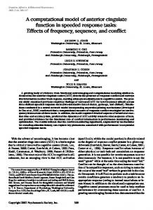
Figure 2: Typical fitness and diversity behaviour during evolution evolved individual in terms of its robustness. In this case, when referring to robustness of a phenotype we consider the ability of a phenotype to repair from damage at the phenotypic level. This was calculated by firstly growing a phenotype to maturity (figure 3a-d). Cells are randomly removed until only a small percentage of the original phenotype remains (figure 3e). The growth process is then reapplied until the previous number of cells have been reproduced (figure 3f-h). The robustness of a phenotype is then measured as the percentage of these cells which are spatially differentiated correctly according to the original template against which the individual was evolved. The phenotype is also robust to overgrowth, as seen in figure 3i, where cells are forced to overlap due to the limited size of the simulated space. Figure 4 shows the average response, for 10 evolutionary runs, to damage at both the genotypic and phenotypic levels of the most optimal individual in the population during a typical evolutionary process. Genotypic robustness is
100
80
Fitness (%)
60
40
20 Fitness of optimal individual in population Fitness after genotypic damage Fitness after phenotypic damage 0 0
50
100
150
200 250 300 Evolutionary Generations
350
400
450
500
100
Robustness (%)
80
Figure 3: Typical behaviour of optimal evolved phenotype in response to damage
60
40
20
a measure of the effects of a random single point gene mutation on the genotype by measuring the fitness of the resultant phenotype. Phenotypic robustness is calculated from the number of cells which match the target template after first culling cells randomly from a fully developed phenotype until only a given percentage remain, in this case 50%, and then reapplying the growth process until previous cell numbers have recovered. The robustness is a percentage measure of similarity to the original phenotype in terms of fitness. Robustness(%) = 100 ∗
F itnessInResponseT oDamage OriginalF itness (2)
Response to phenotypic damage gives the most clear results showing that a consistently high value of robustness is achieved whilst response to genetic mutations produces much noisier results which overall portray a much lower robustness capability. This suggests that phenotypic robustness, or another characteristic of which it is a by-product, is actively sought after by the evolutionary system. The hypothesis upon which this work is based is that the robustness characteristic of these phenotypes is a result of the formation of modules in the embryogeny mapping. In order to analyse this hypothesis the interaction between genes and specific features of the phenotype are analysed. This requires a set of distinct phenotypic features to be defined and for the French flag pattern the most obvious are of course the three differentiated sections of colour. If each gene is removed from the genome in turn, a dif-
Robustness to genotypic damage Robustness to phenotypic damage 0
0
50
100
150
200 250 300 Evolutionary Generations
350
400
450
500
Figure 4: Robustness of optimal phenotype during evolution ferent phenotype for each gene which has been deleted can be observed. Figure 5 shows the typical behaviour of the phenotype, for an optimal individual, to the removal of individual genes in this manner. For more than half of cases the resultant phenotype shows no change (figure 5a-b) whilst most others show alterations which can be specifically associated to these three distinct areas of differentiated colour in the original phenotype (figure 5c-h). For a more thorough assessment of this hypothesis it is necessary to define a measure of modularity. A gene is defined as belonging to a module if its effect on one of these phenotypic features is greater than upon any of the others [7]. Figure 6 shows the result of calculating the percentage of genes in a genome which can be considered modular according to the above definition. It is shown that, averaged over 10 evolutionary runs, the modularity of the most optimal genome increases over evolutionary time.
5 Discussion Traditionally, simulated evolution has been implemented around the concept of selection pressure. For this reason neutrality is often considered to be a detrimental feature of complex mappings since the predominant force behind
Figure 5: Phenotypes resulting from the removal of individual genes 50
6 Conclusion
45
Modular Genes (%)
40
35
30
25
20
15 0
isolate specific genes to identifiable features in the phenotype as seems to be the case in figure 6. This modularity in the mapping between genotype and phenotype may explain why phenotypes are robust to damage. The embryogeny mapping is a cyclic process since the phenotype is dependent upon the genotype and vice versa. This means that the canalizing behaviour of the mapping from genotype to phenotype can in effect be reversed. Disruptions in the mapping process caused by damage to the phenotype are localised by the modularisation and so only affect small parts of the genotype. This minimises the impact of damage and noise on the mapping process which might otherwise worsen with progressive growth. In essence, it is not the genotype or phenotype that exhibit canalized behaviours but the mapping process itself.
100
200 300 Evolutionary Generations
400
500
Figure 6: Measuring the average modularity of the most optimal genome during evolution evolution is disrupted. However, if selection pressure is replaced with random selection there is still a form of evolutionary drive. If we postulated that as fitness improves during evolution the number of individuals with greater or equal fitness is decreasing, then we can argue that random selection and search operators will become more damaging during evolution. Therefore an individual is more likely to survive if it is robust to damaging search operators, a process known as canalization. The results show that evolution causes canalization of the genotype such that small changes to the genotype tend to result in minimal or trait specific effects upon the phenotype, and that the phenotypes are themselves robust to damage. The question is how does this canalization occur and how does it relate to phenotype robustness? Pleiotropy describes the ability of a gene or group of genes to influence the behaviour of multiple phenotypic traits [1]. It can be argued that if levels of pleiotropy are high then search operators are more likely to affect multiple aspects of the phenotype. However if pleiotropy is maintained at low levels then search operators should be limited to affecting individual features of the phenotype. Results shown in figure 5 seem to strengthen this argument and a good way to maintain low levels of pleiotropy would be to
This paper has demonstrated how an evolutionary system utilising a complex mapping based on a model of embryogeny can produce some observable, measurable and repeatable effects on an evolutionary system. These effects consist of forming a modularisation in the complex mapping which results in specific traits in the phenotype being described by a specific group of genes in the genotype. It is this argument which is used as the basis for the following hypothesis. For a complex mapping, such as a model of embryogeny, useful traits are observed in the phenotype. For these traits to be effectively utilised in simulated evolution it must be possible to encapsulate these traits in the genotype. If the genotype is represented in such a way that genes which function together are grouped together then they become isolated in both the genetic and phenotypic representations. We call this a modularised mapping and how evolution attempts to untangle this mapping could have important implications. This work highlights a need to acknowledge the importance of distinguishing between genotypic and phenotypic representations and how their interaction influences simulated evolutionary systems. Such characteristics of an evolutionary system may be fundamentally useful in evolving more complex phenotypic structures. This approach has already been utilised for describing neural networks on a much lower level than most existing evolutionary neural network models [3, 15] and has the potential to overcome problems already highlighted for evolvable hardware [12, 8]. Future work is to produce comparative models with various forms of representations, including those which do not bias towards modular structures.
Acknowledgments This work is supported by the EPSRC through a Doctoral Training Account and the School of Computer Science at the University of Birmingham. The author wishes to express gratitude for the help and supervision provided by Dr John A. Bullinaria and for original inspiration and guidance provided by Dr Julian F. Miller.
Bibliography [1] L. Altenberg. Genome Growth and the Evolution of the Genotype-Phenotype Map. Lecture Notes in Computer Science, 899:205–259, 1995. [2] C. P. Bowers. Evolving Robust Solutions with a Computational Model of Embryogeny. In J. M. Rossiter and T.P. Martin, editors, Proceedings of the UK Workshop on Computational Intelligence: UKCI’2003, pages 181–188, Bristol, UK, 2003. University of Bristol. [3] C. P. Bowers and J. A. Bullinaria. Embryological Modelling of the Evolution of Neural Architecture. In A. Cangelosi, G. Bugmann, and R. Borisyuk, editors, Modelling Language, Cognition and Action, pages 375–384. World Scientific, 2005. [4] B. Alberts et al. Molecular Biology of the Cell. Garland, 3rd edition, 1994. [5] I. Harvey. Artificial Evolution for Real World Problems. In T. Gomi, editor, Evolutionary Robotics: From Intelligent Robots to Artificial Life: ER’97, pages 127–149. AAI Books, 1997. [6] S. Kumar and P. Bentley. Computational Embryogeny: Past, Present and Future . In Ghosh and Tsutsui, editors, Advances in Evolutionary Computing, Theory and Applications, pages 461–478. Springer, 2003. [7] C. Lam and F. G. Shin. Formation and Dynamics of Modules in a Dual-Tasking Multi-Layer FeedForward Neural Network. Phys. Rev. E, 58(3):3673– 3677, 1998. [8] H. Liu, J. F. Miller, and A. M. Tyrell. An Intrinsic Robust Transient Fault-Tolerant Developmental Model of Digital Systems. In J. F. Miller, editor, WORLDS Workshop, The Genetic and Evolutionary Computation Conference: GECCO’2004, Lecture Notes in Computer Science. Springer, 2004. [9] J. F. Miller and W. Banzhaf. Evolving the Program for a Cell: From French Flags to Boolean Circuits. In S. Kumar and P. Bentley, editors, On Growth, Form and Computers, pages 278–302. Academic Press, London, UK, 2003. [10] M. Nowostawski and R. Poli. Parallel Genetic Algorithm Taxonomy. In L. C. Jain, editor, Proceeding of the Third International Conference on Knowledge Based Intelligent Information Engineering Systems: KES’99, pages 88–92, Adalaide, 1999. IEEE. [11] C. Ortega, D. Mange, S. L. Smith, and A. M. Tyrrell. Embryonics: A Bio-Inspired Cellular Architecture with Fault-Tolerant Properties. Genetic Programming and Evolvable Machines, 1(3):187–215, 2000.
[12] V. K. Vassilev and J. F. Miller. Scalability Problems of Digital Circuit Evolution. In J. Lohn, A. Stoica, D. Keymeulen, and S. Colombano, editors, Proceedings of the 2nd NASA/DOD Workshop on Evolvable Hardware, pages 55–64, Los Alamitos, CA, 2000. IEEE Computer Society. [13] L. Verlet. Computer Experiments on Classical Fluids I. Thermodynamical Properties of Lennard-Jones Molecules. Phys. Rev., 159(98), 1967. [14] L. Wolpert. Positional Information and the Spatial Pattern of Cellular Differentiation. Journal of Theoretical Biology, 25(1):1–47, 1969. [15] X. Yao. Evolving Artificial Neural Networks. Proceedings of the IEEE, 87(9):1423–1447, 1999.