Mohamed W. Mehrez, George K. I. Mann, and Raymond G. Gosine. Intelligent ..... [9] J. Sanchez and R. Fierro, âSliding mode control for robot formations,â.
Formation Stabilization of Nonholonomic Robots Using Nonlinear Model Predictive Control Mohamed W. Mehrez, George K. I. Mann, and Raymond G. Gosine Intelligent Systems Lab, Faculty of Engineering and Applied Science Memorial University of Newfoundland St. John’s, NL, Canada A1C 5S7 Email: {m.mehrez.said, gmann, rgosine}@mun.ca Abstract—This paper compares two approaches of multirobots’ formation stabilization using nonlinear model predictive control (NMPC), namely, centralized and distributed predictive controls. Centralized NMPC has been highlighted in the literature to lead superior performance; however, it has been remarked with high computational power requirements which limit its application to practical formation stabilization problems. Nonetheless, in this paper, the use of a recently developed toolkit implementing fast NMPC algorithms rendered this problem tractable. The performance of the two control approaches are compared in a series of numerical simulations. The results demonstrated that the centralized controller has a better performance compared with its distributed counterpart. Furthermore, it showed realtime requirements satisfaction.
I.
I NTRODUCTION
Interest in formation control has been expanded in multirobot systems over the last two decades. This interest has grown primarily because some given tasks may be too complex to be achieved by a single working robot, or multiple robots can execute the same task faster with higher performance. Application areas of multiple robots include grid searching by coordinating robots, rescue, exploration, and surveillance using multiple unmanned air or ground vehicles [1]. In general, the formation control objective is to coordinate a group of robots to maintain a prescribed formation. The literature highlights different approaches of formation structures, where most of them can be categorized under virtual structure, behaviour based, and leader follower approaches. In the virtual structure approach, the robots’ formation is considered as a rigid body and the individual robots are treated as points on this body. The motion of the individual robots in the formation is then obtained from the overall motion of the formation. In behaviorbased control, several desired behaviors are assigned for each robot in the formation, including fromation keeping (stabilization), goal seeking, and obstacle avoidance. The fundamental approach of the leader follower structure is that a follower robot is assigned to follow the pose of another vehicle with an offset [2]. The solution to the virtual structure approach is presented in [3], where authors designed an iterative algorithm which fits the virtual structure to the positions of the individual robots in the formation, then displaces the virtual structure in a prescribed direction and then updates the robot positions. Solutions to the behaviour based approach include motor scheme control [4], null-space-based behaviour control [5], and social potential fields control [6]. The leader-follower
control approach is achieved using feedback linearization [7], backstepping control [8], sliding mode control [9], and model predictive control [10]. A nonholonomic motion (kinematic) model , e.g., unicycle, is a widely used model to describe vehicles kinematics in robots’ formations [11]. Nonlinear model predictive control (NMPC) has been seen to be a natural methodology to adopt in controlling systems governed by constrained dynamics [1]; In NMPC, a cost function is formulated to minimize the formation objective error and an optimal control input is obtained by solving a discrete nonlinear optimization problem over a pre-defined prediction horizon. Mobile robot control schemes including kinematic control and potential field control do not include the future state of the robots in formation to compute the current control actions. On the other hand, NMPC predicts the future state using the open loop robot model [12]. In formation control problems, centralized control laws can ideally yield superior performance and optimal decisions for the individual members and the whole formation. In this approach, a single controller oversees the decision process for the whole group. Moreover, it generates control actions which would lead to collision free trajectories in the workspace. Although this guarantees a complete solution, centralized algorithms have been highlighted in the literature to have high computational power demand [13]. On the other hand, in the decentralized control approaches, each formation member has its own controller and is completely autonomous in the decision process [14]. This can reduce the high computational power requirements; however, each robot in the formation cannot estimate precisely the behaviours of the other robots in the formation. In this paper, nonlinear model predictive control (NMPC) has been adopted to solve a multi-vehicle formation stabilization to a permissible equilibrium’s problem which is free from the leader-follower architecture, guided by [1]. Two formation stabilization NMPC schemes have been used, namely, centerlized scheme and decenterlized scheme; the control objective is set to stabilize the whole formation to a permissible equilibrium while considering work-space margins and obstacles. The use of a recently developed toolkit implementing fast NMPC algorithms (ACADO toolkit [15]) makes the realtime implementation of the centerlized controller feasible. The performance of the two controllers have been compared and contrasted in terms of performance measures and real-time requirements satisfaction.
The structure of the paper is as follows: Section II presents a brief description of differential drive robots and defines the formation stabilization problem for multi-robot systems. Section III shows the formulation of centralized and distributed NMPC highlighting the main differences between the two approaches. Simulation results are then presented and discussed in Section IV. Finally, conclusions and future work extensions are presented in Section V. II.
YI vi R2
In this section, the multi-robots formation problem is defined; a brief description of the individual robots kinematics, in the formation, is also presented. In this work, the formation objective is motivated by stabilizing a group of nonholonomic robots to a permissible equilibrium by the requirement that all formation’s members have equivalent tasks relative to the whole formation, i.e. the leader-follower architecture is not adopted here [1]. In addition, environment’s map constraints and obstacles are also considered. This formation objective can be seen in deploying a team of exploring robots in a constrained environment, or in a goal tracking task with a fixed goal position as presented in [14]. The formation objective is illustrated in Fig.1(a); as shown in the figure, a group of three robots has the task of manoeuvring, in a constrained work space with map margins and obstacles, from an initial configuration to a prescribed final configuration. The individual robots have to reach their destinations while avoiding collision with other team members and the work space obstacles. Each robot has been circumferenced with a virtual circle of radius (Rc ), which specifies the robot occupancy of the map that needs to be avoided by other robots. This paper considers the formation control of teams composed of differential drive nonholonomic robots Fig.1(b). The differential drive robot has two drive wheels and an extra balancing castor wheel. The linear speeds of the right (vr ) and the left (vl ) wheels define the control inputs: linear speed (v = (vr + vl )/2) and angular speed (ω = (vr + vl )/b), where b is the wheel base. The kinematic equations of any individual robot in the formation under the nonholonomic constraint of rolling without slipping are given as follows [11]: 0 0 ui 1 #
(1)
where the subscript i denotes the ith robot in the formation. The state and control signal vectors are denoted as xi = (xi , yi , θi )T ∈ R3 and ui = (vi , ωi )T ∈ R2 . As shown in Fig. 1(b), (xi , yi ) represents the Cartesian position of the robot in the world frame of reference (XI , YI ), and (θi ) represents the robot orientation measured from the positive (XI ) to the robot frame x-axis (xR ). Despite the simplicity of the model (1), it is sufficient to describe the nonholonomic constraints of the differential drive robots. As system (1) has the control-affine form (2) and the accessibility rank condition is globally satisfied [11], system given by (1) is controllable. " # " # x˙ i 0 cos(θi ) x˙ i = y˙ i = sin(θi ) vi + 0 ωi (2) 0 1 θ˙i
xR R3
obstacles
R3
yR
R1 R2 initial R1 configuration
(xi, yi) ωi
XI
XI
O
(a) Fig. 1.
θi
final configuration
O
P ROBLEM F ORMULATION
" # " x˙ i cos(θi ) vi cos(θi ) x˙ i = y˙ i = vi sin(θi ) = sin(θi ) ωi 0 θ˙i
map margins
YI
(b)
(a) Formation objective. (b) Differential drive robot.
In order to illustrate the formation control objective a reference robot is defined for each member in the formation. This reference robot has the reference state vector xir = (xir , yir , θir )T and a reference control vector uir = (vir , ωir )T , and subject to the same constraint as system (1). Thus, its kinematic motion model can be written as: " # " # x˙ ir cos(θir ) 0 vir cos(θir ) x˙ ir = y˙ ir = vir sin(θir ) = sin(θir ) 0 uir (3) ωir 0 1 θ˙ir
At this point, the main objective of the formation control can be stated as the simultaneous stabilization of each robot in the team with state xi to its corresponding reference robot with state xir , where the reference control vector uir has zero values for both linear and angular velocities reference. The formation controller should also consider the radius of each robot Rc as well as map margins and obstacles. In order to have a practical controller design, the controller should include robots’ inputs saturation margins. The following section presents two NMPC controller architectures (centralized and distributed) which solve the above mentioned problem. III.
M ODEL P REDICTIVE C ONTROL FOR F ORMATION S TABILIZATION
In this section, centralized and distributed NMPC for multirobots formation stabilization are presented. The cost function for each scheme, the prediction model, and the optimization problem constraints are also defined. A. Centralized NMPC In the centralized NMPC, a formation augmented model is formed, where its sub-models are the individual differential models for each robot in the formation. The augmented model is given as follows: x˙ a = fa (xa (t), ua (t))
(4)
where xa = [xT1 , xT2 , ..., xTk ]T ∈ R3k is the augmented state vector of the k robots involved in the formation; ua = [uT1 , uT2 , ..., uTk ]T ∈ R2k is the augmented control actions vector for the whole robots; and fa : R3k × R2k → R3k is the nonlinear mapping formed by the individual robots’ models (1). The control objective is to compute an admissible control input u∗a (t) to drive system (4) to move toward the
formation equilibrium point defined by (xae (t) = xar (t) − xa (t) = 0 and uae (t) = uar (t) − ua (t) = 0 ), where xar = [xT1r , xT2r , ..., xTkr ]T ∈ R3k is the augmented vector of all robots references and uar = [uT1r , uT2r , ..., uTkr ]T ∈ R2k is the augmented vector of the reference control values which is zero in the formation stabilization case. The objective of the control algorithm is to minimize a weighted cost function over a prediction horizon T given by [1]: J(t, xae (t), uae (t)) =F (xae (t + T ))+ Z t+T ℓ(τ, xae (τ ), uae (τ ))dτ
(5)
t
where ℓ(τ, xae (τ ), uae (τ )) is the running cost function which is integrated over the the prediction horizon T and given by: ℓ(τ, xae (τ ), uae (τ )) =
k X
(xTei (τ )Qi xei (τ )+uTei (τ )Ri uei (τ ))
i=1
(6) F (xae (t + T )) is the terminal state penalty, evaluated at the end point of the optimization horizon, and given by: k
1X T ℓ(τ, xae (τ ), uae (τ )) = x (τ )Pi xei (τ ) 2 i=1 ei
(7)
where Qi , Ri , and Pi are positive definite symmetric weight matrices defined for each robot in the formation, and xei and uei are the state vector error and the control vector error for each robot, respectively. In order to avoid collision between robots and avoid obstacles in the environment, at time t, the online-open-loop optimization problem of the centralized NMPC controller can be outlined as the following: min J(t, xae (t), uae (t)) ua
subject to: x˙ a = fa (xa (t), ua (t)) ua (τ ) ∈ U, (τ ∈ [t, t + T ]) xa (τ ) ∈ X, (τ ∈ [t, t + T ])
(8)
where the set X ∈ R3k and the set U ∈ R2k specify the admissible regions of both states and control which are defined by the following set of constraints. First, the box constraints for robots inputs’ saturation limits as well as the map margins are given by:
B. Distributed NMPC Although rare work can be found, in the literature, where the centralized NMPC has been applied to non-holonomic robots’ formations, distributed control has been adopted in many studies implementing formation control. For example, in [16], a distributed NMPC has been applied to a nonholonomic robots’ formation, where the control objective is to maintain a specified formation pattern while tracking a predefined formation reference. A distributed NMPC applied to a formation of holonomic robots has been also presented in [14], where authors adopted a distributed NMPC to converge a group of mobile robots toward a desired target position. In the centralized NMPC, a single controller is used to process all the information of robots current measurements and their future evolution; however, under the distributed control pattern, each robot in the formation runs an NMPC controller individually while the whole formation information are shared between robots via a communication protocol [14]. In the distributed case, each robot in the team runs an NMPC controller with the same objective (5) subjected to the constraints equations (8) to (11); however, the future prediction of the robot own states and other team members’ states are not obtained as in the centralized case. Instead of the augmented motion model (4), each robot in the formation adopt model (1) for the future prediction of its own state vector; furthermore, it predicts the future states of the other robots based on their last known velocities, which are assumed to be constant over the prediction horizon [14]. Under the two formation controllers, the constrained online-optimization of the cost function (5), which considers the equilibrium state of the formation as well as the locations of obstacles, eliminates the need of the path planner layer which usually needs another control layer. It has to be mentioned here that the constraints (10) and (11) can also be embedded in the objective function (5) as a penalized potential field functions [17]. IV.
S IMULATION R ESULTS
Second, to achieve inter-robots collision avoidance, the following set of constraints is imposed on the optimization problem (7): ∀i, j : (xi − xj )2 + (yi − yj )2 ≥ 4Rc2 (10) i6=j
Due to advancements in computing machines and developments of efficient numerical algorithms, a considerable number of dynamic optimization and NMPC implementation packages has been developed [18], [19]. In this paper, the MATLAB interface of a software environment for automatic control and dynamic optimization (ACADO-Toolkit [15]) has been utilized to apply the two controllers designs presented in the previous section. The adopted toolkit is a recently developed package, which implements real-time NMPC routines, and has been proven to be open source, user friendly, extensible, selfcontained, and computationally versatile, when compared with the previously developed optimization packages [15].
Finally, to avoid obstacles in the environments (here assumed to have elliptical shapes), the following constraints are also considered: (xi − xobs )2 (yi − yobs )2 ∀i : + ≥1 (11) a2 b2 where a and b are ellipse parameters, and xobs and yobs are the coordinates of the ellipse center.
Under the two controllers design, the control objective is to coordinate a formation of three robots (k = 3) to manoeuvre in a given map from an initial configuration to a final one; in addition, while manoeuvring, robots must avoid collision with each other and any obstacle in the map. The map margins are specified by the pairs (xmin , xmax ) and (ymin , ymax ), and each member in the formation has input saturation limits defined by the pairs (vmin , vmax ) and (ωmin , ωmax ).
∀i :
vmin ≤ vi ≤ vmax ωmin ≤ ωi ≤ ωmax xmin ≤ xi ≤ xmax ymin ≤ yi ≤ ymax
(9)
Distributed NMPC
The three robots start from the initial configuration specified by x1 = (1(m), 1(m), 0(rad))T , x2 = (1, 2, 0)T , and x3 = (1, 3, 0)T , while the final formation configuration is defined as x1r = (6.5, 4, 0)T , x2r = (6, 6, 0)T , and x3r = (6, 2, 0)T . In this case, the controller saturation limits are adopted from [20], and the box constrains (9) have been chosen as: ∀i : −0.25 ≤ vi ≤ 0.6(m/s) − 0.7 ≤ ωi ≤ 0.7(rad/s) 0 ≤ xi ≤ 8(m) 0 ≤ yi ≤ 8(m)
8 robot1 robot2 robot3
7
6
y−position (m)
5
4
3
2
For the inter-robots collision avoidance, the robot radius Rc in (10) is chosen as Rc = 0.25(m). In addition, two elliptical obstacles have been placed in the map to assess the performance of the formation stabilization controllers. The first one is placed at (xobs1 = 3(m), yobs1 = 1.5(m)), while the second one is placed at (xobs2 = 3.5, yobs2 = 6.5); the parameters a and b shown in constraint (11) are chose as (a = 1.5(m), b = 0.5(m)) for the two obstacles. In order to assess the performance of the two controllers under the same given conditions, the weight matrices appear in (6) and (7) are chosen as: " # � � 0.5 0 0 20 0 Qi = Pi = 0 2 0 , and Ri = . 0 60 0 0 0.5 Under the two controllers, the prediction horizon parameters are defined as: the time step ∆T = 0.3 (seconds), and the total number of horizon steps N = 30 (steps) leading to a prediction horizon length of T = 9 (seconds). The total simulation time is chosen as 60 (seconds). The NMPC controllers (centralized and distributed) were implemented by two different methods of ACADO’s MATLAB interface. The Centralized controller is implemented completely in ACADO’s (simulation environment) MATLAB interface, where the optimal control problem is defined, as well as the system model (4); when the code is compiled and run, ACADO performs both the optimal control computation, and system states integration. The optimal control problem is solved based on the single-shooting Sequential Quadratic Programming (SQP) method, and states integration is achieved
1
0
Fig. 3.
0
1
2
3
4 x−position (m)
5
6
7
8
Formation robots’ performed trajectories (distributed NMPC)
by the Runge-Kutta integrator (of order 2/3). The KKT tolerance (Karush-Kuhn-Tucker: first order (necessary) optimality condition), which is used as a convergence criterion of the SQP algorithm, was set to 10−6 (default value in ACADO). In addition, the maximum number of iterations was also kept at its default value (1000). Readers can find more details about ACADO for MATLAB in [21]. The distributed control was implemented using the (stand-alone controller) feature of ACADO, where only the optimal control problem is defined. The stand-alone controller is then used by all robots in the formation, where robots last known speeds and states are shared and used for the calculation of the optimal control actions for each robot. Same controller options set for the centralized controller were adopted for the distributed one. All simulations were performed on a quad-core machine of 2.9 GHz processor and 8 GB of memory. Fig. 2 to Fig. 7 summarize the simulation results under the two controllers. Fig. 2 and Fig. 3 (best viewed in colors) show the three robots executed trajectories under the two controllers, respectively. The figures show the map margins as well as the elliptical obstacles’ positions and dimensions. Robots trajectories traces as well as 6 snap shots of their poses along the executed
Centralized NMPC
8 x−position (m)
8 robot1 robot2 robot3
7
6 4
robot1 robot2 robot3
2
6 0 8
0
10
20
30
40
50
60
0
10
20
30
40
50
60
0
10
20
30 time (sec)
40
50
60
y−position (m)
y−position (m)
5
4
3
6 4 2 0
1.5 theta (rad)
2
1
0
Fig. 2.
0
1
2
3
4 x−position (m)
5
6
7
0 −0.5
8
Formation robots’ performed trajectories (centralized NMPC)
1 0.5
Fig. 4.
Robots’ state vector xi components (centralized NMPC)
0.6
6
0.5
4
robot1 robot2 robot3
2 0 8
robot1 robot2 robot3
0.4
0
10
20
30
40
v (m/sec)
x−position (m)
8
50
0.3 0.2 0.1
60
y−position (m)
0
6 −0.1
4
1
0
5
10
15
20
25
30
0
5
10
15 time (sec)
20
25
30
2 0.5
0
10
20
30
40
50
60
ω (rad/sec)
0
theta (rad)
2
0
1 −0.5
0 −1
−1
0
10
20
30 time (sec)
40
50
60
Fig. 7. Fig. 5.
Robots’ controls vector ui components (distributed NMPC)
Robots’ state vector xi components (distributed NMPC)
trajectories are also shown. Robot’s snap shots along the trajectories are illustrated by arrows which represent the position and the orientation of the corresponding robot at the time the snap shot is taken. As can be noticed from the two figures, the formation controllers drove successfully the whole formation from the initial configuration to the final one; however, the executed trajectories and the final pose error per each robot are not the same under the two controllers. Performed trajectories appear to be smoother under the centralized controller than that for the distributed controller. In addition, by observing the third snapshot of each robot, the first robot in the formation appears to be the last robot leaving the congestion formed by the two ellipses under the centralized controller. On the other, under the distributed controller, the third robot is the one that leaves the congestion at last. Fig. 4 and Fig. 5 show the state vector xi components of each robot in the formation under the two applied controllers. The centralized controller shows again a smoother transition of the robots states, along the simulation time, than that of the distributed controller. Furthermore, the states show faster convergence to their reference values under the centralized controller. Fig. 6 and Fig. 7 show the control actions (vi , ωi ) applied to each robot; the control actions are plotted only 0.7 robot1 robot2 robot3
0.6
v (m/sec)
0.5 0.4 0.3 0.2 0.1 0
0
5
10
15
20
25
30
0.5 0.4
for the first 30 (seconds) of the simulations in order to magnify the contrast between the control actions under the two controllers. As can be inferred from the two figures, although the control actions didn’t go beyond their saturation limits (9), the centralized control shows smoother control actions than the control actions of the distributed control. The nonsmooth control actions generated by the distributed NMPC is because of the fact that, when a robot is calculating its own control actions, the last know velocities of the other robots in the formation are assumed to be constant over the prediction horizon. Table I summarizes the performance parameters P of the formation stabilization results under the two controllers. The performance parameters include the steady state error in the pose vector for each robot (xei (m) = xir − xi , yei (m) = yir − yi , and θei (rad) = θir − θi ),Pand the integral of norm α 2 squared actual control inputs γi = j=1 (kui,j k ∆T ), where α is the number of the controller update steps and ∆T is the used time step (seconds). γi is used as a metric to evaluate the control energy expenditure by each robot in the formation [11]. As can be seen in Table I, the centralized controller shows a better overall performance in terms of the steady state error; furthermore, the centralized controller shows also a more conservative energy expenditure for the all robots than that for the distributed controller. The average computational capacity requirements, per time step, under each controller have been observed to be 0.04 (seconds) for the distributed controller and to be 0.0625 (seconds) for the centralized one. Indeed, as the number of the formation members increases, the computational capacity demand of the centralized controller will significantly increase when compared with the distributed controller. As per the above analysis, the centralized NMPC formation control over performed the distributed one for nonholonomic
ω (rad/sec)
0.3
TABLE I.
0.2
0 −0.1 −0.2
Fig. 6.
F ORMATION S TABILIZATION P ERFORMANCE PARAMETERS
0.1
0
5
10
15 time (sec)
20
25
30
Robots’ controls vector ui components (centralized NMPC)
P xe ye θe γ
Centralized NMPC R1 R2 R3 0.031 0.056 0.013 −0.148 −0.138 −0.031 0.022 −0.01 0.029 7.260 7.236 5.29
Distributed NMPC R1 R2 R3 −0.18 −0.165 −0.228 −0.103 −0.114 −0.106 0.403 0.376 0.463 8.557 8.637 7.247
formations stabilization to a permissible equilibrium. The reason behind this lies in the fact that the centralized controller overseas the overall performance of the formation, while the distributed controller does the prediction based on the last known robots’ velocities. Although the centralized controller showed a superior performance and real-time requirements satisfaction, its scalability is limited to a certain number of formation members. In addition, while the simulation results always show convergence of the formation robots to their references, the stability of the adopted method here needs to be investigated. V.
C ONCLUSION
In this work, formation stabilization is achieved by means of two nonlinear model predictive controllers, namely, centralized NMPC and distributed NMPC. In order to prepare the centralized controller for real-time applications, a recently developed toolkit, which implements fast NMPC routines, has been adopted to solve the computational capacity requirement of the centralized controller. The two controllers have been applied to a formation stabilization problem, which is free from the leader-follower architecture. In a numerical simulations context of formation stabilization, in a map with obstacles, a superior performance of the centralized controller has been observed, while the real-time requirements are satisfied. The future work of this research include the stability assessment of the centralized controller as well as the realtime experimental validation of the formation stabilization. ACKNOWLEDGMENT This work is supported by Natural Sciences and Engineering Research Council of Canada (NESRC), the Research and Development Corporation (RDC), C-CORE J.I. Clark Chair, and Memorial University of Newfoundland. R EFERENCES [1] W. Dunbar and R. Murray, “Model predictive control of coordinated multi-vehicle formations,” in Decision and Control, 2002, Proceedings of the 41st IEEE Conference on, vol. 4, pp. 4631–4636 vol.4, 2002. [2] M. Saffarian and F. Fahimi, “Non-iterative nonlinear model predictive approach applied to the control of helicopters group formation,” Robotics and Autonomous Systems, vol. 57, no. 67, pp. 749 – 757, 2009. [3] M. Lewis and K.-H. Tan, “High precision formation control of mobile robots using virtual structures,” Autonomous Robots, vol. 4, no. 4, pp. 387–403, 1997. [4] T. Balch and R. Arkin, “Behavior-based formation control for multirobot teams,” Robotics and Automation, IEEE Transactions on, vol. 14, no. 6, pp. 926–939, 1998. [5] G. Antonelli, F. Arrichiello, and S. Chiaverini, “Flocking for multirobot systems via the null-space-based behavioral control,” in Intelligent Robots and Systems, 2008. IROS 2008. IEEE/RSJ International Conference on, pp. 1409–1414, 2008. [6] T. Balch and M. Hybinette, “Social potentials for scalable multi-robot formations,” in Robotics and Automation, 2000. Proceedings. ICRA ’00. IEEE International Conference on, vol. 1, pp. 73–80 vol.1, 2000. [7] G. Mariottini, F. Morbidi, D. Prattichizzo, G. Pappas, and K. Daniilidis, “Leader-follower formations: Uncalibrated vision-based localization and control,” in Robotics and Automation, 2007 IEEE International Conference on, pp. 2403–2408, 2007. [8] X. Li, J. Xiao, and Z. Cai, “Backstepping based multiple mobile robots formation control,” in Intelligent Robots and Systems, 2005. (IROS 2005). 2005 IEEE/RSJ International Conference on, pp. 887–892, 2005.
[9] J. Sanchez and R. Fierro, “Sliding mode control for robot formations,” in Intelligent Control. 2003 IEEE International Symposium on, pp. 438– 443, 2003. [10] D. Gu and H. Hu, “A model predictive controller for robots to follow a virtual leader,” Robotica, vol. 27, pp. 905–913, 10 2009. [11] F. Xie and R. Fierro, “First-state contractive model predictive control of nonholonomic mobile robots,” in American Control Conference, 2008, pp. 3494–3499, 2008. [12] H. Lim, Y. Kang, J. Kim, and C. Kim, “Formation control of leader following unmanned ground vehicles using nonlinear model predictive control,” in Advanced Intelligent Mechatronics, 2009. AIM 2009. IEEE/ASME International Conference on, pp. 945–950, 2009. [13] K. Kanjanawanishkul, Coordinated Path Following Control and Formation Control of Mobile Robots. PhD thesis, Universitt Tbingen, Wilhelmstr. 32, 72074 Tbingen, 2010. [14] T. P. Nascimento, A. P. Moreira, and A. G. S. Conceio, “Multi-robot nonlinear model predictive formation control: Moving target and target absence,” Robotics and Autonomous Systems, vol. 61, no. 12, pp. 1502 – 1515, 2013. [15] B. Houska, H. Ferreau, and M. Diehl, “ACADO Toolkit – An Open Source Framework for Automatic Control and Dynamic Optimization,” Optimal Control Applications and Methods, vol. 32, no. 3, pp. 298–312, 2011. [16] S.-M. Lee and H. Myung, “Cooperative particle swarm optimizationbased predictive controller for multi-robot formation,” in Intelligent Autonomous Systems 12 (S. Lee, H. Cho, K.-J. Yoon, and J. Lee, eds.), vol. 194 of Advances in Intelligent Systems and Computing, pp. 533– 541, Springer Berlin Heidelberg, 2013. [17] T. Teatro and J. Eklund, “Nonlinear model predictive control for omnidirectional robot motion planning and tracking,” in Electrical and Computer Engineering (CCECE), 2013 26th Annual IEEE Canadian Conference on, pp. 1–4, 2013. [18] D. B. Leineweber, I. Bauer, H. G. Bock, and J. P. Schlder, “An efficient multiple shooting based reduced sqp strategy for large-scale dynamic process optimization. part 1: theoretical aspects,” Computers and Chemical Engineering, vol. 27, no. 2, pp. 157 – 166, 2003. [19] L. Simon, Z. Nagy, and K. Hungerbuehler, “Swelling constrained control of an industrial batch reactor using a dedicated nmpc environment: Optcon,” in Nonlinear Model Predictive Control (L. Magni, D. Raimondo, and F. Allgwer, eds.), vol. 384 of Lecture Notes in Control and Information Sciences, pp. 531–539, Springer Berlin Heidelberg, 2009. [20] M. Mehrez, G. Mann, and R. Gosine, “Stabilizing nmpc of wheeled mobile robots using open-source real-time software,” in Advanced Robotics (ICAR), 2013 16th International Conference on, pp. 1–6, Nov 2013. [21] D. Ariens, B. Houska, and H. Ferreau, “Acado for matlab user’s manual.” http://www.acadotoolkit.org, 2010–2011.