Random projection for non-Gaussian mixture models
Győző Gidófalvi Department of Computer Science and Engineering University of California, San Diego La Jolla, CA 92037
[email protected]
Abstract Recently, random projection, a key dimensionality reduction technique, was successfully incorporated into the learning of mixture of Gaussians with the EM algorithm. In this work we examine the possibility of incorporating random projection to into the learning of other mixture models. More specifically, we use random projection in conjunction with EM for mixture of Gaussians to learn a high dimensional probabilistic graphical model. In our experiments we find that while the model learned by the method that incorporates random projection does not learn the same accurate model as the one which does not, the models learned are qualitatively and structurally very similar.
1
Introduction
One commonly used method for modeling data is the mixture of Gaussians. It assumes that the n-dimensional data was generated by k n-dimensional Gaussians. The mixture and parameters of these k-Gaussians can be efficiently learned using the popular Expectation Maximization (EM) algorithm. The popularity of mixture of Gaussians is due to the fact that a large amount of natural data is Gaussian-like, and due to the simplicity and efficiency of the learning algorithm available for this model. However learning models for high dimensional data still poses challenges. First, to learn a model that generalizes well on novel test patterns one must have access to an exponential number data points. This is often referred to as the curse of dimensionality. Second, the running time complexity of most learning algorithms is a polynomial function of the dimensionality of the data. Recently in [2], Dasgupta proposed a new and simple scheme to solve these challenges. As Dasgupta suggested, a high dimensional mixture of Gaussians may be learned by first projecting the data down to a subspace of lower dimension where learning is less challenging and more efficient. This proposed method was motivated by the two recent theoretical results about random projection. Namely that after projecting data generated by a mixture k Gaussians down to O(log k)
dimensions the projected data approximately has the same level of separation between the k clusters as the original data had in high dimension. Furthermore data obtained after random projections appears to be more spherical. The advantages of this scheme achieved by random projections are obvious. Its effectiveness were demonstrated in a serious of tests in [2]. Based on the results by Diaconis et. al. that a variety of non-Gaussian highdimensional data appears to be more Gaussian in lower dimension, one could imagine that the simple scheme proposed by Dasgupta could be applied to learn different mixture models. This is the focus of this paper. In particular we try to apply this simple scheme to the mixture of trees model by Meilǎ [4]. We empirically evaluate the mixture of trees model learned using this simple scheme and compare it to a mixture of trees model that is learned in the high dimensional input space. In the following sections we briefly review the simple scheme incorporating random projection for learning a mixture of k-Gaussians, tree distributions and mixture of trees. We then apply this simple scheme to learn a mixture of trees model. This is followed by the description of our experiments and its results. Finally, we end our paper with future work and conclusions sections.
2
Random projection
A simple scheme that incorporates the advantages of random projection and the EM algorithm was presented in [2]. The following is a simple high-level outline taken from [2]: •
Project the date into a randomly chosen d-dimensional subspace.
•
Run EM to convergence on the low-dimensional data.
•
Take the fractional labels from EM’s final soft-clustering of the lowdimensional data, and apply these same labels to the original high-dimensional data. This yields estimates of the high-dimensional means, covariances, and mixing weights.
•
Run EM for one step in the high dimension.
The extensive experiments carried out by Dasgupta showed that this simple method matched the performance of the traditional method of learning a mixture of Gaussians in high dimension. There are a number of advantages to this method. First, it reduces the dimensionality of the training data, thereby making the learning task possible even if the number of example in high dimension is insufficient. Second, since in the randomly chosen subspace clusters are more spherical, the shortcomings of EM due to random initialization is somewhat reduced [2]. Finally, learning the mixture weights in lower dimension is more efficient.
3
Mixtures of trees
Mixture of trees by Meilǎ et. al [4] is a probabilistic graphical model for performing density estimation, prediction or classification in maximum likelihood and Bayesian framework. These trees are somewhat more restrictive than general Bayesian networks, however both their parameters and structures can be learned more efficiently. Before we make further reference to mixture of trees let us review tree models.
Tree distributions are a restricted version of probabilistic graphical models for which both the structure of the model and its parameters can be learned in an efficient way as it was shown in [4]. The algorithm that finds these two components such that the likelihood of a set of observations is maximized is known as the Chow-Liu algorithm. To give an overview of the Chow-Liu algorithms, let us first introduce the tree model for representing the distribution of over n discrete random variables similar to how it was introduced in [4]. For a set of n discrete random variables V , and observations of those random variables D={x1, x2, …, xN}, where xi∈{0,1}n and i=1...N, define a tree distribution as follows. Represent every random variable u as a node in the tree. For every u,v∈V and (u,v)∈E, let Tuv denote the joint probability distribution on u and v. Given that we denote the marginal of Tuv with respect to u for any v ≠ u as Tu, we can assign a distribution T to the graph (V,E) as follows:
T ( x) =
∏ ∏
( u ,v )∈E
Tuv ( xu , xv )
T ( xv )deg v−1 v∈V v
,
(1)
where deg v is the degree of vertex v. The learning problem for tree distributions can be formulated as follows. Find T*, such that: N
T * = arg max ∑ log T ( xi ) . T
(2)
i=1
The Chow-Liu algorithm solves the learning problem in quadratic time in terms of n in three steps. As the first step it computes the pairwise marginals Puv for all u and v. This is an empirical distribution over V. As the second step, from these marginals it computes the mutual information between every pair or variables under the distribution of P. Finally, as the third step it computes the maximum-weight spanning tree of (V,E) using the mutual information computed in the previous step as edge weights. The following figure formalizes these steps. Input: Distribution P over domain V 1. 2. 3. 4.
Given a distribution P over V compute pairwise marginals Puv ∀u,v∈V Compute mutual information Iuv ∀u,v∈V Compute the maximum spanning tree ET of {Iuv} Set Tuv ≡ Puv for (u,v)∈ ET
Output: T Figure 1: Chow-Liu algorithm for learning a tree distribution T over domain V. Meilǎ et. al present a simple iterative EM-type algorithm in [4], which in the maximization step invokes the Chow-Liu algorithm to determine the structure and parameters of the individual mixture components and in the expectation step calculates the likelihood of the data as a function of the new model parameters, given the current model parameters.
4
Random projection for mixture of trees
Diaconis et. al. showed that a variety of non-Gaussian high-dimensional data appears to be more Gaussian in lower dimension. Based on these results as Dasgupta suggested in [2], one can imagine that the simple scheme for learning mixture of Gaussians via random projection may generalize to any mixture model, including mixture of trees. This would entail the following simple steps: 1. Randomly project high-dimensional data 2.
Learn a mixture of Gaussians in low dimension
3.
Use low-dimensional soft-clustering to learn high-dimensional component distribution
One can think of step 2 as learning a coarse clustering of the data. Similarly one can think one can think of step 3 as a refinement of the model which is achieved by learning the parameters and structure of the trees in high dimensions. This refinement could allow the model to capture information about the data that was not preserved during the random projection. The clear advantages of this method over a the method that tries to learn a mixture of tree model in high dimension is that learning the coarse structure of data in low dimension is more efficient and more tractable then in high dimension. At the same time, we hypothesize that the final high-dimensional model learned with this method has similar representation of the data to the representation of a model that is learned in high dimension only.
5
Experiments
We compare the performance of the two methods (mixture of trees using random projection (MTRP) vs. mixture of trees learned in high dimension (MTHD)) on the bit-mapped digit recognition / classification task. We would like to emphasize here that the point of this experiment is not to show the absolute performance of these two methods, but rather to try to measure relative performance between them and to discover similarities and differences between the models learned by the two methods. 5.1
Dataset
We compare the performance of the two methods on the bit-mapped digit recognition task. We use the NIST hand-written digit dataset. This dataset consists of 60,000, 28 x 28 pixel grayscale images of digits. We randomly select 700 images of each digit class as our training set and also randomly select 70 images per digit class as out test set. To further reduce our computation task we resized the selected images to 16 x 16 pixels and converted to black and binary images. This later change was necessary because we developed software for the mixture of trees only for discrete random variables. These images are represented as vectors in the {0,1}256 space and heron are referred to interchangeably as data points.
5.2
Experimental setup
To perform the recognition / classification task on our dataset we construct a Bayesian classifier by first learning a generative model (i.e.: mixture of trees) for each digit class and assign a novel test data point to the digit class whose mixture model assigns the highest likelihood to that test data point. For the MTRP method, based on the results by Dasgupta [2], we have chosen d to be 40, that is the randomly chosen subspace For both methods we have only experimented with a fixed value of k=5. This means that in both cases a particular digit class is modeled by a mixture of 5-trees. Here the different mixture components could possibly represent different styles of a particular digit class. 5.3
Results
Based on 10 randomly initialized test, we find that the classification accuracy of MTHD is 76.87% with a standard deviation of 1,153, while the classification accuracy of MTRP is 66.7% with a standard deviation of 2.049. These results suggest that the models learned by the two methods is significantly different. However a closer look to the confusions matrices reveals substantial similarities. For each of the methods figure 2 shows the average of the confusion matrices produced by the 10 test runs. The upper half of the figure shown the confusion matrices for the MTHD, while the lower half shows the averaged confusion matrix for the In the confusion matrices rows represent the actual classes while columns represent predicted classes. So the (i,j)th entry of a confusion matrix records the number of times class j was predicted when class i was the true class. In the confusion matrices the bold, diagonal entries show the number of correctly classified data points for each class. Besides the obvious that these entries for the MTRP are generally lower than the corresponding entries for the MTHD, one can see that the same classes are confused more with other classes for both of the two different models. For example digit class "1" is mostly classified correctly by both models, while digit class "8" is classified the least accurately. Furthermore it is also important to pay attention to the classes labels that a particular class model is confused with. The representative entries of this phenomenon are italicized in both of the matrices. From the results id seems that the models learned by the two different methods confuse corresponding digit classes with the same digit classes. For example for both models is true that digit class "4" is mostly confused with digit class "9". While our results suggest that the model learned by MTRP does not have the same accuracy as the one learned by MTHD, a closer investigation by looking at the averaged confusion matrices suggests that the two models learned are perhaps qualitatively similar. This partially agrees with out initial hypothesis that the two models learned will have similar representation of the data. Perhaps, to achieve a closer similarity in representations of the models, since data in higher dimensions are less likely to be Gaussian, it would make sense to perform a few EM steps of a model that does not make the Gaussian assumption (i.e.: mixture of trees). This approach would allow more time to refinement of the model in high dimensions while still being more efficient and tractable.
Mixture of trees in high dimension Confusion matrix
Predicted class "0" "1" "2" "3" "4" "5" "6" "7" "8" "9"
"0" 56.70 0.00 1.40 2.40 0.40 4.40 2.20 0.30 2.00 0.20 "1" 0.00 67.10 0.10 0.60 0.70 0.10 0.10 0.30 0.90 0.10 "2" 0.30 1.70 55.10 3.50 1.40 1.40 1.30 2.20 2.70 0.40 "3" 1.30 1.20 3.00 47.30 0.80 7.00 1.00 1.30 4.80 2.30 "4" 0.20 0.30 1.10 0.30 50.30 0.90 1.00 2.50 0.60 12.80 "5" 0.60 0.00 2.20 5.70 1.30 49.70 1.40 1.40 5.60 2.10 "6" 1.80 0.50 2.40 0.90 1.40 3.30 57.30 0.30 1.70 0.40 "7" 0.20 0.10 0.10 0.50 4.60 0.90 0.40 53.60 0.40 9.20 "8" 1.60 0.50 5.60 4.60 1.10 3.40 3.10 1.30 46.90 1.90 "9" 0.00 0.20 0.30 1.70 6.20 0.70 0.30 5.80 0.70 54.10
Actual class
Mixture of trees with random projection Confusion matrix
Actual class
Predicted class "0" "1" "2" "3" "4" "5" "6" "7" "8" "9"
"0" 53.20 0.00 2.10 1.70 1.10 4.10 2.70 1.20 2.80 1.10 "1" 0.00 66.70 0.30 0.10 0.50 0.40 0.20 0.50 1.20 0.10 "2" 1.70 2.40 42.70 6.70 2.50 3.30 3.30 2.00 3.90 1.50 "3" 1.90 1.90 3.50 40.10 1.40 9.10 1.40 1.80 6.40 2.50 "4" 0.40 1.00 2.40 0.80 40.30 2.20 2.90 2.90 1.80 15.30 "5" 2.30 1.10 2.70 6.40 3.20 40.60 3.10 2.40 5.50 2.70 "6" 2.50 0.50 2.30 1.70 4.10 3.80 52.60 0.30 1.30 0.90 "7" 0.70 0.20 0.80 0.60 5.40 2.80 0.20 49.00 1.10 9.20 "8" 3.10 1.30 5.90 6.40 3.80 5.30 4.10 2.30 34.30 3.50 "9" 0.10 0.60 0.60 1.10 7.70 2.80 0.80 5.70 1.60 49.00
Figure 2: Averaged confusion matrices for the tow methods. Top half shows the result obtained by MTHD while the bottom half shows the result obtained by MTRP. In both cases rows represent actual classes while columns represent predicted classes.
6
F u t u r e wor k
Our initial results suggest that a slightly modified method that would allow for a few EM steps in high dimension (more refinement) would match result in a more similar representation of the data for the two models. Other qualitative evaluation methods such as randomly sampling the two models for each digit class or perhaps randomly sampling individual mixture components would allow further in depth structural analysis.
7
Conclusions
Recently, random projection, a key dimensionality reduction technique, was successfully incorporated into the learning of mixture of Gaussians with the EM algorithm. In this work we examine the possibility of incorporating random projection to into the learning of other mixture models. More specifically, we use random projection in conjunction with EM for mixture of Gaussians to learn a high dimensional probabilistic graphical model. In our experiments we find that while the model learned by the method that incorporates random projection does not learn the
same accurate model as the one which does not, the models learned are qualitatively and structurally very similar. Acknowledgments I would like to thank Sanjoy Dasgupta for his thoughtful comments and for the code he provided for randomized projection. References [1] Chow, C. K., & Liu, C. N. (1978) Approximating Discrete probability distributions with dependency trees. IEEE Transactions on Information Theory IT14, 3, 462-467. [2] Dasgupta, S. (2000) Experiments with random projection. Uncertainty in Artificial Intelligence (UAI). [3] Diaconis, P. & Freedman, D. (1984) Asymptotics of graphical projection pursuit. Annals of Statistics, 12:793-815. [4] Meilǎ, M. & Jordan, M. (2000) Learning with mixture of trees. Journal of machine Learning Research.