Dec 8, 2004 - Finite Element Model Version 44.XX. Rick Luettich. University of North Carolina at Chapel Hill. Institute of Marine Sciences. 3431 Arendell St.
Formulation and Numerical Implementation of the 2D/3D ADCIRC Finite Element Model Version 44.XX
Rick Luettich University of North Carolina at Chapel Hill Institute of Marine Sciences 3431 Arendell St. Morehead City, NC 28557 Joannes Westerink Department of Civil Engineering and Geological Sciences University of Notre Dame Notre Dame, IN 46556
12/08/2004
1
TABLE OF CONTENTS
1.0 CONTINUITY EQUATION______________________________________________ 3 2.0 2D MOMENTUM EQUATIONS _________________________________________ 15 3.0 3D MOMENTUM EQUATIONS _________________________________________ 30 4.0 VERTICAL VELOCITY _______________________________________________ 50 5.0 SPERHICAL COORDINATE FORMULATION ___________________________ 53 6.0 LATERAL BOUNDARY CONDITIONS __________________________________ 57 7.0 BAROCLINIC PRESSURE GRADIENT CALCULATION NOTES
__________ 67
8.0 APPENDIX - BASIC CALCULATIONS ON LINEAR TRIANGLES
_________ 68
9.0 REFERENCES________________________________________________________ 74
2
1.0 CONTINUITY EQUATION Both the vertically-integrated (ADCIRC-2DDI) and the fully three-dimensional (ADCIRC-3D) versions of ADCIRC solve a vertically-integrated continuity equation for water surface elevation. To avoid the spurious oscillations that are associated with a primitive Galerkin finite element formulation of this equation, ADCIRC utilizes the Generalized Wave Continuity Equation (GWCE) formulation. Development of the weak weighted residual form of the GWCE used in ADCIRC is described below. The vertically-integrated continuity equation is ∂H ∂ ∂ + (UH ) + (VH ) = 0 ∂t ∂x ∂y
(1.1)
where 1 ζ u , v dz = depth-averaged velocities in the x,y directions H ∫− h u , v = vertically-varying velocities in the x,y directions H ≡ ζ + h = total water column thickness
U ,V ≡
h = bathymetric depth (distance from the geiod to the bottom)
ζ = free surface departure from the geoid Take ∂ ∂t of Eq. (1.1), add to this Eq. (1.1) multiplied by the parameter τ o (which may be variable in space), assume a bathymetric depth that does not change in time, (i.e., ∂H ∂t = ∂ζ ∂t ) and rearrange using the chain rule 2 ∂ζ ∂J% x ∂J% y ∂ζ ∂τ ∂τ + + + - UH o - VH o = 0 τ o 2 ∂t ∂x ∂y ∂x ∂y ∂t
(1.2)
where
J% x ≡
=
∂ (UH ) + τ oUH ∂t
(1.3)
∂Q x + τ oQ x ∂t
(1.4)
=H
∂U ∂ζ +U + τ oUH ∂t ∂t
(1.5) 3
J% y ≡
=
∂ (VH ) + τ oVH ∂t ∂Q y ∂t
=H
(1.6)
+ τ oQ y
(1.7)
∂V ∂ζ +V + τ oVH ∂t ∂t
(1.8)
Q x, Q y ≡ UH , VH = x, y - directed fluxes per unit width Note that Eqs. (1.3) - (1.5) are equivalent as are Eqs. (1.6) - (1.8). The weighted residual method is applied to Eq. (1.2) by multiplying each term by a weighting function φ j and integrating over the horizontal computational domain Ω . 2 ∂ζ ∂ζ ∂J% x , φ + ∂J% y , φ − UH ∂τ o , φ − VH ∂τ o , φ = 0 , , + + φ φ τ o j j j 2 ∂t j ∂x ∂y ∂x j ∂y j ∂t
where, the inner product notation
(1.9)
is defined as
ϒ, φ j ≡ ∫ ϒ φ j d Ω
(1.10)
Ω
Integrating the terms involving J% x and J% y by parts, yields a weak form of this equation 2 ∂φ j ∂φ j ∂ζ ∂ζ % % , , , , + − − φ φ τ o J J x y j j 2 ∂t ∂x ∂y ∂t
− UH
∂τ o ∂τ , φ j − VH o , φ j ∂x ∂y
∂Q + ∫ N + τ oQ N φ jd Γ = 0 ∂t Γ
(1.11)
The integration by parts introduces an integral along the boundary of the computational domain, Γ , involving the components of J% x and J% y normal to the boundary. Using Eqs. (1.4) and (1.7), this can be converted to the integral of the outward flux per unit width normal to the boundary, Q N , contained in Eq. (1.11).
4
The GWCE derivation is completed by substituting the vertically-integrated momentum equations in conservative form, (Eqs. (2.2)) into Eqs. (1.4) and (1.7) or in non-conservative form (Eqs. (2.1)) into Eqs. (1.5) and (1.8). Kolar et al, (ref) has shown that the form of the momentum equations used in the GWCE should match that used for the momentum (velocity) solution (see Section 2). The original version of ADCIRC-2DDI uses the non-conservative momentum equations, although a conservative formulation has been added to ADCIRC (version 44.15). Making this substitution and isolating the linear free surface gravity wave terms gives: ∂ζ ∂x ∂ζ J% y = J y − gh ∂y J% x = J x − gh
(1.12)
where for the non-conservative formulation: ∂ [ P s g ρ o − αη ] τ sx τ bx ∂U ∂U g ∂ζ 2 −Qy + f Qy − − gH + − J x = −Q x ρo ρo ∂x ∂y ∂x 2 ∂x + M x − Dx − Bx +U
∂ζ + τ oQ x ∂t
∂ [ P s g ρ o − αη ] τ sy τ by ∂V ∂V g ∂ζ 2 −Qy − f Qx − − gH + − J y = −Q x ρo ρo ∂x ∂y ∂y 2 ∂y + M y − Dy − By +V
(1.13)
∂ζ + τ oQ y ∂t
and for the conservative formulation: Jx=−
∂ [ P s g ρ o − αη ] τ sx τ bx ∂UQ x ∂UQ y g ∂ζ 2 − + f Qy − − gH + − ρo ρo ∂x ∂y ∂x 2 ∂x
+ M x − D x − B x + τ oQ x
∂ [ P s g ρ o − αη ] τ sy τ by ∂VQ x ∂VQ y g ∂ζ 2 = − − − f − − gH + − Q Jy x ρo ρo 2 ∂y ∂x ∂y ∂y
(1.14)
+ M y − D y − B y + τ oQ y
Substituting Eqs. (1.12) into Eq. (1.11) and rearranging yields the weighted residual form of the GWCE that is solved by ADCIRC:
5
2 ∂ζ ∂ζ ∂φ j ∂ζ ∂φ j ∂ζ ,φ j + τ o , φ j + gh , , + gh 2 ∂t ∂x ∂x ∂y ∂y ∂t
= J x,
∂φ j ∂x
+ J y,
∂φ j ∂y
∂Q ∂τ ∂τ + Q x o , φ j + Q y o , φ j − ∫ N + τ oQ N φ jd Γ = 0 ∂x ∂y ∂t Γ
(1.15)
Term by term integration of Eq. (1.15) yields: NE j NE j 3 2 ζ ∂ 2ζ ≡ ∑ ∫ ∂ 2 φ j d Ω = ∑∑ 2 i n =1 Ω n ∂t n =1 i =1 ∂t n Ω
∂ ζ ,φ j 2 ∂t 2
∂ζ φ , τo ∂t j
gh
NE j
Ω
≡ ∑ ∫ τ on n =1 Ω n
∂ζ φ dΩ = ∂t j
NE j
n =1
12 i =1
3
∂ An ∫ φ iφ j d Ω = ∑ ∑ϕ i , j
Ωn
ζi
2
2 ∂t n
NE j 3 ∂ζ i ∂ζ A nτ o n φ φ d Ω = ϕ i, j i ∑∑ ∑ ∑ τ o n ∂t ∫ i j 12 i =1 ∂t n n Ωn n =1 i =1 n =1 NE j 3
NE j NE j ∂ζ ∂φ j ∂ζ ∂φ j ∂ζ ∂φ j , dΩ = ∑ ≡ ∑ ∫ gh ∂x ∂x ∂x ∂x n =1 Ω n n =1 ∂x n ∂x
3
∑ g h ∫ φ dΩ i
i =1
i
Ωn
(
NE j NE j 3 gh n ∂ζ ∂φ j = ∑ An g h n = b j ∑ ζ i bi ∑ ∂x n ∂x n =1 4 A n i =1 n =1
gh
NE j NE j ∂ζ ∂φ j ∂ζ ∂φ j ∂ζ ∂φ j , dΩ = ∑ ≡ ∑ ∫ gh ∂y ∂y ∂y ∂y n =1 Ω n n =1 ∂y n ∂y
J y,
∂φ j ∂x ∂φ j ∂y
NE j
=∑ ∫ Jx n =1 Ω n
NE j
=∑ ∫ Jy n =1 Ω n
∂φ j ∂x ∂φ j ∂y
NE j 3
d Ω = ∑∑ ( J x i ) n n =1 i =1
∫ φi
Ωn
NE j 3
d Ω = ∑∑ ( J y i ) n n =1 i =1
∫ φi
Ωn
∂φ j ∂x ∂φ j ∂y
n
3
∑ g h ∫ φ dΩ i
i =1
i
Ωn
NE j ∂ζ ∂φ j NE j g h n = ∑ An g h n =∑ aj n =1 ∂y n ∂y n =1 4 A n
J x,
)
NE j
dΩ = ∑ An J xn n =1
NE j
dΩ = ∑ An J yn n =1
NE j NE j 3 ∂φ ∂τ o ∂τ o ,φ j = ∑ ∫ Q x Qx φ j d Ω = ∑ Q x n ∑ τ o i ∫ i φ j d Ω i =1 ∂x ∂x ∂x n =1 Ω n n =1 Ωn
(∑ )
∂φ j
3
i =1
ζ iai
n
NE j
= ∑ J xn b j ∂x n =1 2
∂φ j ∂y
NE j
=∑ n =1
J yn aj 2
n
∂φ i NE j 3 b = ∑ Q x n A n ∑ (τ o i ) n = ∑ Q x n ∑ τ o i i 3 i =1 6 n ∂x n =1 n =1 i =1 NE j
3
6
NE j NE j 3 ∂φ ∂τ o ∂τ o ,φ j = ∑ ∫ Q y Qy φ j d Ω = ∑ Q y n ∑ τ o i ∫ i φ j d Ω i =1 ∂y ∂y ∂y n =1 Ω n n =1 Ωn
n
∂φ i NE j 3 a = ∑ Q y n A n ∑ (τ o i ) n = ∑ Q y n ∑ τ o i i 3 i =1 6 n ∂y n =1 n =1 i =1 NE j
3
2 2 ∂Q N ∂Q N i + τ o nQ N i d + Γ = Q φ τ ∫Γ ∂t o N j ∑∑ n n =1 i =1 ∂t
Γn
where A n = area of element n NE j
A NE j ≡ ∑ A n = area of all elements containing node j n =1
NE j = number of elements containing node j
7
2
n =1
6 i =1
2
∂Q N i + τ o nQ N i ∂t n
Ln ∫ φ iφ jd Γ = ∑ ∑ϕ i, j
L n = length of element leg n 1 3 h n ≡ ∑ h i = average bathymetric water depth over element n 3 i =1 1 3 τ o n ≡ ∑τ o i = average τ o over element n 3 i =1 1 3 , ≡ J x n J y n 3 ∑ J x i, J y i = average J x, J y over element n i =1
Q x n, Q y n ≡
1 3 ∑ Q x i, Q y i = average Q x, Q y over element n 3 i =1
1 if i ≠ j 2 if i = j
ϕ i, j ≡
φ j = horizontal weighting function, =1 at node j, =0 at all other nodes, varies linearly between adjacent nodes ∂φ j ∂φ j bj aj , , = ∂x ∂y 2 A n 2 A n ∂ζ 1 3 1 3 ∂ζ ; ≡ ≡ ζ ζ iai b ∑ ∑ i i ∂x n 2 A n i =1 n n ∂y n 2 A n i =1 a1 ≡ x 3 − x 2; a 2 ≡ x1 − x 3; a 3 ≡ x 2 − x1 b1 ≡ y 2 − y 3; b 2 ≡ y 3 − y1; b 3 ≡ y1 − y 2 x i, y i = horizontal coordinates of node i The definition of the weighting function φ j reduces integration over the horizontal domain Ω to integration over only the NEj elements containing node j. Also, we assume a Galerkin finite element formulation in which the basis and weighting functions vary linearly within an element. Therefore, spatial derivatives are constant within an element and can be pulled out of elemental integrations. After integration, Eq. (1.15) becomes 2 An 3 ∂ζi ϕ ∑ ∑ i, j 2 + τ ∂t n =1 12 i =1 NE j
3
o n∑ ϕ i , j i =1
3 ∂ζ i g h n 3 + + ζ b j ∑ ib i a j ∑ ζ i a i = ∂t 4 A n i =1 i =1 n
3 3 1 bi Q ai Q + + + τ o b J a i J xn j y n∑τ o i yn j ∑ x n∑ 3 3 n n =1 2 i =1 i =1 NE j
2 ∂Q N i Ln + τ o nQ N i ∑ ϕ i , j n =1 6 i =1 ∂t n 2
−∑
8
(1.16)
Equation (1.16) presents the spatially discretized solution for elevation at horizontal node j used by ADCIRC. This equation is discretized in time using a three time level scheme at the past (s1), present (s) and future (s+1) times as described below: s +1 s s −1 2 ∂ ζ i ζ i − 2ζ i + ζ i = 2 2 ∂t ∆t
s +1 s −1 ∂ζ i ζ i − ζ i = ∂t 2∆t
ζ i = α 1ζ is +1 + α 2ζ is + α 3ζ is −1 s +1
s −1
∂Q N i Q N i − Q N i = ∂t 2∆t s +1
s s −1 Q N i = α 1 Q Ni +α 2 Q Ni +α 3 Q Ni
J x n, J y n = J x n, J y n s
s
s
s
Q x n, Q y n = Q x n, Q y n
Substituting these time discretizations into Eq. (1.16) and re-arranging yields:
An 1 τ on 3 * s +1 + ϕ ζ ∑ , i j i NE j 2 i =1 12∆t ∆t = ∑ 3 g h nα 1 3 *s +1 n =1 * s +1 + b j ∑ ζ i b i + a j ∑ ζ i a i 4 A n i =1 i =1 An 1 τ on 3 − ϕ i , j ζ *i s ∑ 2 i =1 12∆t ∆t NE j 3 3 3 3 gh n s −1 s s s −1 − + + + + ζ ζ ζ ζ ( ) b b a a b b a α α α a i j∑ i i i j∑ i 2 j∑ i i 3 j∑ i ∑ 1 4 An n =1 i =1 i =1 i =1 i =1 3 3 1 s 1 s s s Q Q + J x n b j + J y n a j + x n ∑τ o ib i + y n ∑τ o i a i 2 6 i =1 i =1 2 Q sN+1 − Q sN−1 Ln 2 i −∑ ∑ ϕ i , j i + τ o nQ sN i n =1 6 i =1 2∆t 9
(1.17)
where
ζ *i s +1 = ζ is +1 − ζ is
(1.18)
ζ *i s = ζ is − ζ is −1
The left side of Eq. (1.17) is a sparse symmetric matrix (number of nodes x number of nodes) and the right side is a vector. The normal flux terms are only included in equations corresponding to boundary nodes. Eq. (1.18) requires evaluation of J sx n, J sy n as defined in Eqs. (1.13) and (1.14). For the non-conservative formulation: s
J
s xn
=−
Q xn 2 An
s
3
∑U b − s i i
i =1 s
Q yn
3
∑U is a i + f Q y n −
2 An
i =1
3
g
s
∑ ζ 2i bi −
4 An
s
g H is 2 An
i =1
s
3
∑[P
g ρ o − αη ]i b i s
s
i =1
τ sx τ bx s ζ + ρ − ρ + M sx n − D sx n − B sx n + U ns n + (τ oQ x ) n ∆t o n o n s
J yn = − s
Q xn 2 An
*s
s
3
∑V i bi − s
i =1 s
Q yn 2 An
3
∑V is a i − f Q x n −
g
s
i =1
4 An
3
∑ ζ 2i ai −
s
s
i =1
τ sy τ by ζ + ρ − ρ + M sy n − D sy n − B sy n + V ns n + τ oQ y o o ∆t n n *s
(
(1.19)
g H is 2 An
)
3
∑[P i =1
g ρ o − αη ]i a i s
s
s n
For the conservative formulation (version 1):
J
s xn
=−
1 2 An
3
∑ Q x iU isbi − s
i =1
1 2 An
3
g
∑ Q y iU is a i + f Q y n − s
s
4 An
i =1
s
3
∑ζ i =1
2s i i
b
s
τ τ s − [ P s g ρ o − αη ]i bi + ρsxo − ρbxo + M sx n − D sx n − B sx n + (τ oQ x )n ∑ 2 An i =1 n n g H is
J
s yn
=−
1 2 An
3
3
∑Q i =1
s
s xi
V b− s i i
1 2 An
3
∑Q i =1
s yi
g
s
V ai − f Q xn − s i
s
4 An
3
∑ζ i =1
2s i
ai
s
τ sy τ by − [ P s g ρ o − αη ]i a i + ρ o − ρ o + M sy n − D sy n − B sy n + τ oQ y ∑ 2 An i =1 n n g H is
3
(1.20)
(
s
)
s n
A second conservative formulation (version 2) is obtained by expanding the advective terms using the product rule: 10
s
J xn = − s
Q xn 2 An
s
3
Q yn
3
∑U b − 2 A ∑U s i i
i =1
s i
ai −
n i =1
s s 3 3 g 3 2s s s s Un Q x ib i − U n ∑ Q y i a i + f Q y n − ∑ ∑ ζ i bi 2 An i =1 2 An i =1 4 An i =1 s
s
τ τ s − [ P s g ρ o − αη ]i bi + ρsxo − ρbxo + M sx n − D sx n − B sx n + (τ oQ x )n ∑ 2 An i =1 n n g H is s
J yn = − s
Q xn 2 An
3
s
s
3
∑V i =1
b−
s i i
Q yn 2 An
3
∑V
s i
ai −
i =1
s s 3 3 g 3 2s s s s Vn Q x ib i − V n ∑ Q y i a i − f Q x n − ∑ ∑ ζ i ai 2 An i =1 2 An i =1 4 An i =1 s
s
τ sy τ by − [ P s g ρ o − αη ]i a i + ρ o − ρ o + M sy n − D sy n − B sy n + τ oQ y ∑ 2 An i =1 n n g H is
3
(1.21)
(
s
)
s n
Using definitions and expressions for the various terms in the momentum equations presented in Section 2.0, the evaluation of J x, J y using Eqs. (1.19) - (1.21) is straightforward with the exception of the vertically-integrated lateral stress gradient terms, M x, M y , that are defined as: Mx≡
∂Hτ xx ∂Hτ yx + ∂x ∂y
(1.22)
∂Hτ xy ∂Hτ yy + My≡ ∂x ∂y
The vertically-integrated, lateral stresses, Hτxx, Hτyx= Hτxy, Hτyy, derive from time averaging the advection terms in the momentum equations. They are due to high frequency fluctuations in the flow field that are not explicitly included in the model solution and they have no absolute relationship to the time averaged variables that are solved for. Rather, they must be approximated using a closure assumption. It is usually assumed that their significance is small compared to the other terms in the momentum equations, yet in practice most models depend on these terms to stabilize the numerical solution. While the use of a diffusive-type expression for these terms is standard, the exact form is equivocal. The original version of ADCIRC represents these terms in the GWCE as: Hτ xx = E h Hτ xy = E h
∂Q x ∂x ∂Q y ∂x
Hτ yx = E h Hτ yy = E h
∂Q x ∂y ∂Q y
(1.23)
∂y
As described in Section 2, several alternative lateral stress closures have been added to more recent version of ADCIRC.
11
Substituting Eqs. (1.23) (or one of the alternates) into Eq. (1.22) generates terms containing second derivatives of Qx, Qy or U, V. This requires additional consideration because second derivative terms can not be represented directly using linear basis functions (i.e., the second derivative of a linear function is zero). Kolar and Gray (1990) proposed a solution to this difficulty provided the lateral stresses are computed using Eq. (1.23) and the lateral stress coefficient, Eh, is constant in space. Isolating the lateral stress gradient terms from J x, J y in Eq. (1.15) yields:
M x,
∂φ j ∂x
+ M y,
∂φ j
(1.24)
∂y
Integrating by parts: M x,
∂φ j ∂x
+ M y,
∂φ j ∂y
=−
∂M y ∂M x ,φ j − , φ j + ∫ M N φ jd Γ ∂x ∂y Γ
(1.25)
where M N is the component of the lateral stress gradient normal to the boundary. Inserting the definition of the lateral stress gradients, Eq. (1.22), and the closure in Eq. (1.23) into Eq. (1.25) and rearranging terms gives: ∂ ∂ ∂Q ∂ ∂Q y ∂ ∂ ∂Q ∂ ∂Q y x x − Eh + Eh + E h , φ j + ∫ M N φ jd Γ + Eh ∂x ∂y ∂x ∂y ∂x ∂y ∂y ∂y Γ ∂x ∂x
Using the product rule and substituting in the depth-averaged continuity equation, yields: ∂ ∂ζ ∂ ∂E h ∂Q x ∂E h ∂Q y ∂ ∂ζ ∂ ∂E ∂Q x ∂E h ∂Q y − h + − Eh + + − E h ,φ ∂y ∂x ∂x ∂t ∂y ∂x ∂y ∂y ∂y ∂y ∂t j ∂x ∂x ∂x + ∫ M N φ jd Γ Γ
This can be condensed to −
∂M ′ y ∂M ′ x ,φ j − , φ j + ∫ M N φ jd Γ ∂x ∂y Γ
(1.26)
12
by defining modified lateral stress gradient terms: ∂ ∂ζ ∂E h ∂Q x ∂E h ∂Q y + − Eh ∂x ∂x ∂y ∂x ∂x ∂t ∂ ∂ζ ∂E h ∂Q x ∂E h ∂Q y + − Eh M ′y ≡ ∂x ∂y ∂y ∂y ∂y ∂t M ′x ≡
(1.27)
Integrating Eq. (1.26) by parts yields: M ′ x,
∂φ j ∂x
+ M ′ y,
∂φ j
+ ∫ M N φ jd Γ − ∫ M ′ N φ jd Γ
∂y
Γ
(1.28)
Γ
where M N′ is the component of the modified lateral stress gradient normal to the boundary. Neglecting the two boundary integral terms in Eq. (1.28), reduces Eq. (1.28) to Eq. (1.24) and suggests that M x ≈ M 'x , M y ≈ M 'y . Boundary integrals of lateral stress gradient terms are also neglected in the development of the momentum equations in Section 2. Discretizing in time and averaging in space on an element yields final expressions for the lateral stress gradient terms: s
s *s s s ∂E h ∂Q x ∂E h ∂Q y s ∂ζ M ≈ + − Eh ∂x ∂x ∂y ∂x ∂x s x
(1.29)
s
s s ∂ζ *s ∂E ∂Q x ∂E h ∂Q y M ys ≈ + − Ehs ∂x ∂y ∂y ∂y ∂y s h
If E h is constant in space, Eq. (1.29) is equivalent to the lateral stress gradient terms derived by Kolar and Gray (1990) and implemented in the original version of ADCIRC. An alternative, two part approach for evaluating the lateral stress gradient terms is first to compute the lateral stresses, Hτxx, Hτyx, Hτxy, and Hτyy, at the nodes and second to expand these values using linear basis functions, thereby allowing spatial gradients to be computed. This approach has a considerable advantage over the previous approach because it is not restricted to a specific lateral stress closure. For purposes of illustration the first step is applied to Hτxx in Eq. (1.23). Multiplying by a weighting function and integrating across the domain gives: Hτ xx, φ j − E h
∂Q x ,φ j = 0 ∂x
13
The first term is integrated using mass lumping (i.e., Rule 1 described in APPENDIX – BASIC CALCULATIONS ON LINEAR TRIANGLES). The second term is integrated consistently (i.e., Rule 2). The resulting vertically-integrated lateral stress at node j is: NE j 3
( Hτ xx ) j =
E h ∑∑ Q x ib i n =1 i =1 NE j
2∑ A n n =1
14
2.0 2D MOMENTUM EQUATIONS
Both the vertically-integrated (ADCIRC-2DDI) and the fully three-dimensional (ADCIRC-3D) versions of ADCIRC substitute the vertically-integrated momentum equations into the continuity equation to form the GWCE as described in the previous section. The GWCE is solved to determine the new free surface elevation. ADCIRC-2DDI solves the vertically-integrated momentum equations to determine the depth-averaged velocity. The vertically-integrated, momentum equations can be written in either non-conservative form: ∂ [ζ + P s g ρ o − αη ] τ sx ∂U ∂U ∂U τ +U +V − fV = − g + − bx + M x − D x − B x ρ ∂t ∂x ∂y ∂x H H H o H ρo H ∂ ζ + P s g ρ o − αη τ sy ∂V ∂V ∂V τ M D B +U +V + fU = − g + − by + y − y − y ρ ρ H H ∂t ∂x ∂y ∂y H o H o H
(2.1)
or conservative form, ∂ [ζ + P s g ρ o − αη ] τ sx τ bx ∂Q x ∂U Q x ∂V Q x + + − f Q y = − gH + − + − − ρo ρo M x Dx Bx ∂t ∂x ∂y ∂x ∂ ζ + P s g ρ o − αη τ sy τ by ∂U Q y ∂V Q y + + + f Q x = − gH + − + − − ρo ρo M y Dy By ∂t ∂x ∂y ∂y
∂Q y
where, Q x, Q y ≡ UH , VH = x, y - directed flux per unit width Dx ≡
∂D uu ∂D uv + = momentum dispersion ∂x ∂y
Dy ≡
∂D uv ∂D vv + = momentum dispersion ∂x ∂y ζ
D uu ≡ ∫− h ( u − U )( u − U ) dz ζ
D uv ≡ ∫− h ( u − U )( v − V ) dz ζ
D vv ≡ ∫− h ( v − V )( v − V ) dz Mx≡
∂Hτ xx ∂Hτ yx + = vertically-integrated lateral stress gradient ∂x ∂y
My≡
∂Hτ xy ∂Hτ yy + = vertically-integrated lateral stress gradient ∂x ∂y
15
(2.2)
ζ
B x ≡ ∫− h b x dz = vertically-integrated baroclinic pressure gradient ζ
B y ≡ ∫− h b y dz = vertically-integrated baroclinic pressure gradient bx ≡ g by ≡ g
∂ ζ ( ρ − ρo) dz = baroclinic pressure gradient ∂x ∫ z ρo
∂ ζ ( ρ − ρo) dz = baroclinic pressure gradient ∂y ∫z ρo
f = 2Ω sin φ , Coriolis parameter, Ω=7.29212x10⁻⁵ rad s-1, φ = degrees latitude
ρ = time and spatially varying density of water due to salinity and temperature variations ρ o = reference density of water Hτ xx, Hτ yx = Hτ xy, Hτ yy = vertically integrated lateral stresses
τ sx,τ sy = imposed surface stresses
τ bx,τ by = bottom stress components, suitably defined, e.g., using a linear or quadratic drag law P s = atmospheric pressure at the sea surface
η = Newtonian equilibrium tide potential E h = vertically integrated lateral stress coefficient (often called the horizontal eddy viscosity) Evaluation of the momentum dispersion terms requires knowledge of the vertical profile of the horizontal velocity. This is available only from a three-dimensional model solution utilizing the three-dimensional momentum equations described in the next section. Consequently, the momentum dispersion terms are retained only in the GWCE for ADCIRC-3D. In ADCIRC2DDI, they are assumed negligible and dropped from both the GWCE and the momentum equations. The vertically-integrated, lateral stresses, Hτ xx, Hτ yx = Hτ xy, Hτ yy , derive from time averaging the advection terms in the momentum equations. They are due to high frequency fluctuations in the flow field that are not explicitly included in the model solution and they have no absolute relationship to the time averaged variables that are solved for. Rather, they must be approximated using a closure assumption. It is usually assumed that their significance is small compared to the other terms in the momentum equations, yet in practice most models depend on these terms to stabilize the numerical solution. While the use of a diffusive-type expression for these terms is standard, the exact form is equivocal.
16
The original version of ADCIRC represents these terms in the momentum equations as: ∂U ∂x ∂V Hτ xy = HE h ∂x
∂U ∂y ∂V Hτ yy = HE h ∂y
Hτ xx = HE h
Hτ yx = HE h
(2.3)
Several alternative expressions have been added to more recent version of ADCIRC (version 44.15): Hτ xx = E h Hτ xy = E h
∂Q x ∂x ∂Q y ∂x
Hτ yx = E h Hτ yy = E h
∂Q x ∂y ∂Q y
(2.4)
∂y
and (version 44.XX): Hτ xx = 2 E h
∂Q x ∂x
∂Q x ∂Q y + Hτ xy = E h ∂ ∂x y Hτ xx = 2 HE h
∂U ∂x
∂U ∂V + Hτ xy = HE h ∂y ∂x
∂Q x ∂Q y + Hτ yx = E h ∂x ∂y ∂Q y Hτ yy = 2 E h ∂y ∂U ∂V + Hτ yx = HE h ∂y ∂x ∂V Hτ yy = 2 HE h ∂y
(2.5)
(2.6)
Eqs. (2.5) and (2.6) are conceptually more attractive than Eqs. (2.3) and (2.4) because they maintain the theoretical condition that τyx= τxy. The buoyancy terms can be simplified from the form shown above by recognizing that there is no z-dependence in a 2DDI model and using Leibnitz’s rule. Thus we can integrate these terms in the vertical:
17
ζ
B x = g ∫− h
( ρ − ρ ) ∂h ∂ ( ρ 2D − ρ o ) ∂ (ρ − ρ ) ζ (ζ − z ) dz = g 2 D o ∫− h (ζ − z ) dz − gH 2 D o ∂x ∂x ∂x ρo ρo ρo
( ρ − ρ o ) ∂ζ H ∂ ( ρ 2 D − ρ o ) = gH 2 D + ∂ x 2 ∂x ρ ρo o ( ρ 2 D − ρ o ) ∂ζ H ∂ ( ρ 2 D − ρ o ) + B y = gH ∂y 2 ∂y ρo ρo
where ρ 2 D represents the vertically constant, depth-averaged density that is represented by a 2DDI model. ADCIRC-2DDI utilizes a generalized slip formulation for the bottom stress term:
K slipQ x τ bx = ; K slipU = ρo H
K slipQ y τ by = K slipV = ρo H
where,
K slip = constant ,
= linear slip boundary condition, ( K slip= linear drag coefficent)
2 2 K slip = C d U + V , = quadratic slip boundary condition, ( C d = quadratic drag coefficent)
The weighted residual method is applied to Eqs. (2.1) or (2.2) by multiplying each term by a weighting function φ j and integrating over the horizontal computational domain Ω . Thus the momentum equations become in non-conservative form: ∂ [ζ + P s g ρ o − αη ] ∂U ∂U ∂U ,φ j + U ,φ j + V , φ j − fV , φ j = − g ,φ j ∂t ∂x ∂y ∂x +
τ sx , φ − K slipU , φ + M x , φ − B x , φ j j j H H j H ρo H ρo
∂ [ζ + P s g ρ o − αη ] ∂V ∂V ∂V ,φ j + U ,φ j + V , φ j + fU , φ j = − g ,φ j ∂t ∂x ∂y ∂y +
τ sy K slipV My By ,φ j − ,φ j + ,φ j − ,φ ρ ρ H H j H o H o
and in conservative form:
18
(2.7)
∂ [ζ + P s g ρ o − αη ] ∂Q x ∂U Q x ∂V Q x ,φ j + ,φ j + , φ j − f Q y, φ j = − gH ,φ j ∂t ∂x ∂y ∂x + ∂Q y ∂t
,φ j
K slipQ x τ sx , , φ j + M x , φ j − B x, φ j φj − ρo H
∂ [ζ + P s g ρ o − αη ] ∂U Q y ∂V Q y ,φ j + , φ j + f Q x, φ j = − gH ,φ j + ∂x ∂y ∂y +
where, the inner product notation
(2.8)
K slipQ y τ sy ,φ j − , φ j + M y, φ j − B y, φ j ρo H
is defined by Eq. (1.10).
Integrations in Eqs. (2.7) and (2.8) are carried out using one of two basic integration rules as noted in the text. These rules are described in APPENDIX - BASIC CALCULATIONS ON LINEAR TRIANGLES. Term by term integrations of Eqs. (2.7) and (2.8) are presented below (only the x-component equations are presented as the y-component equations are fully analogous). Integration of the transient terms in Eqs. (2.7) and (2.8) utilizes Rule 1:
∂U φ , j ∂t ∂Q x ,φ j ∂t
=
A NE j ∂U j 3 ∂t
=
A NE j ∂ Q x j ∂t 3
Ω
Ω
Integration of the advection terms in Eq. (2.7) utilizes Rule 2 and assumes the un-differentiated 1 3 1 3 terms are elementally averaged (i.e., U n ≡ ∑ U i , V n ≡ ∑ V i ,) 3 i =1 3 i =1 ∂U ∂U +V U ,φ j x y ∂ ∂
NE j
=∑ Ω
n =1
( ) ( )
∂U An U n 3 ∂x
+V n
n
∂y n
∂U
Two different integrations have been used for the advection terms in Eq. (2.8). Version 1 uses Rule 2 and a linear expansion in space for the conservative flux terms UQx, VQx:
19
∂UQ ∂V Q x x + ,φ j x y ∂ ∂
(
An ∂ U Q x 3 ∂x
NE j
=∑ n =1
Ω
) ( ) +
n
∂V Qx ∂y
n
Version 2 expands the advection terms with the product rule, utilizes Rule 2 on the derivative terms and assumes the un-differentiated terms are elementally averaged: ∂UQ ∂V Q x x + ,φ j x y ∂ ∂
( ) ( ) ( ) ( )
∂ Qx An U n 3 ∂x
NE j
=∑ Ω
n =1
+V n
n
∂ Qx ∂y
+ Q xn
n
∂U ∂x
n
+ Qxn
∂y n
∂V
Integration of the Coriolis terms in Eqs. (2.7) and (2.8) utilizes Rule 1:
fV , φ j
Ω
f Q x, φ j
=
Ω
ANE j fV j 3
=
ANE j f Qx j 3
Integration of the combined barotropic pressure (i.e., the free surface elevation, atmospheric pressure and tidal potential) gradient terms in Eqs. (2.7) and (2.8) utilizes Rule 2 and assumes the undifferentiated total water depth term in the conservative form of the equations is 1 3 elementally averaged (i.e., H n ≡ ∑ H i ): 3 i =1
g
∂ [ζ + P s g ρ o − αη ] ,φ j ∂x
NE j ∂ [ζ + P s g ρ o − αη ] = ∑ An g ∂x n =1 3 n Ω
∂ ζ + P s g ρ o − αη ,φ j gH ∂x
∂ ζ + P s g ρ o − αη = ∑ g An H n ∂x 3 n =1 n Ω NE j
Integration of the surface and bottom stress terms in Eqs. (2.7) and (2.8) utilizes Rule 1:
τ sx , φ j H ρo
− Ω
K slipU ,φ j H ρo
= Ω
ANE j τ sx K slipU − 3 H ρ o j H ρ o j
20
τ sx , φ ρo j
K slipQ x ,φ j H ρo
− Ω
= Ω
A NE j τ sx K slipQ x − 3 ρ o j H ρ o j
The vertically-integrated, baroclinic pressure gradient terms in Eqs. (2.7) and (2.8) are assumed to vary linearly across an element. Integration of these terms utilizes Rule 2: NE
j = ∑ An B x n =1 3 H n Ω
Bx , φ H j
B x, φ j
NE j
= ∑ An ( B x )n Ω n =1 3
The lateral stress gradient terms in Eqs. (2.7) and (2.8) are initially integrated by parts to eliminate the second derivatives of flux or velocity that result from the lateral stress closure: Mx, φj H
= Ω
1 ∂Hτ xx ∂Hτ yx + ,φ H ∂x ∂y j
= − Hτ xx,
M x, φ j
∂ φ j ∂x H
− Hτ yx, Ω
∂Hτ xx ∂Hτ yx = + ,φ j Ω ∂y ∂x = − Hτ xx,
∂φ j ∂x
Ω
∂τ Nx + ∫ Eh φ jd Γ H N ∂ Γ Ω
Ω
− ∂Hτ yx, Ω
∂ φ j ∂y H
∂φ j ∂y
Ω
+ ∫ Eh Γ
∂τ Nx φ jd Γ ∂N
where Γ represents the external boundary of the computational domain. In both cases we assume that the lateral stresses are small along all external boundary segments and therefore that the boundary integral term can be neglected. In addition we replace the depth by the central nodal depth and assume that the lateral stress is spatially constant across an element: Mx, φj H
M x, φ j
=− Ω
1 Hj
∑ A Hτ n
n =1
∂φ j
NE j
xx
∂x
+ Hτ yx
∂φ j ∂y n
NE j ∂φ j ∂φ j = − ∑ An Hτ xx + Hτ yx Ω ∂x ∂y n n =1
21
Following integration and multiplication by 3 A NE j , the non-conservative Eq. (2.7) becomes:
( ) ( )
1 NE j ∂U j ∂U + An U n ∑ ∂t ∂x A NE j n =1
g NE j ∂ ζ + P s g ρ o − αη +V n − fV j = − ∑ An ∂x ∂y n A NE j n =1 n n NE j ∂φ j ∂φ j τ K slipU 3 1 NE j B x + sx − − + − An ∑ An Hτ xx ∂x Hτ yx ∂y A ∑ ρ ρ H n NE j n =1 n H o j H o j H j A NE j n =1
∂U
( ) ( )
∂V j ∂V + An U n ∑ ∂t ∂x A NE j n =1
g NE j ∂ ζ + P s g ρ o − αη ∂ V + +V n fU j = − ∑ An ∂y ∂y n A NE j n =1 n n NE j ∂φ j ∂φ j τ sy K slipV 3 1 NE j B y + − − + − H H τ τ A n yy ∑ xy ∂x ∑ An ρ ρ ∂y n A NE j n =1 H n H o j H o j H j A NE j n =1 NE j
1
(2.9)
the conservative Eq. (2.8) for version 1 becomes: ∂Q x j ∂t
+
( ) ( )
∂ UQ x An ∑ A NE j n =1 ∂x NE j
1
− −
NE j
g A NE j
∑A H n
n =1
n
+
n
∂ VQ x ∂y
− f Qy j = n
∂ ζ + P s g ρ o − αη τ sx K slipQ x + ρ − ∂x n o j H j
∂φ j ∂φ j 1 NE j + − An B x n ∑ An Hτ xx ∂x Hτ yx ∂y A ∑ H j A NE j n =1 NE j n =1 n NE j
3
( ) ( )
∂ UQ 1 y + A n ∑ ∂t A NE j n =1 ∂x
∂Q y j
NE j
+
n
∂ VQ y ∂y
+ fQ x j = n
−
∂ ζ + P s g ρ o − αη τ sy K slipQ y + − A H n ∑ n ρ o H ∂y A NE j n =1 j n j
−
∂φ j ∂φ j 1 NE j + − An B y n ∑ An Hτ xy ∂x Hτ yy ∂y A ∑ H j A NE j n =1 NE j n =1 n
NE j
g
3
NE j
and the conservative Eq. (2.8) for version 2 becomes:
22
(2.10)
∂Q x j ∂t
+
NE j
1 A NE j − −
∑A n =1
n
( ) ( ) ( ) ( )
∂ Qx U n ∂x
NE j
g A NE j
∑A H n
n
n =1
∂y
n
+ Q xn
n
∂U ∂x
n
+ Qxn
− f Qy j = ∂y n
∂V
∂ ζ + P s g ρ o − αη τ sx K slipQ x + ρ − ∂x n o j H j
∂φ j ∂φ j 1 NE j + − H H τ τ A n xx yx ∑ ∑ An B x n ∂x ∂y n A NE j n =1 H j A NE j n =1
( ) ( ) ( ) ( )
∂ Qy 1 + An U n ∑ ∂t ∂x A NE j n =1 NE j
−
∂ Qx
NE j
3
∂Q y j
−
+V n
NE j
g A NE j
∑A H n
n
n =1
3 H j A NE j
∑ A Hτ n
n =1
∂ Qy
n
∂y
+ Q yn
n
∂U ∂x
+Qy
n
n
(2.11)
∂ ζ + P s g ρ o − αη τ sy K slipQ y + − ρ o H y ∂ j n j ∂φ j
NE j
+V n
∂ V + fQ = xj ∂y n
xy
∂x
+ Hτ yy
∂φ j 1 NE j − ∑ An B y n ∂y n A NE j n =1
As noted above, early versions of ADCIRC-2DDI used an approximation to the exact integration contained in integration Rule 2. If integration Rule 2a is used instead of Rule 2, the nonconservative Eqs. (2.9) become:
( ) ( )
1 NE j ∂U j ∂U + U n ∑ ∂t NE j n =1 ∂x
g NE j ∂ ζ + P s g ρ o − αη +V n − fV j = − ∑ ∂x ∂y n NE j n =1 n n NE j ∂φ j ∂φ j τ K slipU 3 1 NE j B x + sx − − + − ∑ Hτ xx ∂x Hτ yx ∂y NE j ∑ ρ ρ n =1 H n n H o j H o j H j NE j n =1
∂U
( ) ( )
∂V j ∂V + U n ∑ ∂t NE j n =1 ∂x
g NE j ∂ ζ + P s g ρ o − αη ∂ V + +V n fU j = − ∑ ∂y ∂y n NE j n =1 n n NE j ∂φ j ∂φ j τ sy K slipV 3 1 NE j B y + − − + − τ τ H H xy yy ∑ ∑ ρ ρ ∂x ∂y n NE j n =1 H n H o j H o j H j NE j n =1 1
NE j
(2.12)
The formulated using approximate integration Rule 2a for the conservative equations is not presented. Equations (2.9) - (2.12) present four spatially discretized, vertically-integrated versions of the momentum equations that may be used to solve for velocity at horizontal node j. A two level time discretization at the present (s) and future (s+1) time levels is described below (only the xcomponent equations are presented as the y-component equations are fully analogous):
23
Non-conservative transient term:
s +1 s U j −U j ∆t
s +1
Conservative transient term:
s
Qx j − Qx j ∆t
Non-conservative horizontal advection:
1
A NE j
Conservative horizontal advection, version 1:
NE j
∑A n =1
n
( ) ( )
s U ns ∂U ∂x
+ V ns ∂U ∂y n
NE j
s
∂VQ x + ∂y n
Conservative horizontal advection, version 2: s s s ∂ Q s s s ∂ Q x s ∂U s ∂V x + + + An U n V Q Q ∑ n x n x n ∂x n A NE j n =1 ∂x n ∂y n ∂y n
1
NE j
(
Non-conservative Coriolis:
1 s +1 s fV j + fV j 2
(
)
Conservative Coriolis:
1 s +1 s f Qy j + f Qy j 2
)
Non-conservative barotropic pressure gradient: s s +1 ∂[ζ + P s g ρ o − αη ] A n ∂[ζ + P s g ρ o − αη ] + ∑g ∂x ∂x ANE j n =1 2 n
1
NE j
Conservative barotropic pressure gradient: s s +1 ∂ ζ + P s g ρ o − αη ] ∂ ζ + P s g ρ o − αη ] A n s [ s +1 [ + Hn ∑g Hn ∂x ∂x A NE j n =1 2 n
1
NE j
24
n
( ) ( )
∂UQ x An ∑ A NE j n =1 ∂x 1
s
n s
s +1 τ ssx j 1 τ sx j Non-conservative free surface stress: + s 2 H sj+1 ρ ρ H j o o
s +1 s 1 τ sx j τ sx j Conservative free surface stress: + 2 ρ o ρ o
s
K slip j U sj+1 U sj + 2 H sj+1 H sj
Non-conservative bottom stress:
Qx K slip j Q x j s +1 + sj 2 Hj Hj s +1
s
Conservative bottom stress:
Bx An ∑ ANE j n =1 H n
Conservative lateral stress:
3 A NE j
ANE j
s
H j A NE j
NE j
n
n =1
∑ A Hτ n
n =1
∑ A Hτ n
∑A B
NE j
3
n =1
NE j
1
Conservative baroclinic pressure gradient:
s xx
s
NE j
1
Non-conservative baroclinic pressure gradient:
Non-conservative lateral stress:
s
∂φ j ∂x
s xx
s xn
∂φ j ∂x
+ Hτ syx
+ Hτ syx
∂φ j ∂y n
∂φ j ∂y n
These time discretizations are substituted into the spatially discretized equations, multiplied by ∆t and grouped at time levels s+1 and s, to yield the fully discretized equations. Non-conservative, exact integration, (Eq. (2.9)):
25
∆t K sslip j f ∆t s +1 1 + U sj+1 − Vj = s +1 2 2 H j
( ) ( )
s ∆t K slip ∆t NE j s ∂U s j s − 1 − U j ∑ An U n ∂x s +1 2 H j A NE j n =1
+V
s n
n
∂U ∂y
s
∆t fV sj + 2 n
∂[ζ + P s g ρ − αη ]s ∂[ζ + P s g ρ − αη ]s +1 o o − + A n ∑ x x ∂ ∂ 2 A NE j n =1 n g ∆t
NE j
s +1 ∂φ j ∂φ j τ ssx j ∆t τ sx j 3∆t NE j s − s + + + Hτ syx An Hτ xx ∑ s 2 H sj+1ρ ∂x ∂y n H j A NE j n =1 ρ H j o o
∆t
NE j
s
Bx − An ∑ A NE j n =1 H n ∆t K sslip j f ∆t s +1 1 + V sj+1 + Uj = s +1 2 2 H j
( ) ( )
s ∆t K slip ∆t NE j s ∂V s j s 1 − V j − ∑ An U n ∂x s +1 2 H j A NE j n =1
∂[ζ + P s g ρ − αη ]s o − A n ∑ y ∂ 2 A NE j n =1 g ∆t
NE j
∆t fU sj +V − 2 n n s +1 ∂[ζ + P s g ρ o − αη ] + ∂y n s n
∂V ∂y
s
s +1 τ ssy j ∂φ j ∂φ j 3∆t NE j ∆t τ sy j s − s + + + Hτ syy An Hτ xy ∑ s 2 H sj+1ρ ∂x ∂y n H j A NE j n =1 ρ H j o o
∆t
s
By − An ∑ A NE j n =1 H n NE j
26
(2.13)
Conservative version 1, exact integration (Eq. (2.10)): ∆t K sslip j s +1 f ∆t s +1 Qy j = 1 + Qx j − s +1 2 2 H j s s s ∆t K slip s ∆t NE j ∂UQ x ∂VQ x f ∆t s +1 j Qy j 1 − Qx j − ∑ A n + + s +1 2 2 H j A NE j n =1 ∂x n ∂y n s s +1 ∂ ζ + P s g ρ o − αη ] ∂ ζ + P s g ρ o − αη ] s [ s +1 [ − + Hn ∑ A n H n ∂x ∂x 2 A NE j n =1 n
g ∆t
NE j
s +1 ∂φ j τ ssx j 3∆t NE j s ∂φ j ∆t τ sx j + + + Hτ syx − An Hτ xx ∑ 2 ρ o ∂x ∂y n ρ o A NE j n =1
−
∆t A NE j
NE j
∑A B n
n =1
s xn
∆t K sslip j s +1 f ∆t s +1 Qx j = 1 + Qy j + s +1 2 2 H j s s ∆t K sslip j s ∆t NE j ∂UQ y ∂VQ y f ∆t s +1 Qx j 1 − Qy j − + − ∑ A n s +1 2 2 H j A NE j n =1 ∂x n ∂y n s s +1 ∂ ζ + P s g ρ o − αη ] ∂ ζ + P s g ρ o − αη ] s [ s +1 [ − + Hn ∑ A n H n ∂y ∂y 2 A NE j n =1 n
g ∆t
NE j
s +1 τ ssy j 3∆t NE j s ∂φ j ∂φ j ∆t τ sy j + + + Hτ syy − An Hτ xy ∑ 2 ρ o ∂x ∂y n ρ o A NE j n =1
−
∆t A NE j
NE j
∑A B n
n =1
s yn
27
(2.14)
Conservative version 2, exact integration (Eq. (2.11)): ∆t K sslip j s +1 f ∆t s +1 Qy j = 1 + Qx j − s +1 2 2 H j s s s s s ∆t K slip s ∆t NE j s ∂ Q x j s ∂ Q x s ∂U s ∂V − + + + Q 1 − A U V n Q Q ∑ n n x j s +1 xn xn ∂x n 2 H j A NE j n =1 ∂x n ∂y n ∂y n f ∆t s +1 Qy j + 2 s +1 s ∂ ζ + P s g ρ o − αη ] g ∆t NE j s ∂[ζ + P s g ρ o − αη ] s +1 [ − + Hn ∑ An H n ∂x ∂x 2 A NE j n =1 n s +1 ∂φ j τ ssx j 3∆t NE j s ∂φ j ∆t τ sx j ∆t NE j s + + + − − H τ H τ A yx ∑ n xx ∂x ∑ An B x ns 2 ρ o ∂y n A NE j n =1 ρ o A NE j n =1
∆t K sslip j s +1 f ∆t s +1 Qx j = 1 + Qy j + s +1 2 2 H j s s s s ∆t K sslip j s ∂ Qy ∆t NE j s ∂ Q y s ∂U s ∂V s Q − + + + 1 − yj ∑ An U n V n ∂y Q y n ∂x Q y n ∂y s +1 2 H j A NE j n =1 ∂x n n n n f ∆t s +1 − Qx j 2 s s +1 (2.15) ∂ ζ + P s g ρ o − αη ] g ∆t NE j s ∂[ζ + P s g ρ o − αη ] s +1 [ − + Hn ∑ An H n ∂y ∂y 2 A NE j n =1 n s +1 τ ssy j 3∆t NE j s ∂φ j ∂φ j ∆t τ sy j ∆t NE j s s + + + − − Hτ yy An Hτ xy An B y n ∑ ∑ ∂x ∂y n A NE j n =1 2 ρ o ρ o A NE j n =1
28
Non-conservative, approximate integration (Eq. (2.12)): ∆t K sslip j f ∆t s +1 1 + U sj+1 − Vj = s +1 2 2 H j
( ) ( )
s ∆t K slip ∆t NE j s ∂U s j s − 1 − Uj ∑ U n ∂x s +1 NE j n =1 2 H j
∂[ζ + P s g ρ − αη ]s o − ∑ ∂x 2 NE j n =1 g ∆t
+
NE j
∆t fV sj +V + 2 n n s +1 ∂[ζ + P s g ρ o − αη ] + ∂x n s n
∂U ∂y
s
s +1 ∂φ j ∂φ j τ ssx j ∆t τ sx j 3∆t NE j s − s + + Hτ syx Hτ xx ∑ s 2 H sj+1ρ ∂x ∂y n H j ρ o H j NE j n =1 o
∆t
NE j
s
Bx − ∑ NE j n =1 H n ∆t K sslip j f ∆t s +1 1 + V sj+1 + Uj = s +1 2 2 H j
( ) ( )
∆t K sslip j ∆t NE j s ∂V s s − 1 − V j ∑ U n ∂x s +1 NE j n =1 2 H j ∂[ζ + P s g ρ − αη ]s o − ∑ ∂y 2 NE j n =1 g ∆t
NE j
∆t fU sj +V − 2 n n s +1 ∂[ζ + P s g ρ o − αη ] + ∂y n s n
∂V ∂y
s
(2.16)
s +1 τ ssy j ∂φ j ∂φ j 3∆t NE j ∆t τ sy j s − s + + + Hτ syy Hτ xy ∑ s 2 H sj+1ρ ∂x ∂y n H j ρ o H j NE j n =1 o
∆t
s
By − ∑ NE j n =1 H n NE j
Each momentum equation discretization requires the solution of a 2x2 matrix at every node j in the model domain. This is accomplished in ADCIRC-2DDI using Kramer’s rule. The original version of ADCIRC-2DDI uses the non-conservative, approximate integration presented in Eq. (2.16). The other formulations have been added as of ADCIRC version 44.15.
29
3.0 3D MOMENTUM EQUATIONS
ADCIRC uses the shallow water form of the momentum equations (applying the Boussinesq and hydrostatic pressure approximations). ∂ [ζ + P s g ρ o − αη ] ∂ τ zx ∂u ∂u ∂u ∂u + u + v + w − fv = − g + − bx + mx ∂t ∂x ∂y ∂z ∂x ∂z ρ o ∂ [ζ + P s g ρ o − αη ] ∂ τ zy ∂v ∂v ∂v ∂v + u + v + w + fu = − g + − by + my ∂t ∂x ∂y ∂z ∂y ∂z ρ o
(3.1)
where, u, v, w = velocity components in the coordinate directions x, y, z
τ zx = ∂u = vertical stress Ez ∂z ρo τ zy ρo
= Ez
∂v = vertical stress ∂z
E z = vertical eddy viscosity mx ≡
∂ ∂u ∂ ∂u E l + E l = lateral stress gradient ∂x ∂x ∂y ∂y
my ≡
∂ ∂v ∂ ∂v E l + E l = lateral stress gradient ∂x ∂x ∂y ∂y
E l ≡ lateral stress coefficient (often called the lateral eddy viscosity) ∂ ζ ( ρ − ρ o) dz = baroclinic pressure gradient b x ≡ g ∫z ∂x ρo by ≡ g
∂ ζ ( ρ − ρ o) dz = baroclinic pressure gradient ∂y ∫z ρo
All horizontal derivatives in Eq. (3.1) and the accompanying definitions are computed in a level or “z” coordinate system. ADCIRC utilizes a generalized stretched vertical coordinate system
30
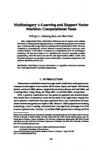
Figure 1. Schematic of level and stretched coordinates
a −b σ = a+ (z − ζ ) H
(3.2)
σ −a z = H +ζ a −b
(3.3)
(Figure 1) in which the vertical dimension is transformed from z, ranging from -h to ζ , to σ, ranging from b to a, where b and a are arbitrary constants. (Most models assume b=-1, a=0. ADCIRC assumes b=-1, a=1.) While ADCIRC uses the variable σ to represent the stretched vertical coordinate, a traditional “σ” coordinate system implies that the nodes are spaced uniformly over the vertical at any given horizontal location. ADCIRC does not carry this limitation, but rather nodes can be distributed over the vertical in any manner desired. Using the chain rule we can relate derivatives along level (z) surfaces to derivatives along the stretched (σ) surfaces: ∂ ∂x z
=
σ − b ∂ζ σ − a ∂h ∂ − + ∂x σ a − b ∂x z a − b ∂x z ∂z ∂
∂ ∂ σ − b ∂ζ σ − a ∂h ∂ = − + ∂y z ∂y σ a − b ∂y z a − b ∂y z ∂z
(3.4)
∂ a −b ∂ = ∂z H ∂σ
31
where for clarity, σ subscripts have been used on the horizontal derivatives computed along the stretched surfaces in Eqs. (3.4). Considerable discussion exists in the literature regarding the generation of spurious circulation due to the use of stretched vertical coordinates. Most of this attention has focused on problems arising from the baroclinic pressure gradient terms and to a lesser extent the lateral stress terms. In ADCIRC we apply the stretched coordinate system to all but the baroclinic pressure gradient terms resulting in the following transformed momentum equations: ∂u ∂u ∂u a − b ∂u +u +v + wσ − fv = ∂t ∂yσ H ∂σ ∂xσ −g
∂ [ζ + P s g ρ o − αη ] a − b ∂ + ∂x H ∂σ
τ zx − bx + mxσ ρo
∂v ∂v ∂v a − b ∂v +u +v + wσ + fu = ∂t ∂yσ H ∂σ ∂xσ −g
(3.5)
∂ [ζ + P s g ρ o − αη ] a − b ∂ τ zy + − by + m yσ ∂y H ∂σ ρ o
Note that the first term on the right hand side of each equation is not a function of depth and therefore horizontal derivatives in level coordinates are identical to horizontal derivatives in stretched coordinates. Introduction of the stretched coordinate system in the advection terms produces similar-looking advection terms in the stretched coordinate system, Eqs. (3.5), provided a stretched-coordinate, vertical velocity, wσ , is introduced that is related to the true vertical velocity by: σ − b ∂ζ σ − a ∂h σ − b ∂ζ σ − a ∂h σ − b ∂ζ wσ ≡ w − − u + − v + a − b ∂t a − b ∂x a − b ∂x a − b ∂y a − b ∂y
(3.6)
ADCIRC does not formally transform the lateral stress terms ( m x, m y ) in Eqs. (3.4) to obtain equivalent terms in Eqs. (3.5). Rather, the original lateral stress terms (along horizontal surfaces) are approximated as lateral stresses “along stretched surfaces”, i.e., m xσ ≡ m yσ
∂ ∂u ∂ ∂u El = lateral stress gradients along stretched surface El + ∂xσ ∂xσ ∂y σ ∂y σ
∂ ∂v ∂ ∂v ≡ El = lateral stress gradients along stretched surface El + ∂xσ ∂xσ ∂y σ ∂y σ
32
(3.7)
The generation of spurious circulation because of this assumption has also been discussed in the literature. ADCIRC uses the lateral stress gradient terms purely to dampen numerical noise in the solution and therefore assumes a lateral stress coefficient that is as small as possible. This should minimize the generation of spurious circulation by these terms. The weighted residual method is applied to Eqs. (3.5) by multiplying each term by a horizontal weighting function φ j and integrating over the horizontal computational domain Ω and then multiplying the result by a vertical weighting function ψ k and integrating over the vertical domain, Ζ . By constructing the grid so that the vertical nodes line up vertically beneath each horizontal node, the horizontal and vertical integrations can be performed independently. ∂u ,φ j ∂t − −
g
−
g
(
+
Ω
Ζ
u
∂u ∂xσ
+v
Ω
,ψ k
,ψ k Ω
+
a−b∂u + wσ ,φ j ∂yσ H ∂σ
(
+ Ζ
u
∂v ∂xσ
+v
Ω
Ω
,ψ k
+ Ζ
Ζ
Ω
,ψ k
a−b ∂ H ∂σ
)
a −b∂v + wσ ,φ j ∂yσ H ∂σ
m yσ , φ j
+
,ψ k Ω
Ω
Ζ
,ψ k
,ψ k Ω
fv,φ j
−
Ω
,ψ k
Ζ
τ zx ,φ j ρo
= Ζ
,ψ k Ω
(3.8) Ζ
Ζ
∂v
∂ [ζ + P s g ρ o − αη ] ,φ j ∂y
b y,φ j
+
,ψ k
m xσ , φ j
Ζ
)
∂u
∂ [ζ + P s g ρ o − αη ] ,φ j ∂x
b x, φ j
∂v ,φ j ∂t −
,ψ k
,ψ k Ω
fu,φ j
+ Ζ
a − b ∂ τ zy ,φ j H ∂σ ρ o
,ψ k Ω
Ω
,ψ k
= Ζ
(3.9) Ζ
Ζ
Horizontal integrations of each term in Eq. (3.8) are presented below (Eq. (3.9) is fully analogous) and are carried out using one of two basic integration rules as noted in the text. These rules are described in APPENDIX - BASIC CALCULATIONS ON LINEAR TRIANGLES: Horizontal integration of the transient term in Eq. (3.8) utilizes Rule 1: ∂u ,φ j ∂t
,ψ k Ω
= Ζ
A NE j 3
∂u j ∂t
,ψ k Ζ
33
Horizontal integration of the horizontal advection terms in Eq. (3.8) utilizes Rule 2 and assumes 1 3 1 3 the un-differentiated velocity terms are elementally averaged (i.e., u n ≡ ∑ u i and v n ≡ ∑ v i ): 3 i =1 3 i =1
(
u
∂u ∂xσ
+v
∂u ∂y σ
)
,φ j
,ψ k
NE j
∑
=
Ω
n =1
Ζ
An
∂u ∂u u n v n + ,ψ 3 ∂xσ n ∂yσ n k
Ζ
Horizontal integration of the vertical advection term in Eq. (3.8) utilizes Rule 1:
(
)
a −b ∂u ,φ j wσ H ∂σ
,ψ k
=
Ω
Ζ
A NE j a − b ∂uj ,ψ k wσ j ∂σ 3 Hj
Ζ
Horizontal integration of the Coriolis term in Eq. (3.8) utilizes Rule 1: fv,φ j
Ω
,ψ k
= Ζ
A NE j 3
fv j ,ψ k
Ζ
Horizontal integration of the combined barotropic pressure (i.e., the free surface elevation, atmospheric pressure and tidal potential) gradient term in Eq. (3.8) utilizes Rule 2: ∂ [ gζ + P s ρ o − α gη ] ,φ j ∂x
=
,ψ k Ω
Ζ
NE j
∂ [ζ + P s g ρ o − αη ] ,ψ k ∂x n
∑ A3 g n =1
n
Ζ
Horizontal integration of the vertical stress gradient term in Eq. (3.8) utilizes Rule 1: a − b ∂ τ zx ,φ j H ∂σ ρ o
=
,ψ k Ω
Ζ
A NE j a − b ∂ τ zx j ,ψ 3 H j ∂σ ρ o k
Ζ
Horizontal integration of the baroclinic pressure gradient terms in Eq. (3.8) utilizes Rule 2:
b x, φ j
Ω
,ψ k
= Ζ
NE j
∑ A3 b n =1
n
xn
,ψ k Ζ
Horizontal integration of the lateral stress gradient term in Eq. (3.8) initially utilizes integration by parts
34
m xσ , φ j
Ω
∂ ∂u ∂ ∂u + E E ,φ j l l ∂xσ ∂xσ ∂y σ ∂y σ
≡
,ψ k
Ζ
,ψ k Ω
Ζ
NE j ∂u ∂u ∂u ∂φ j ∂u ∂φ j = ∫ El φ + Γ − + Ω d d ,ψ k E j l ∑ ∫ ∂ ∂ ∂ y y y ∂ ∂ ∂ x x x 1 = n σ σ σ σ Ωn Γ n
NE j ∂u ∂u ∂u ∂φ j ∂u ∂φ j = ∫ El φ d + Γ − + j ∑ ∂y σ ∂y n Γ n ∂xσ ∂y σ n =1 ∂xσ ∂x
d Ω ∫ E l ,ψ k Ωn
Ζ
Ζ
where, Γ n = external boundary segment of element n . The term is further reduced by assuming that the lateral stresses are zero along all external boundary segments and by lumping the lateral stress coefficient
m xσ , φ j
Ω
NE j ∂u ∂φ j ∂u ∂φ j = − E l j ∑ A n + ,ψ k ∂xσ ∂x y y ∂ ∂ Ζ n =1 σ n
,ψ k
Ζ
Thus, following horizontal integration and multiplication by 3 A NE j , Eqs. (3.8) and (3.9) become: ∂u j ∂t
,ψ k
+ Ζ
− fv j ,ψ k
−
1 A NE j
1 A NE j
Ζ
=−
∑ A u
NE j
n
n =1
1
a −b ∂uj + ,ψ k wσ j ∂σ H j Ζ
∂ [ζ + P s g ρ o − αη ] ,ψ k ∂ x n
∑ A g n
n =1
NE j n =1
∂u ∂u ,ψ k + v n ∂ y ∂xσ n σ n
NE j
A NE j
∑ Anb x n,ψ k
n
− Ζ
3 A NE j
a −b H
+ Ζ
NE j ∂u ∂φ j ∂u ∂φ j E l j ∑ A n + ,ψ k ∂xσ ∂x ∂y σ ∂y n =1 n
35
j
Ζ
∂ ∂σ
Ζ
τ zx j ,ψ ρo k
(3.10) Ζ
∂v j ∂t
,ψ k
−
1
n
A NE j
Ζ
+ fu j ,ψ k
∑ A u
NE j
1
+
Ζ
=−
n =1
1
∑A b n
n =1
yn
∂v ∂v ,ψ k + v n ∂xσ n ∂y σ n
NE j
a −b ∂vj + ,ψ k wσ j ∂σ Hj Ζ
∂ [ζ + P s g ρ o − αη ] ,ψ k ∂y n
∑ A g n
A NE j
NE j
A NE j
n
n =1
,ψ k
− Ζ
3 A NE j
a −b H
+ Ζ
j
NE j ∂v ∂φ j ∂v ∂φ j E l j ∑ A n + ,ψ k ∂xσ ∂x ∂y σ ∂y n n =1
∂ ∂σ
Ζ
τ zy j ,ψ k ρ o
(3.11) Ζ
Ζ
A standard one-dimensional, Galerkin FEM discretization is used in the vertical, yielding the following integration rule,
ϒ,ψ k
σk σk ϒ k −1 ∫ ψ k −1ψ k d σ + ϒ k ∫ ψ kψ k d σ σ k −1 σ k −1 σk σ k +1 σ k +1 ≡ ϒ k −1 ∫ ψ k −1ψ k d σ + ϒ k ∫ ψ kψ k d σ + ϒ k +1 ∫ ψ k +1ψ k d σ z σ k −1 σ k −1 σk σ k +1 σ k +1 ϒ k ∫ ψ kψ k d σ + ϒ k +1 ∫ ψ k +1ψ k d σ σ k σk
In shorthand notation this can be written as: ϒ,ψ k
3
z
≡ ϒ k −1Inm k ,1 + ϒ k Inm k ,2 + ϒ k +1Inm k ,3 = ∑ ϒ k + m − 2 Inm k ,m m =1
where,
ψ k = vertical weighting function, =1 at node k, =0 at all other nodes, varies linearly between adjacent nodes k = 1 at the bottom k = NV at the free surface NV = number of nodes in the vertical
36
k = NV
1 < k < NV
k =1
σ σk 1 k σ − σ k −1 = d σ ψ ψ ψ kψ k d σ = k k −1 k ∫ ∫ 2 6 Inm k ,1 = σ σ k −1 k −1 0 Inm k ,2 = 2 ( Inm k ,1 + Inm k ,3 )
for k ≠ 1 for k = 1
σ σ k +1 1 k +1 σ −σ k ψ kψ k d σ = k +1 ψ k +1ψ k d σ = ∫ ∫ 2 6 Inm k ,3 = σ σk k 0
(3.12) for k ≠ NV for k = NV
Note, that the definition of the weighting/basis function ψ k reduces integration over the vertical domain Ζ to integration over only the two vertical elements containing node k, i.e., from node k − 1 to node k + 1 . Also, because the basis functions are linear in space, their derivatives are constant within an element and can be pulled out of elemental integrations. Vertical integration of the transient term in Eq. (3.10) yields ∂u j ∂t
∂u j ,k + m − 2 Inm k ,m ∂t m =1 3
=∑
,ψ k Ζ
Vertical integration of the horizontal advection terms in Eq. (3.10) yields 1
∑ A u
NE j
n
A NE j
n =1
n
∂u ∂u + v n ,ψ k ∂xσ n ∂y σ n =
1
Ζ
∑ ∑ A 3
A NE j m =1
NE j n =1
n
∂u ∂ u Inm k ,m u n + v n ∂y σ n ∂xσ n k + m−2
Vertical integration of the vertical advection term in Eq. (3.10) yields
37
a−b ∂u j ,ψ k wσ j ∂σ Hj
( ) ( )
a − b ∂u j = Ζ H j ∂σ
σk
wσ k -1,k
j ,k −1
∫
ψ kψ k −1 d σ + wσ j ,k
σk
∫
ψ kψ k d σ
σ k −1 σ k −1 σ k +1 σ k +1 a − b ∂u j d d σ σ + + ψ ψ ψ ψ wσ j ,k ∫ k k wσ j ,k +1 ∫ k k +1 H j ∂σ k ,k +1 σk σk
a − b ∂u j = wσ H j ∂σ k -1,k
(
+ 2 wσ j ,k −1
j ,k
) Inm
k ,1
(
∂u + j 2 wσ ∂σ k ,k +1
+ wσ j ,k
j ,k +1
) Inm
k ,3
where,
( ) ( ) ∂u j ∂σ
∂u j ∂σ
( ) ( )
≡ u j ,k −1 k -1, k
≡ u j ,k k , k +1
∂ψ k −1 ∂σ
∂ψ k ∂σ
( ) ( )
+ u j ,k k -1, k
+ u j ,k +1
k , k +1
∂ψ k ∂σ
∂ψ k +1 ∂σ
=
k -1, k
u j ,k − u j ,k −1 σ k − σ k −1
= k , k +1
u j ,k +1 − u j ,k σ k +1 − σ k
Vertical integration of the Coriolis term in Eq. (3.10) yields fv j ,ψ k
3
Ζ
= ∑ fv j ,k + m − 2 Inm k ,m m =1
Vertical integration of the barotropic pressure gradient term in Eq. (3.10) yields 1 ANE j
∂ [ζ + P s g ρ o − αη ] An g ,ψ k ∑ ∂x n =1 n NE j
= Ζ
NE j
1 ANE j
∂ [ζ + P s g ρ o − αη ] LVn k ∂x n
∑A g n
n =1
where σk − ψ k d σ = σ k σ k −1 ∫ 2 σ k −1 σ k +1 σ k +1 − σ k −1 LVn k ≡ ∫ ψ k d σ = 2 σ k −1 σ k +1 σ k +1 − σ k ∫ ψ k dσ = 2 σ k
k = NV
1 < k < NV
k =1
38
(3.13)
Vertical integration of the baroclinic pressure gradient term in Eq. (3.10) yields 1
NE j
∑A b n
A NE j
n =1
xn
=
,ψ k Ζ
NE j Inm k ,m ∑ A nb x n ∑ A NE j m =1 n =1 k + m−2 1
3
Vertical integration of the lateral stress terms in Eq. (3.10) yields NE j ∂u ∂φ j ∂u ∂φ j E l j ∑ A n + ,ψ k ∂xσ ∂x ∂y σ ∂y n =1 n
3 A NE j
Ζ
NE j ∂u ∂φ j ∂u ∂φ j = + Inm k ,m An ∑ E l j∑ ∂y σ ∂y A NE j m =1 n =1 ∂xσ ∂x n k + m−2 3
3
The vertical stress gradient term in Eq. (3.10) is initially integrated by parts, yielding
a −b H j
∂ ∂σ
τ zx j ,ψ ρo k
Ζ
a − b τ sx j = ρ Hj o
a − b τ bx j − ρ k = NV Hj o
a − b τ zx j ∂ψ k − , ρ o ∂σ k =1 H j
Ζ
where the free surface stress, τ sx j (applied only for k=NV) and bottom stress τ bx j (applied only for k=1) have been introduced. Expressing the vertical stress in terms of the vertical gradient of velocity in the remaining integral term, yields:
τ zx j ∂ψ k , ρ o ∂σ
= Ζ
( ) a −b Hj
∂u j ∂ψ k E z j ∂σ , ∂σ
= Ζ
σk σk ∂ψ k ∂ψ k u j ,k −1 ∂ψ k −1 + u j ,k ∂σ E z j ,k −1 ∫ ψ k −1 d σ + E z j ,k ∫ ψ k d σ σ σ ∂ ∂ k −1,k k −1,k k −1,k a −b σ k −1 σ k −1 σ σ k +1 k +1 H j ∂ψ k ∂ψ k +1 ∂ψ k + u j ,k + u j ,k +1 E z j ,k ∫ ψ k d σ + E z j ,k +1 ∫ ψ k +1 d σ σ σ σ ∂ ∂ ∂ k ,k +1 k ,k +1 k ,k +1 σk σk or in shorthand notation τ zx j ∂ψ k , ρ o ∂σ
a −b 3 = ∑ u j ,k + m − 2 KVnm j ,k ,m H j m =1 Ζ
39
where σk σk ∂ψ k −1 ∂ψ k d d + σ σ ψ ψ k −1 k E z j ,k ∫ ∂σ k −1,k ∂σ k −1,k E z j ,k −1 ∫ σ σ k −1 k −1 σk σk = − ∂ψ k ∂ψ k E z j ,k −1 ∫ ψ k −1 d σ + E z j ,k ∫ ψ k d σ KVnm j ,k ,1 = ∂σ k −1,k ∂σ k −1,k σ k −1 σ k −1 + = − E z j ,k E z j ,k −1 for k ≠ 1 2 (σ k − σ k −1) for k = 1 0 KVnm j ,k ,2 = − ( KVnm k ,1 + KVnm k ,3 ) σ k +1 σ k +1 ∂ψ k +1 ∂ψ k d d σ σ + ψ ψ k k +1 E z j ,k +1 ∫ ∂σ k ,k +1 ∂σ k ,k +1 E z j ,k ∫ σ σ k k σ k +1 σ k +1 = − ∂ψ k ∂ψ k d d σ σ + ψ ψ k k +1 ∂σ ∂σ E z j ,k ∫ E z j ,k +1 ∫ KVnm j ,k ,3 = k ,k +1 k ,k +1 σk σk + = − E z j ,k +1 E z j ,k for k ≠ NV 2 (σ k +1 − σ k ) for k = NV 0
(3.14)
ADCIRC utilizes a generalized slip formulation for the bottom stress term:
τ bx j = K slip j u j; ρo
τ by j = K slip j v j ρo
where, K slip j → ∞
= no slip bottom boundary condition
K slip j = constant ,
= linear slip bottom boundary condition, ( K slip j= linear drag coefficent)
K slip j = C d u 2j + v 2j , = quadratic slip bottom boundary condition, ( C d = quadratic drag coefficent) In final form, the vertical stress gradient term is:
40
a − b ∂ τ zx j ,ψ k H j ∂σ ρ o
Ζ
a − b τ sx j = ρ Hj o
a −b a−b − u j k =1K slip j − k = NV Hj Hj
41
2
3
∑u m =1
j ,k + m−2
KVnm j ,k ,m
Thus, following vertical integration Eqs. (3.10), (3.11) become: 1 3 NE j ∂ u ∂ u ∂u j ,k + m − 2 Inm k ,m + + ∑ u v A ∑ n n n ∂y Inm k ,m ∂t A NE j m =1 n =1 ∂xσ n m =1 σ n k + m − 2 3
∑
a − b ∂u j ∂u j + + + + wσ j ,k +1 Inm k ,3 2 w w σ j , k −1 2 wσ j , k Inm k ,1 σ j ,k ∂σ k ,k +1 H j ∂σ k -1,k 3 1 NE j ∂ [ζ + P s g ρ o − αη ] − ∑ f v j ,k + m − 2 Inm k ,m = − LVn k ∑ A n g ∂x m =1 A NE j n =1 n
(
)
(
)
(3.15)
2
a − b τ sx j + ρ Hj o
a −b a −b 3 − u j k =1K slip j − ∑ u j ,k + m − 2 KVnm j ,k ,m k = NV Hj H j m =1 1 3 NE j 3 3 NE j ∂u ∂φ j ∂u ∂φ j E l j ∑ A n + − − Inm k ,m ∑ ∑ Anb x n Inm k ,m A ∑ y y ∂ ∂ x x ∂ ∂ A NE j m =1 n =1 m n = = 1 1 σ NE j σ k + m−2 n k + m − 2 1 3 NE j ∂ v ∂ v ∂v j ,k + m − 2 Inm k ,m + + ∑ u v A ∑ n n n ∂y Inm k ,m ∂t A NE j m =1 n =1 ∂xσ n m =1 σ n k + m − 2 3
∑
a − b ∂v j ∂v j + + + + wσ j ,k +1 Inm k ,3 w w 2 σ j , k −1 2 wσ j , k Inm k ,1 σ j ,k ∂σ k ,k +1 H j ∂σ k -1,k
(
3
+ ∑ f u j ,k + m − 2 Inm k ,m = − m =1
a − b τ sy j + ρ Hj o −
)
1 A NE j
NE j
(
)
∂ [ζ + P s g ρ o − αη ] LVn k ∂y n
∑ A g n
n =1
a −b a −b − v j k =1K slip j − Hj Hj k = NV
2
(3.16)
3
∑v
j ,k + m − 2
KVnm j ,k ,m
m =1
NE j 3 3 NE j ∂v ∂φ j ∂v ∂φ j E l j ∑ A n − + Inm k ,m ∑ ∑ Anb y n Inm k ,m A ∑ ∂xσ ∂x ∂ ∂ y y A NE j m =1 n =1 1 1 = = m n NE σ j k + m−2 n k + m − 2 1
3
Equations (3.15), (3.16) present the spatially discretized solution for velocity at horizontal node j and vertical node k used by ADCIRC 3D. These equations are discretized in time using a two time level scheme at the present (s) and future (s+1) time levels as described below: u j ,k + m−2 − u j ,k + m−2 Inm k ,m ∑ ∆t m =1 3
Transient term:
s +1
s
42
∑ ∑ A NE j
3
1
Horizontal advection:
A NE j m =1
n
n =1
s ∂ u s s s ∂u Inm k ,m u n + v n ∂y σ n ∂xσ n k + m−2
Vertical advection:
( )
a − b ∂u sj s H j ∂σ
(w
σ j , k −1
∑ f α v 1
s +1 j ,k + m − 2
m =1
Free surface stress:
Bottom stress:
)
+ 2 wσ j ,k Inm k ,1 + s
k -1, k
3
Coriolis:
s
( ) s
∂u j ∂σ
( 2w
s
σ j ,k
k , k +1
+ wσs j ,k +1 Inm k ,3
)
+ (1 − α 1) v sj ,k + m − 2 Inm k ,m
s a − b τ ssx+1j τ sx j + 2 H sj+1 ρ o H sj ρ o k = NV
( a − b ) K slip j α 2 us +j1
s +1
s
Hj
+
(1 − α ) u H 2
s j
s j
k =1
Barotropic pressure gradient: s s +1 An g ∂[ζ + P s g ρ o − αη ] + g ∂[ζ + P s g ρ o − αη ] LVn k ∑ ∂x ∂x ANE j n =1 2 n
1
NE j
Vertical stress:
3
m =1
( a − b ) ∑ α 3 2
Baroclinic pressure gradient:
Lateral stress:
3
3
s +1
u j ,k + m−2
(H )
s +1 2 j
+ (1 − α 3 )
NE j s Inm k ,m ∑ A nb x n ∑ A NE j m =1 n =1 k + m−2 3
1
NE j
s
∂φ j
∑ E ∑ A ∂∂xuσ ∂x
A NE j m =1
s lj
s u j ,k + m − 2 s KVnm j ,k ,m s 2 (H j)
n
n =1
+
s ∂u ∂φ j Inm k ,m ∂y σ ∂y n k + m−2
Substituting these into Eqs. (3.15) and (3.16), multiplying by ∆t and grouping velocities at time levels s+1 and s yields: 43
3
∑u
s +1 j ,k + m − 2
m =1
3
Inm k ,m − ∆t ∑ f α v
s +1 1 j ,k + m−2
m =1
+ α 3 ∆t
( )∑ a −b s +1
Hj
2
3
u
s +1 j ,k + m −2
( a − b ) ∆tα 2 K sslip j u sj+1 k =1 Inm k ,m + s +1 H j
KVnm
s j ,k ,m
m =1
=
3
∑u
s j ,k + m−2
m =1
3
s Inm k ,m + ∆t ∑ f (1 − α 1) v j ,k + m − 2 Inm k ,m
( )
( a − b ) ∆t (1 − α 2 ) K sslip j u sj k =1 − (1 − α 3 ) ∆t a − b − s s Hj Hj −
∆t
∑∑ A 3
A NE j m =1
NE j n =1
n
( )
−
−
(
)
wσ j ,k −1 + 2wσs j ,k Inm k ,1 + s
k -1, k
s ∆t ( a − b ) τ ssx+1j τ sx j + 2 H sj+1ρ o H sj ρ o
∆t A NE j
NE j
∑ n =1
2
3
∑u
s j ,k + m − 2
s
KVnm j ,k ,m
m =1
∂ us s s ∂u Inm k ,m + u ns v n ∂xσ n ∂y σ n k + m−2
a − b ∂u sj − ∆t s H j ∂σ +
m =1
( ) s
∂u j ∂σ
( 2w
s
σ j ,k
k , k +1
+ wσs j ,k +1 Inm k ,3
)
k = NV
s s +1 ∂[ζ + P s g ρ o − αη ] An g ∂[ζ + P s g ρ o − αη ] LVn k +g 2 ∂x ∂x n
NE j 3∆t 3 s NE j ∂u s ∂φ j ∂u s ∂φ j s − + Inm Inm k ,m b An A k ,m ∑ ∑ n xn ∑ E l j∑ y y ∂ ∂ x x ∂ ∂ A NE j m =1 n =1 A NE j m =1 n =1 σ σ k + m−2 n k + m−2 ∆t
3
44
(3.17)
3
∑v
s +1 j ,k + m−2
m =1
3
Inm k ,m + ∆t ∑ f α u
s +1 1 j ,k + m − 2
m =1
+ α 3 ∆t
( )∑ a −b s +1
Hj
2
3
v
s +1 j ,k + m−2
( a − b ) ∆tα 2 K sslip j v sj+1 k =1 Inm k ,m + s +1 H j
KVnm
s j ,k ,m
m =1
=
3
∑v
s j ,k + m−2
m =1
3
s Inm k ,m − ∆t ∑ f (1 − α 1) u j ,k + m − 2 Inm k ,m
( )
( a − b ) ∆t (1 − α 2 ) K sslip j v sj k =1 − (1 − α 3 ) ∆t a − b − s s Hj Hj −
∆t
∑ ∑ A 3
A NE j m =1
NE j n =1
n
m =1
2
3
∑v
s j ,k + m − 2
s
KVnm j ,k ,m
m =1
∂ vs s s ∂v Inm k ,m + u ns v n ∂xσ n ∂y σ n k + m−2
( )
a − b ∂v sj − ∆t s H j ∂σ
(
)
wσ j ,k −1 + 2wσs j ,k Inm k ,1 + s
k -1, k
( ) s
∂v j ∂σ
( 2w
s
σ j ,k
k , k +1
+ wσs j ,k +1 Inm k ,3
)
s ∆t ( a − b ) τ ssy+1j τ sy j + + 2 H sj+1ρ o H sj ρ o k = NV
−
−
∆t A NE j
NE j
∑ n =1
s s +1 ∂[ζ + P s g ρ o − αη ] An g ∂[ζ + P s g ρ o − αη ] LVn k +g 2 ∂y ∂y n
NE j 3∆t 3 s NE j ∂v s ∂φ j ∂v s ∂φ j s + − Inm k ,m b Inm An A k ,m ∑ ∑ n yn ∑ E l j∑ y y ∂ ∂ x x ∂ ∂ A NE j m =1 n =1 A NE j m =1 n =1 σ σ k + m−2 n k + m−2 ∆t
3
45
(3.18)
Prior to obtaining the 3D velocity solution in ADCIRC, a complex velocity, q, is defined as q ≡ u + iv
i ≡ −1
where
and Eqs. (3.17) and (3.18) are rewritten so that the x momentum equation is the real part and the y momentum equation is the imaginary part of a single complex equation: 3
∑q m =1
s +1 j ,k + m −2
3
Inm k ,m + i∆t f α 1∑ q
+ α 3 ∆t
( )∑ a −b s +1
Hj
2
m =1
3
q
m =1
s +1 j ,k + m−2
s +1 j ,k + m−2
KVnm
( a − b ) ∆tα 2 K sslip j s +1 q j Inm k ,m + s +1 k =1 H j
s j ,k ,m
=
3
∑q m =1
s j ,k + m− 2
3
s Inm k ,m − i∆t f (1 − α 1) ∑ q j ,k + m − 2 Inm k ,m
( )∑
( a − b ) ∆t (1 − α 2 ) K sslip j s q j − (1 − α 3 ) ∆t a − b − s s k =1 Hj Hj −
∆t
∑ ∑ A 3
A NE j m =1
NE j n =1
2
3
m =1
m =1
s
q j ,k + m − 2 KVnm sj ,k ,m
s ∂ qs s s ∂q Inm k ,m + u v n n n ∂xσ n ∂y σ n k + m−2
( )
s a − b ∂q j − ∆t s H j ∂σ
(
s
( ) s
)
wσ j ,k −1 + 2wσ j ,k Inm k ,1 + s
k -1, k
∂q j ∂σ
( k , k +1
s + 2wσ j ,k wσ j ,k +1 Inm k ,3 s
)
τ ssy+1j ∆t ( a − b ) τ ssx+1j τ ssy j τ ssx j + H sj+1ρ o + H sj ρ o + i H sj+1ρ o + H sj ρ o 2 k = NV s s +1 ∂[ζ + P s g ρ o − αη ] An g ∂[ζ + P s g ρ o − αη ] LVn k − +g ∑ ∂x ∂x A NE j n =1 2 n
−
∆t
NE j
i∆t
NE j
A NE j
∑ n =1
s +1 s An g ∂[ζ + P s g ρ o − αη ] + g ∂ ζ + P s g ρ o − αη LVn k 2 ∂y ∂y n
−
NE j s s Inm k ,m ∑ A n b x n + ib y n ∑ A NE j m =1 n =1 k + m−2
−
NE j ∂q s ∂φ j ∂q s ∂φ j E ls j ∑ An + Inm k ,m ∑ ∂xσ ∂x y y ∂ ∂ A NE j m =1 n =1 σ n k + m − 2
∆t
3∆t
3
(
)
3
46
(3.19)
Re-arranging and consolidating terms yields the form of the 3D momentum equations solved in ADCIRC: 3
(1 + i∆t f α 1) ∑ q sj+,k1+m−2 Inm k ,m + α 3 ∆t m =1
( )∑ 2
a−b H
s +1 j
3
m =1
s +1
q j ,k + m−2 KVnm sj ,k ,m
( a − b ) ∆tα 2 K s slip j q s +1 + s +1 j k =1 Hj 3
{
}
= ∑ (1 − i∆t f (1 − α 1) ) q sj ,k + m−2 − ∆t[ladvec + lstress + bcpg ] j ,k + m −2 Inm k ,m m =1
(3.20)
( a − b ) ∆t (1 − α 2 ) K s slip j qs − ∆t vadvec j ,k − ∆t btpg j LVn k − (1 − α 3 ) ∆t vstress j ,k − s j k =1 Hj s
τ ssy+1j ∆t ( a − b ) τ ssx+1j τ ssy j τ ssx j + 2 H sj+1ρ o + H sj ρ o + i H sj+1ρ o + H sj ρ o k = NV
where,
ladvec j ,k ≡
1 A ∑ A NE j
NE j n =1
s ∂ qs s s ∂q n u n + v n ∂y σ n ∂xσ n k
( )
s a − b ∂q j vadvec j ,k ≡ s H j ∂σ
bcpg j ,k ≡
1 A ∑ A ( b NE j
n
NE j n =1
s xn
(w
s
σ j , k −1
)
+ 2 wσ j ,k Inm k ,1 + s
k -1, k
+ ib sy n
)
( ) s
∂q j ∂σ
( 2w
s
σ j ,k
+ wσ j ,k +1
k , k +1
k
∂[ζ + P g ρ − αη ]s ∂[ζ + P g ρ − αη ]s +1 s s o o + x x ∂ ∂ NE j g An 1 btpg j ≡ ∑ s A NE j n =1 2 ∂[ζ + P s g ρ − αη ] ∂[ζ + P s g ρ − αη ]s +1 o o +i + ∂y ∂y n
47
s
)
Inm k ,3
lstress j ,k
∂q ∂φ 3E ≡ A ∑ A ∂xσ ∂x s NE j lj
NE j
vstress
s j ,k
≡
s
n
n =1
( )∑ a −b H
s j
2
3
m =1
j
s ∂q ∂φ j + ∂y σ ∂y
n
k
s
q j ,k + m − 2 KVnm sj ,k ,m
Eq. (3.20) has a matrix structure, although due to the specific formulation that was used to obtain this equation, the matrix is uncoupled in the horizontal direction and is tri-diagonal in the vertical direction. Thus, Eq. (3.20) is solved separately for each horizontal node j. Symbolically, Eq. (3.20) can be written as: Mq = F r
where, M = complex tridiagonal matrix q = complex solution vector for velocity F r = complex forcing vector
M consists of:
( )
(1 + i∆tα 1 f ) Inm k ,1 + α 3 ∆t M ( k , k − 1) = 0 (1 + i∆tα 1 f ) Inm k ,2 + α 3 ∆t M (k, k ) = (1 + i∆tα 1 f ) Inm k ,2 + α 3 ∆t (1 + i∆tα 1 f ) Inm k ,3 + α 3 ∆t M ( k , k + 1) = 0
a −b H
2
( ) ( ) ( ) a −b H
2
s +1
a −b
for k ≠ 1
s
KVnm j ,k ,2
2
Hj
H
for k = 1
s +1 j
a −b
for k ≠ 1
s
KVnm j ,k ,1
s +1 j
KVnm
s j , k ,2
( a − b ) ∆tα 2 K sslip j + s +1 H j
for k = 1
2
s +1 j
s
KVnm j ,k ,3
for k ≠ NV for k = NV
and Fr consists of:
48
3 ∑ (1 − i∆t f (1 − α 1) ) q sj ,k + m − 2 − ∆t[ladvec + lstress + bcpg ] j ,k + m − 2 Inm k ,m m=2 s = − ∆t vadvec j ,k − ∆t btpg j LVn k − (1 − α 3 ) ∆t vstress j ,k ( a − b ) ∆t (1 − α 2 ) K s slip j qs − s j ,k Hj
{
}
{
for k = 1
}
3 s ∑ (1 − i∆t f (1 − α 1) ) q j ,k + m − 2 − ∆t[ladvec + lstress + bcpg ] j ,k + m − 2 Inm k ,m F r ( k ) = m =1 − ∆t vadvec − ∆t btpg LVn − (1 − α ) ∆t vstress s 3 k j j ,k j ,k 2 1 − i∆t f (1 − α 1) ) q sj ,k + m − 2 − ∆t[ladvec + lstress + bcpg ] j ,k + m − 2 Inm k ,m ( ∑ m =1 s = − ∆t vadvec j ,k − ∆t btpg j LVn k − (1 − α 3 ) ∆t vstress j ,k τ ssy+1j ∆t ( a − b ) τ ssx+1j τ ssy j τ ssx j s +1 + s + i s +1 + s + 2 H j ρ o H j ρ o H j ρ o H j ρ o
{
for k ≠ 1, NV
}
49
for k = NV
4.0 VERTICAL VELOCITY
The vertical component of velocity is obtained in ADCIRC by solving the 3D continuity equation ∂u ∂v = − + ∂z ∂x z ∂y z ∂w
(4.1)
for w after u and v have been determined from the solution of the 3D momentum equations. In Eq. (4.1), the subscript “z” has been added to the horizontal derivatives to emphasize that these derivatives are evaluated along level coordinate surfaces. Eq. (4.1) is solved subject to the freesurface and bottom kinematic boundary conditions: ws =
∂ζ ∂ζ ∂ζ +u s +v s ∂t ∂y z ∂x z
wb = −u b
∂h ∂x z
−v b
∂h ∂y z
at z = ζ
(4.2)
at z = -h
(4.3)
where us, vs, ws are the velocity components at the free surface (z=ζ) and ub, vb, wb are the velocity components at the bottom (z=-h) assuming a slip condition is applied there. Eq. (4.1) is discretized in horizontal space as: ∂w ,φ ∂z j
=− Ω
∂u ∂x z
,φ j
− Ω
∂v ,φ j ∂y z
(4.4) Ω
The horizontal integration utilizes Rule 1 for the left side and Rule 2 for the right side (these rules are described in APPENDIX - BASIC CALCULATIONS ON LINEAR TRIANGLES). After multiplication by 3 A NE j , Eq. (4.4) becomes:
∂ wj ∂z
=−
NE j 1 ∂u An A NE j ∑ n =1 ∂x z
+ ∂ v ∂y n
z
(4.5)
n
Eq. (4.5) is discretized over the vertical using a simple finite-difference for the left side and centering the right side:
50
NE j 1 ∂ u ∂ v ∂ u ∂ v w j ,k − w j ,k −1 =− A n + + + 2 A NE j ∑ z k − z k −1 n =1 ∂x z n ∂y z n k ∂x z n ∂y z n k −1
(4.6)
Eq. (4.6) can be written in terms of the stretched coordinate system as: ∂ u ∂ v − + ∂xσ n ∂y σ n k ∂ζ − a ∂H a − b ∂u j σ k + + ∂x n a − b ∂x n H j ∂σ k + ∂ζ + σ k − a ∂H a − b ∂v j ∂ σ ∂ − ∂ y a b y NE j n n H j 1 w j ,k − w j ,k −1 a − b k = 2 A ∑ An NE j n=1 σ k − σ k −1 H j ∂ u ∂ v + − y ∂ x ∂ σ σ n k −1 n ∂ζ σ k −1 − a ∂H a − b ∂u j + + ∂x n a − b ∂x n H j ∂σ k −1 ∂ζ σ k −1 − a ∂H a − b ∂v j + + ∂y n a − b ∂y n H j ∂σ k −1
(4.7)
The subscript “σ” indicates that the horizontal derivatives in (4.7) are evaluated along stretched coordinate surfaces. Discretizing the vertical derivative of horizontal velocity as:
∂u = ∂u ∂σ ∂σ j
j
k
k −1
u j ,k − u j ,k −1 = σ k − σ k −1
and re-arranging yields:
51
(σ k − σ k −1) H j ∂ u ∂ v ∂ u ∂ v + − + + 2 ( a − b ) ∂xσ n ∂y σ n ∂xσ n ∂y σ n k k −1 σ k + σ k −1 NE j −a 1 ∂ζ ∂H 2 w j ,k = w j ,k −1 + A ∑ An + (4.8) + ( u j ,k − u j ,k −1) NE j n =1 ∂ − ∂ x a b x n n σ k + σ k −1 − a ∂H + ∂ζ + 2 ( v j ,k − v j ,k −1) ∂y a −b n ∂y n
Eq. (4.3) is used to determine w j ,1 ; Eq. (4.8) can then be solved recursively for k=2, 3, … up to the surface. (Notice that the vertical differences of horizontal velocity in Eq. (4.8) are evaluated at node j only.) As discussed by Luettich et al. (2002) and Muccino et al. (1997), the result obtained for the vertical velocity at the free surface from Eq. (4.8), w j ,k = surface , may not match the free surface boundary condition, w j , s , as specified in Eq. (4.2). This discrepancy is due to error in local fluid mass conservation, (Luettich et al., 2002). ADCIRC attempts to optimally correct the vertical velocity obtained from Eq. (4.8) using an adjoint approach. This results in a correction to Eq. (4.8) that is linear over the depth:
ajoint corrected
w j ,k
W f σ −b 2 + a −b = w j ,k + ( w j , s − w j ,k = surface ) H 2W f + 1 H 2
(4.9)
In Eq. (4.9), Wf weights the relative importance of satisfying continuity in the interior of the fluid vs satisfying the free surface boundary condition in the adjoint equation. Setting Wf =0 forces the corrected vertical velocity to exactly satisfy the free surface and bottom boundary conditions. Setting Wf to be large (e.g., Wf ~100) adds a uniform correction to the vertical velocity solution that is equal to half the surface boundary error. ADCIRC uses a default value of Wf =0.
52
5.0 SPERHICAL COORDINATE FORMULATION
ADCIRC solves the spherical governing equations by transforming these equations into an equivalent set of equations in Cartesian coordinates using a standard cylindrical projection. Applying the hydrostatic and Bousinesque approximations and assuming the radius of the Earth is much greater than the thickness of the ocean, the 3D equations in spherical coordinates (λ,φ, z) are: (e.g., Haidvogel and Beckmann, 1999) Continuity r ∇ ⋅u =
1 ∂u 1 ∂ ( v cos φ ) ∂w 2 w + + + =0 R cos φ ∂λ R cos φ ∂φ ∂z R
(5.1)
Horizontal Momentum du g ∂ [ζ + P s g ρ o − αη ] ∂ τ zλ uv tan φ = fv − + − bλ + mλ + dt R cos φ ∂λ ∂z ρ o R
(5.2)
u 2 tan φ dv g ∂ [ζ + P s g ρ o − αη ] ∂ τ zφ = − fu − + − + − b φ mφ dt R ∂φ ∂z ρ o R
(5.3)
where R = 6.3782064x10 6 m, mean radius of the Earth λ , φ = longitude, latitude d u ∂ ∂ v ∂ ∂ = + + +w dt ∂t R cos φ ∂λ R ∂φ ∂z ∂v τ zλ , τ zφ = ∂u , Ez Ez ∂z ∂z ρo ρo m λ , mφ ≡ b λ , bφ ≡
1
( R cos φ )
2
g ∂ R cos φ ∂λ
∂ ∂u 1 ∂ ∂u El , El + ∂λ ∂λ R 2 ∂φ ∂φ
∫
ζ
z
( ρ − ρ o ) dz, ρo
g ∂ R ∂φ
∫
ζ
z
1
( R cos φ )
2
∂ ∂v 1 ∂ ∂v El El + ∂λ ∂λ R 2 ∂φ ∂φ
( ρ − ρ o ) dz ρo
and other variables are as defined in Section 3. Using a standard, orthogonal cylindrical projection centered at (λo, φo): 53
x=R ( λ − λ o ) cos φ o
(5.4)
y = Rφ
Derivatives are evaluated using the chain rule: ∂ ∂ ∂x ∂ ∂y ∂ = + =R cos φ o ∂λ ∂x ∂λ ∂y ∂λ ∂x ∂ ∂ ∂x ∂ ∂y ∂ = + =R ∂φ ∂x ∂φ ∂y ∂φ ∂y
Substituting for the derivatives in the spherical coordinate system with those in the Cartesian system gives a transformed set of spherical equations: Continuity ∂u ∂v ∂w v tan φ 2w r ∇ ⋅u = S p + + + + =0 ∂x ∂y ∂z R R
(5.5)
Horizontal Momentum ∂ [ζ + P s g ρ o − αη ] ∂ τ zx du uv tan φ = fv − g S p + − bx + mx + dt ∂x ∂z ρ o R
(5.6)
∂ [ζ + P s g ρ o − αη ] ∂ τ zy u 2 tan φ dv = − fu − g + − by + my − dt ∂y ∂z ρ o R
(5.7)
where Sp≡
cos φ o = spherical coordinate correction factor cos φ
54
(5.8)
d ∂ ∂ ∂ ∂ = +uS p +v + w dt ∂t ∂x ∂y ∂z ∂v τ zx , τ zy = ∂u , Ez Ez ∂z ∂z ρo ρo m x, m y ≡ S p
2
b x, b y ≡ g S p
∂ ∂u ∂ ∂u ∂v ∂ ∂v 2 ∂ El + El , S p El + El ∂x ∂x ∂y ∂y ∂x ∂x ∂y ∂y
∂ ζ ( ρ − ρ o) ∂ ζ ( ρ − ρ o) , dz g dz ∂x ∫z ∂y ∫z ρo ρo
A simple scaling analysis suggests that it may be permissible to drop the final two terms in Eq. (5.5) and the final terms in Eqs. (5.6) and (5.7), provided we avoid the regions near the poles where tan φ approaches infinity. This limitation is consistent with the singularity at the poles inherent in the original equations, Eqs. (5.1) - (5.3), and in the cylindrical mapping. Thus it does not appear to impose significant additional restrictions on the applicability of the governing equations. Dropping these terms simplifies the transformed spherical governing equations to: Continuity ∂u ∂v ∂w r ∇ ⋅u = S p + + =0 ∂x ∂y ∂z
(5.9)
Horizontal Momentum ∂ [ζ + P s g ρ o − αη ] ∂ τ zx ∂u ∂u ∂u ∂u + u S p + v + w − fv = − g S p + − bx + mx ∂t ∂x ∂y ∂z ∂x ∂z ρ o
(5.10)
∂ [ζ + P s g ρ o − αη ] ∂ τ zy ∂v ∂v ∂v ∂v + u S p + v + w + fu = − g + − by + my ∂t ∂x ∂y ∂z ∂y ∂z ρ o
(5.11)
These equations are identical to their Cartesian counterparts with the exception that spatial derivatives with respect to the x coordinate direction are multiplied by the spherical coordinate correction factor, Sp, defined in Eq. (5.8). Consequently, Eqs. (5.9) - (5.11) comprise a generalized set of equations that allows ADCIRC to function using either a Cartesian horizontal grid (by setting Sp = 1) or a longitude, latitude horizontal grid (by converting the longitude and latitude values into equivalent linear coordinate values, Eq. (5.4), and evaluating Sp, Eq. (5.8)).
55
The velocity in Eqs. (5.9) - (5.11) is aligned with the original coordinate reference frame (e.g., for the spherical coordinates (u, v, w) are aligned with (λ,φ, z)) and therefore it is not necessary to transform the velocities to a different coordinate system. Vertical integration of Eqs. (5.9) - (5.11) is identical to integration of the Cartesian equations. Thus, the two-dimensional, vertically-integrated equations are identical to their Cartesian counterparts, except that spatial derivatives with respect to the x coordinate direction are multiplied by Sp.
56
6.0 LATERAL BOUNDARY CONDITIONS
Elevation specified boundary condition –ADCIRC 2DDI and 3D An elevation specified boundary condition is implemented by zeroing out all off diagonal terms in the row corresponding to each elevation boundary node in the GWCE, Eq. (1.17), and setting the on diagonal term in that row equal to the root mean square value of all of the other diagonal terms in the GWCE matrix (to maintain matrix conditioning). The right side vector entry corresponding to each elevation specified boundary node is set equal to the specified elevation multiplied by the root mean square value mentioned previously. Symmetry is maintained in the left side matrix by zeroing out the off diagonal terms in the column corresponding to each elevation boundary node. To allow this, each off diagonal term in the column corresponding to an elevation boundary node is multiplied by the elevation boundary value and then subtracted from the right side vector of the corresponding equation.
Specified flux boundary condition –ADCIRC 2DDI ADCIRC allows the specification of boundary conditions consisting of normal flux per unit width (e.g., zero flux across land boundary segments and nonzero flux across river boundary segments). These normal fluxes can be applied as either natural or essential boundary conditions and the user may specify whether the tangential velocity along these boundaries is set to zero or computed assuming free slip along the boundary. The specified normal flux per unit width is inserted into the boundary integral term that appears in the right side of the GWCE, Eq. (1.17), at each normal flux boundary node. (The convention used in ADCIRC for inputting normal flux per unit width is that flux into the domain is positive and flux out of the domain is negative. Therefore, the sign must be changed on the normal flux prior to using it in the GWCE since the derivation of this equation assumes that a positive flux is in the direction of the outward pointing normal.) If the normal flux is applied as a natural boundary condition, no modifications are made to the momentum equations. If the normal flux is applied as an essential boundary condition, the depth-average normal velocity, UN, is forced to be equal to the normal flux per unit width divided by the local depth and multipled by –1 (to maintain the convention that UN is positive in the direction of the outward pointing normal). Further details of the implementation of the essential normal flux boundary condition in ADCIRC are presented below. At any node in the horizontal, the momentum equations solved in ADCIRC 2DDI have the structure:
AUV 1 − AUV 2 U F x = AUV 2 AUV 1 V F y
(6.1)
where AUV1, AUV2 are the matrix entries computed from the finite element assembly process, and Fx, Fy comprise the right side forcing vector. At flux specified boundary nodes, the 57
equations are rotated into a normal - tangential coordinate system. The normal and tangential velocities, UN and UT, are defined as the dot product of the velocity vector and the normal and tangential unit vectors, Nˆ = ( N x, N y ) and Tˆ = (T x, T y ) : UT x + VT y = U T UN x + VN y = U N
(6.2)
( Nˆ and Tˆ are defined in the APPENDIX.) At specified normal flux boundary nodes the ymomentum equation in (6.1) is replaced by the expression for the normal velocity in (6.2) and the x-momentum equation is replaced by the tangential momentum equation formed by multiplying the x-momentum equation (6.1) by Tx and adding the y-momentum equation (6.1) multiplied by Ty. Since Tx = Ny and Ty = -Nx (see APPENDIX), the resulting system is:
AUV 1 N y − AUV 2 N x − AUV 2 N y − AUV 1N x U F x N y − F y N x = Nx Ny UN V
(6.3)
The left side matrix in (6.3) does not have the symmetry of the original equations, (6.1). This can be recovered by adding the tangential momentum equation to the normal equation multiplied by AUV2 and dividing the result by AUV1: F x N y − F y N x + AUV 2 U N N y − N x U AUV 1 = V N x N y UN
(6.4)
For the case that the tangential flux is also specified (e.g., equal to zero), the right side of the first equation in (6.4) is replaced by UT.
Zero normal velocity gradient boundary condition – ADCIRC 2DDI (version 42.05) A zero normal velocity gradient boundary condition is implemented by replacing the momentum equations at specified boundary nodes with equations that enforce the no-normal velocity gradient condition. The computed velocity field is then used to determine a normal flux across the boundary and this normal flux is used in the boundary flux integral in the GWCE at the next time step. The no normal velocity gradient is enforced in ADCIRC using two different approaches. The first approach (boundary condition type 40) defines a fictitious node inside the domain for each boundary node. Each fictitious node is located on the inward pointing normal to the boundary a distance away from the corresponding boundary node equal to the distance of the furthest neighbor from that boundary node (see Figure 6.1). At each time step the velocity is computed 58
at each node in the domain other than the zero normal velocity gradient boundary nodes. Next, the velocity is interpolated in space to each fictitious node. Finally, the velocity at each zero normal gradient boundary node is set equal to the velocity at the corresponding fictitious node. The distance to the fictitious node (d in Figure 6.1) is selected so that the fictitious node lies outside of the layer of elements immediately adjacent to the boundary. This way the velocity at the fictitious node can be interpolated without knowing the velocity at any adjacent zero normal velocity gradient nodes.
Figure 6.1 Schematic of the configuration used to determine the velocity at a zero normal velocity gradient boundary node. The velocity at the boundary node is set equal to the interpolated velocity at a fictitious node that is a distance d away from the boundary node where d is the distance to the furthest neighbor from that boundary node.
The second approach (boundary condition type 41) for enforcing the no normal velocity gradient in ADCIRC is by imposing the conditions ∂U =0 ∂N ∂V =0 ∂N
(6.5)
at the boundary nodes. This can be expressed in terms of U, V, and Nˆ as:
59
∂U ∂U ∂U = Nx +Ny =0 ∂N ∂x ∂y ∂V ∂V ∂V = Nx +Ny =0 ∂N ∂x ∂y
(6.6)
Applying a Galerkin weighted residual formulation with linear basis functions to Eq. (6.6) yields: Nx
∂U ∂U ,φ j + N y ,φ ∂x ∂y j NE j NE j ∂U ∂U ∂U ∂U = ∑ ∫ N x +Ny φ j dΩ + ∫ N y φ j d Ω = ∑ N x ∫ φ j dΩ x y x y ∂ ∂ ∂ ∂ n =1 n = 1 Ωn Ω Ω n n
NE j NE j 3 3 3 3 ∂φ ∂φ 1 = ∑ An N x ∑U i i + N y ∑U i i = ∑ N x ∑U i bi + N y ∑U i a i = 0 ∂x ∂y n =1 3 i =1 i =1 n =1 6 i =1 i =1
∂V ∂V ,φ j + N y ,φ Nx ∂x ∂y j
(6.7)
NE j ∂V ∂V ∂V ∂V = ∑ ∫ N x +Ny d Ω φ j dΩ + ∫ N y φ j d Ω = ∑ N x φ j ∂x ∂y ∂x ∂y Ω∫n n =1 Ωn Ωn n =1 NE j
NE j NE j 3 3 3 3 ∂φ ∂φ 1 = ∑ An N x ∑V i i + N y ∑V i i = ∑ N x ∑V i bi + N y ∑V i a i = 0 ∂x ∂y n =1 3 i =1 i =1 n =1 6 i =1 i =1
Multiplying Eq. (6.7) by the constant 6 and rearranging, gives the final, spatially discretized version of Eq. (6.6)used in ADCIRC: 3 ∑ ∑ ( N x bi + N y a i ) U i = 0 n =1 i =1 NE j
(6.8)
3 ∑ ∑ ( N x bi + N y a i )V i = 0 n =1 i =1 NE j
If Eq. (6.8) is solved at only time level s+1, it requires the construction and solution of matrix problems for the U and V velocity components. To avoid this Eq. (6.8) is split between time levels s+1 and s. Assuming that each element attached to a boundary node is numbered so that node 1 corresponds to the boundary node and nodes 2 and 3 correspond to the remaining nodes in the element, Eq. (6.8) can be written as:
60
3 s ∑ ∑ ( N x bi + N y a i ) U i s +1 = − n =1 i =2 NE j
U1
NE j
∑ N n =1
b + N y a1
x 1
(6.9)
3 s ∑ ∑ ( N x bi + N y a i ) V i s +1 = − n =1 i =2 NE j
V1
NE j
∑ N n =1
b + N y a1
x 1
Eq. (6.9) allows the velocity at each boundary node to be determined independently of the velocity at the adjacent boundary nodes, although it introduces a potentially undesirable time lag into the solution.
Radiation boundary condition on velocity – ADCIRC 2DDI A radiation boundary condition on velocity (boundary condition type 30) is implemented by specifying a relationship between the normal velocity and the elevation field along the boundary. The most common of this type of boundary condition is a Sommerfield radiation condition. Normal velocities computed at a radiation boundary and the corresponding normal fluxes are then inserted into the boundary integral term that appears in the right side of the GWCE, Eq. (1.17).
Specified flux boundary condition –ADCIRC 3D ADCIRC allows the specification of boundary conditions consisting of normal flux per unit width (e.g., zero flux across land boundary segments and nonzero flux across river boundary segments). These normal fluxes can either be applied as natural or essential boundary conditions and the user may specify whether the tangential velocity along these boundaries is set to zero or computed assuming free slip along the boundary. The specified normal flux per unit width is inserted into the boundary integral term that appears in the right side of the GWCE, Eq. (1.17), at each normal flux boundary node. (The convention used in ADCIRC for inputting normal flux per unit width is that flux into the domain is positive and flux out of the domain is negative. Therefore, the sign must be changed on the normal flux prior to using it in the GWCE since the derivation of this equation assumes that a positive flux is in the direction of the outward pointing normal.) If the normal flux is applied as a natural boundary condition, no modifications are made to the momentum equations. In this case the momentum equations will try to generate an appropriate vertical distribution of velocity over the depth, although vertical integration of this velocity may not exactly match the specified normal boundary flux. If the normal flux is applied as an essential boundary condition, the depth-average normal velocity, UN, is forced to be equal to the normal flux per unit width divided by the local depth and multipled by –1 (to maintain the convention that UN is positive in the direction of the outward pointing normal). In this case 61
ADCIRC assumes the normal velocity is distributed uniformly over the depth. This is probably not a good assumption if the normal velocity is nonzero! If a free slip tangential boundary condition is used, ADCIRC will attempt to compute a tangential velocity that is consistent with the specified normal velocity. Implementation of the essential normal flux boundary condition in ADCIRC is described below. At any node in the horizontal, the momentum equations solved in the 3D version of ADCIRC have the structure: Mq = F r
(6.10)
where, M is a complex tridiagonal matrix, q (= u + iv) is the complex solution vector for velocity, Fr is the complex forcing vector and recall that the real and imaginary parts of (6.10) correspond to the x and y momentum equations, respectively. Row k in matrix M consists of: M ( k , k − 1) = Auv1,k −1 + i Auv 2,k −1 M (k, k )
= Auv1,k + i Auv 2,k
(6.11)
M ( k , k + 1) = Auv1,k +1 + i Auv 2,k +1
where:
( )
a−b Inm k ,1 + α 3 ∆t s +1 Auv1,k −1 = Hj 0 ∆tα 1 f Inm k ,1 Auv 2,k −1 = 0
Auv1,k
Auv 2,k
a−b H
for k ≠ 1 for k = 1 2
s +1 j
a−b s +1
Hj
for k ≠ 1
s
KVnm j ,k ,1
for k = 1
( ) ( )
Inm k ,2 + α 3 ∆t = Inm k ,2 + α 3 ∆t = ∆tα 1 f Inm k ,2
2
for k ≠ 1
s
KVnm j ,k ,2
2
KVnm
s j ,k ,2
( a − b ) ∆tα 2 K sslip j + s +1 H j
for k = 1 for all k
62
( )
Inm k ,3 + α 3 ∆t a − b s +1 Auv1,k +1 = Hj 0 ∆tα 1 f Inm k ,3 Auv 2,k +1 = 0
2
for k ≠ NV
s
KVnm j ,k ,3
for k = NV for k ≠ NV for k = NV
At boundary nodes where normal flux is specified, the y-momentum equation is replaced by the equation for the normal velocity: uk N x + vk N y = U N
(6.12)
Because the vertical distribution of normal velocity is uniform, this applies locally at each node in the vertical. The x-momentum equation is replaced by the tangential momentum equation formed by multiplying the original x-momentum equation by Tx and adding the original ymomentum equation multiplied by Ty. Since Tx = Ny and Ty = -Nx (see APPENDIX), the resulting system is:
( Auv1,k −1N y − Auv 2,k −1N x ) u k −1 − ( Auv 2,k −1N y + Auv1,k −1N x ) v k −1 + ( Auv1,k N y − Auv 2,k N x ) u k − ( Auv 2,k N y + Auv1,k N x ) v k + ( Auv1,k +1 N y − Auv 2,k +1 N x ) u k +1 − ( Auv 2,k +1 N y + Auv1,k +1 N x ) v k +1
(6.13)
= Re {F r} N y − Im {F r} N x The left sides of (6.12) and (6.13) do not have the symmetry of the original momentum equations. This can be recovered by multiplying (6.12) by Auv2 at levels k-1, k, and k+1 and adding these to (6.13): Auv1,k −1 N y u k −1 − Auv1,k −1 N x v k −1 + Auv1,k N y u k − Auv1,k N x v k + Auv1,k +1 N y u k +1 − Auv1,k +1 N x v k +1
(6.14)
= Re {F r} N y − Im {F r} N x + ( Auv 2,k −1 + Auv 2,k + Auv 2,k +1) U N
Multiplying (6.12) by Auv1 at levels k-1, k, and k+1 and adding these together gives: Auv1,k −1 N x u k −1 + Auv1,k −1 N y v k −1 + Auv1,k N x u k + Auv1,k N y v k −1 + Auv1,k +1 N x u k +1 + Auv1,k +1 N y v k +1 = ( Auv1,k −1 + Auv1,k + Auv1,k +1) U N Equations (6.14) and (6.15) can now be written in the form of (6.10):
63
(6.15)
M *q = F *r
(6.16)
where M * ( k , k − 1) = Auv1,k −1 + i Auv 2,k −1 M * (k, k )
*
*
*
*
= Auv1,k + i Auv 2,k
M * ( k , k + 1) = Auv1,k +1 + i Auv 2,k +1 *
*
*
Auv1,k −1 = Auv1,k −1 N y *
Auv 2,k −1 = Auv1,k −1 N x *
Auv1,k = Auv1,k N y *
Auv 2,k = Auv1,k N x *
Auv1,k +1 = Auv1,k +1 N y *
Auv 2,k +1 = Auv1,k +1 N x * F r = Re {F r} N y − Im {F r} N x + ( Auv 2,k −1 + Auv 2,k + Auv 2,k +1) U N
+ i ( Auv1,k −1 + Auv1,k + Auv1,k +1) U N
For the case that the tangential flux is also specified (e.g., equal to zero), the x-momentum equation is replaced by. uk N y − vk N x = U T
(6.17)
and the y-momentum equation is replaced by (6.12). This also generates a system of equations of the form of (6.16) where: M * ( k , k − 1) = 0 M * (k, k )
*
*
= Auv1,k + i Auv 2,k
M * ( k , k + 1) = 0 *
Auv1,k = N y *
Auv 2,k = N x
64
F r = U T + iU N *
Zero normal elevation gradient boundary condition – ADCIRC 2DDI and 3D A zero normal elevation gradient boundary condition could be implemented by replacing the GWCE equation corresponding to each zero normal elevation gradient boundary node with the equation: ∂ζ ∂ζ ∂ζ ≡ Nx +Ny =0 ∂n ∂x ∂y
(6.18)
where the normal unit vector, Nˆ = ( N x, N y ) is defined in the APPENDIX.
Applying the
Galerkin spatial discretization to Eq. (6.18) gives: ∂ζ ∂ζ ∂ζ ,φ j ≡ N x ,φ j + N y ,φ ∂n ∂x ∂y j ∂ζ ∂ζ = ∑ ∫ N x φ j d Ω + ∫ N y φ j d Ω ∂x ∂y n =1 Ωn Ωn NE j
NE j ∂ζ ∂ζ φ φ = ∑ N x Ω d j ∫ j dΩ + N y ∫ n =1 ∂y n Ωn ∂x n Ωn
(6.19)
NE j ∂ζ ∂ζ = ∑ An N x + N y ∂x n n =1 3 ∂y n NE j 3 3 1 = ∑ N x ∑ ζ i bi + N y ∑ ζ i a i = 0 n =1 6 i =1 i =1
Eq. (6.19) can be evaluated implicitly in time using Eq. (1.18). Multiplying through by the constant 6, yields a final set of discrete equations for the zero normal elevation gradient boundary condition. NE j
3
∑ N ∑ζ x
n =1
i =1
3 * s +1 b + N y ∑ζ i a i = 0 i =1
* s +1 i i
(6.20)
One problem with applying this boundary condition is that it renders the GWCE left side matrix nonsymmetric. In contrast to the case of an elevation specified boundary condition where a straightforward manipulation restores matrix symmetry, there is no exact method for restoring the symmetry of this system. Consequently, this boundary condition has not been implemented in ADCIRC at the present. 65
Radiation boundary condition on elevation – ADCIRC 2DDI/3D A radiation boundary condition on elevation could be implemented by specifying a relationship between the normal flux and the elevation field along the boundary. The most common of this type of boundary condition is a Sommerfield radiation condition. A difficulty with applying any type of boundary condition imposed on the GWCE, is that it renders the left side matrix nonsymmetric and therefore is not supported in the present version of ADCIRC.
66
7.0 BAROCLINIC PRESSURE GRADIENT CALCULATION NOTES
As presented previously, the baroclinic pressure gradient is defined by bx ≡ g
∂ ζ ( ρ − ρ o) dz , ∂x ∫z ρo
by ≡ g
∂ ζ ( ρ − ρ o) dz ∂y ∫z ρo
These terms are evaluated in ADCIRC in two steps. In the initial step, the 3D baroclinic pressure field is computed as: ζ
g ( ρ − ρ o)
z
ρo
BPress(z) ≡ ∫
dz =
a a gH gH ρ − ρ o ) dσ = (σ T − σ To ) dσ ( ∫ ∫ ρ o ( a − b) σ ρ o (a − b) σ
where, density has been replace by the standard oceanographic “sigma t” variable
σ T ≡ ρ − 1000,
σ To ≡ ρ o − 1000
This should not be confused with the variable, σ, representing the dimensionless vertical coordinate system. In the second step, the horizontal baroclinic pressure gradients are computed as horizontal derivatives (in level or z coordinates) of the baroclinic pressure field. bx ≡
∂ BPress, ∂x
by ≡
∂ BPress ∂y
For any horizontal node j and vertical node k, ADCIRC computes these gradients at the vertical position of node k. This is accomplished for each element containing node j by vertically interpolating the baroclinic pressure field at the element vertices to the vertical position of node k and then computing the horizontal gradients directly.
67
8.0 APPENDIX - BASIC CALCULATIONS ON LINEAR TRIANGLES
Consider the triangular finite element with vertices numbered 1-3, counter-clockwise around the element. Any variable, ϒ , can be expanded linearly within the element based on nodal values as: 3
ϒ = ϒ1φ 1 + ϒ 2φ 2 + ϒ 3φ 3 = ∑ ϒ iφ i i =1
where, ϒ1, ϒ 2, ϒ 3 = nodal values of ϒ at elemental verticies 1, 2, 3 φ 1, φ 2, φ 3 = linear basis functions defined as: x 2 y 3 − x 3 y 2 + b1x + a1y x y − x y + b x + a2y x y − x y + b x + a 3y ; φ2 = 3 1 1 3 2 ; φ3 = 1 2 2 1 3 2A 2A 2A a1 = x 3 − x 2; a 2 = x1 − x 3; a 3 = x 2 − x1 b1 = y 2 − y 3; b 2 = y 3 − y1; b 3 = y1 − y 2
φ1 =
b1a 2 − b 2 a1 = elemental area 2
A=
Spatial derivatives are computed as: ∂φ ∂ϒ 3 = ∑ ϒi i ; ∂x i =1 ∂x
∂φ ∂ϒ 3 = ∑ ϒi i ∂y i =1 ∂y
where, ∂φ i b i ; = ∂x 2 A
∂φ i a i = ∂y 2 A
Spatial integrations are computed using: e e ∫ φ i φ j dA =2 A i
A
j
( ei )!( e j )!
( ei + e j + 2 )!
If i ≠ j and e i = e j = 1 , ∫ φ iφ jdA = A
A A . If i = j and e i = e j = 1 , ∫ φ jφ jdA = ∫ φ 2jdA = . 12 6 A A
68
Because linear basis and expansion functions are used, their derivatives are constant across an element and spatial integrations involving derivatives become:
∫φ A
∂φ j i
∂x, ∂y
dA =
∂φ j
A ∂φ j
φ dA = 3 ∂x, ∂y ∂x, ∂y ∫ i
A
ADCIRC uses both exact and lower order integrations (i.e., lumping). Horizontal spatial integrations used in the GWCE are presented in full in SECTION 1.0. Horizontal spatial integrations used in either the 2DDI (SECTION 2.0) or 3D (SECTION 3.0) momentum equations are summarized by the following integration rules: Rule 1: (nodal lumping, applied to terms that do not contain spatial gradients)
ϒ, φ j
Ω
NE j
NE j
n =1 Ω n
n =1 Ω n
≡ ∑ ∫ ϒ φ j dΩ = ϒ j∑ ∫ φ j dΩ =
A NE j ϒj 3
Rule 2: (fully consistent, applied only to spatial gradient terms)
∂ϒ φ , ∂x, ∂y j
NE j ∂ϒ ∂ϒ φ ≡∑∫ j dΩ = ∑ n =1 Ω n ∂x, ∂y n =1 ∂x, ∂y n NE j
Ω
NE j
∫ φ j dΩ = ∑
Ωn
n =1
An ∂ϒ 3 ∂x, ∂y n
Rule 2a: (approximation to Rule 2, used in older versions of ADCIRC) ∂ϒ φ , ∂x, ∂y j
NE j
=∑ Ω
n =1
An ∂ϒ ANE j NE j ∂ϒ ≈ ∑ 3 ∂x, ∂y n 3NE j n =1 ∂x, ∂y n
where, An = area of element n NE j
A NE j ≡ ∑ An = area of all elements containing node j n =1
NE j = number of elements containing node j φ j = horizontal weighting function, =1 at node j, =0 at all other nodes, varies linearly between adjacent nodes
Note, that the definition of the weighting function φ j reduces integration over the horizontal domain Ω to integration over only the NEj elements containing node j. Also, Rule 2 assumes a
69
Galerkin finite element formulation in which the quantity being differentiated ( ϒ in the integration rules described above) varies linearly within an element. Therefore, the spatial derivative is constant within an element and can be pulled out of the elemental integrations. Finally, Rule 2a is equal to Rule 2 for uniformly sized elements. It was implemented in early versions of ADCIRC-2DDI and is included in this document for posterity sake. It was removed from the code as of version XX.XX.
70
r r The component of a vector quantity, ϒ , ϒ ≡ ϒ x, ϒ y , in any direction can be computed as the dot product of the vector quantity and the unit vector in the specified direction. In ADCIRC this is done at boundary nodes, where the horizontal velocity field may be rotated into components that are normal and tangential to each boundary node or where the elevation gradient normal to the boundary may be specified.
(
)
If a node is on the interior of a boundary (i.e., it is not the end node where two different types of boundaries meet), unique normal and tangential directions are defined as shown in the figure below.
Definition figure for normal and tangential directions at boundary node 2, provided that this node does not mark the end of one boundary type and the beginning of another. In this situation the normal direction is defined to be perpendicular to the line connecting nodes 1 and 3. The ADCIRC grid file requires boundary nodes to be specified with the domain interior on the left as one progresses along the boundary.
r The normal and tangential components ( ϒ N , ϒT ) of vector ϒ are: r ϒ N = ϒ ⋅ Nˆ ≡ ϒ x N x + ϒ y N y r ϒT = ϒ ⋅ Tˆ ≡ ϒ xT x + ϒ yT y
71
and the normal and tangential spatial derivatives of a scalar function, ϒ , are: ∂ϒ ∂ϒ ∂ϒ = Nx+ Ny ∂N ∂x ∂y ∂ϒ ∂ϒ ∂ϒ = Tx+ Ty ∂T ∂x ∂y
The unit vectors, Nˆ and Tˆ , are: N x = cos α
N y = sin α
T x = cos (α − 90 )
T y = sin (α − 90 )
Since β = α + 90 , the unit vectors can be written more conveniently as: y 3 − y1
N x = cos ( β − 90 ) = sin β =
L31
T x = cos ( β − 180 ) = − cos β = N y where
( x1, y1) , ( x 2, y 2 )
L 31 ≡
( x 3 − x1 ) + ( y 3 − y 1 ) 2
and 2
( x 3, y 3 )
x1 − x 3 N y = sin ( β − 90 ) = − cos β = L31 T y = sin ( β − 180 ) = − sin β = − N x are the horizontal coordinates of nodes 1, 2 and 3 and
is the horizontal distance between nodes 1 and 3.
If a node is located where two different types of boundaries meet, two normal and tangential directions are defined for the node, one for each boundary, as shown in the figure below.
72 directions at boundary node 2, when this Definition figure for normal and tangential node marks the end of one boundary type and the beginning of another. In this situation two normal and two tangential directions are defined for node 2, one for computations pertaining to the boundary type to the right of node 2 (i.e., for
In this case
r ϒ N 1,2 = ϒ ⋅ Nˆ 1,2 ≡ ϒ x N 1,2 x + ϒ y N 1,2 y r ϒT 1,2 = ϒ ⋅ Tˆ 1,2 ≡ ϒ xT 1,2 x + ϒ yT 1,2 y r ϒ N 2,3 = ϒ ⋅ Nˆ 2,3 ≡ ϒ x N 2,3 x + ϒ y N 2,3 y r ϒT 2,3 = ϒ ⋅ Tˆ 2,3 ≡ ϒ xT 2,3 x + ϒ yT 2,3 y and spatial derivatives are handled in an analogous way. The unit vectors are: N 1,2 x = sin β 1,2 =
y 2 − y1 L 21
T 1,2 x = N 1,2 y N 2,3 x = sin β 2,3 =
N 1,2 y = − cos β 1,2 =
x1 − x 2 L 21
T 1,2 y = − N 1,2 x y3 − y2 L32
T 2,3 x = N 2,3 y
N 2,3 y = − cos β 2,3 =
x2 − x3 L32
T 2,3 y = − N 2,3 x
where L 21 ≡ ( x 2 − x1) + ( y 2 − y1) and L 32 ≡ nodes 1 and 2 and nodes 2 and 3, respectively. 2
2
( x3 − x2 ) + ( y3 − y 2 ) 2
73
2
are the distances between
9.0 REFERENCES
Dresback, K.M., R.L. Kolar, J.C. Dietrich, in revision, On the form of the momentum equation for shallow water models based on the generalized wave continuity equation: conservative vs non-conservative, Kolar, R.L., W.G. Gray, J.J. Westerink, R.A. Luettich, Jr., 1994. Shallow water modeling in spherical coordinates: equation formulation, numerical implementation and application. J. Hydraulic Res., 32(1):3-24. Kolar, R.L. and W.G. Gray, 1990. Shallow water modeling in small water bodies. Proceedings of the 8th International Conference on Computational Methods in Water Resources, pp 39-44. Haidvogel, D.B. and A. Beckmann, 1999. Numerical Ocean Circulation Modeling. Imperial College Press, London, 318p. Muccino, J.C., W.G. Gray and M.G.G. Foreman, 1997. Calculation of vertical velocity in threedimensional, shallow water equation, finite element models. Int. J. Numer. Methods Fluids, 25, 779-802. Luettich, R.A., Jr., J.C. Muccino, M.G.G. Foreman, 2002. Considerations in the calculation of vertical velocity in three-dimensional circulation models, Journal of Atmospheric and Oceanic Technology, 19(12):2063-2076.
74