Fostering Cognitive Development through the context of. Mathematics: Results of the CAME Projecti. Michael Shayer. King's College, University of London, ...
Fostering Cognitive Development through the context of Mathematics: Results of the CAME Projecti Michael Shayer King’s College, University of London, 16 Fen End, Over, Cambridge CB4 5NE Mundher Adhami Kings’ College, Department of Education, Franklin Wilkins Building, Waterloo Road, LONDON, SE1 9NN Abstract The CAME project was inaugurated in 1993 as an intervention delivered in the context of mathematics with the intention of accelerating the cognitive development of students in the first two years of secondary education. This paper reports substantial post-test and long-term National exam effects of the intervention, yet, by discussing the methodology used, questions the assumptions implicit in the original intention. It is now suggested that a better view is to regard CAME as a constructive criticism of normal instructional teaching, with implications for the role of maths teachers and University staff in future professional development.
1. Introduction. In this paper we present the findings of an intervention project on some 2500 11 to 13 year-olds which produced large (0.8 S.D.) long-term effects on the achievement of students when they reached the age of 16. Yet the methodology used is 30 years out-of-date and hence unfamiliar to many, believed by others to be permanently discredited, and is forgotten by some. It therefore seems necessary briefly to show the reasons for using it. Suppose it were possible to estimate on a scale the difficulty of a piece of mathematics or a scientific concept. Suppose also that on the same scale it were possible to estimate the differential abilities of students. Would that not be delightful?—then one could match the learning presented to the ability of students to process it. Or, if a Vygotskian perspective is being taken (Shayer, 2003), one could judge just how far ahead of student’s present ability to select their learning so as to promote their intellectual development. During the 60s an approach was essayed on this task by behaviourists. Bloom’s (1956) Taxonomy was to be the instrument for discussing the difficulty of learning. But how about a scale for estimating the
1
ability of students? Psychometric tests give a measure which has at least the virtues of being an interval scale, although even that has been contested (Embretson,1988). Yet as the art proceeded it narrowed its focus to comparing the abilities of children of the same age. Given a 10 year-old’s standard score of 105 on a test of mathematics, what does that number tell you about what mathematics he should be able to process at age 14? What indeed does it tell you of what mathematics he can cope with at 10? All you know is that he is marginally above average for his age. It is worse still if the question is asked of a score of 135. Bloom’s Taxonomy throws out a pier from one side, and psychometric tests throw out another from the other side, but without a theory of mathematical difficulty the chasm between yawns permanently unspanned. By the Sixties also Piaget had brought to the threshold of adulthood his studies of the progressive psychological development of children. In what way might they do better than behaviourism and psychometrics? Perhaps an analogy from Physics will help. Starting in the C17 there had been various measures of temperature, so by the C19 there were Reamur, Fahrenheit and Celsius scales, different numbers for the same thing. But it was only through a kinetic theory interpretation of temperature as molecular vibration that it was possible to conceive of an Absolute scale of temperature, and give its zero the meaning of no vibration. In Piaget & Inhelder (1958) one is presented with a scale by which the level of different degrees of understanding of science concepts, and the intellectual level of the children working on them are described in one and the same terms. Thus in working on the Pendulum problem children at the mature concrete level (2B) can make observations based on simple causal thinking, and do find the effect of length. But because they confound the variables of weight and angle they only describe the phenomena. At the early formal level (3A) they have an idea about controlling variables, but may control the variable they are trying to test, and do not go further toward a solution. At the mature formal level (3B) they can find and prove that neither weight nor angle of swing affect the rate of swinging by designing and reasoning from controlled experimentation. There is an incipient Absolute scale of intellectual development that describes both the level of the task and the level of the learner. Piaget, (1953) worked on the bottom end of this scale back in 1929-31 by describing the development of his own children from two hours old up to 2 years of age. In measurement theory it took Rasch (1980) to show how the same principle of a common scale can be applied to the construction of tests (Wright& Stone, 1979). Shayer & Adey (1981) by drawing widely on Piaget’s work were able to produce a taxonomy by which every level of science curricula currently in use in schools could be assessed, and also produced tests which have been used ever since in schools, Piaget-based and Rasch-scaled, that are used to assess
2
the present level of students’ understanding. This methodology is very convenient, and its reconsideration well overdue. Piaget’s logic-based theory however, is admitted to be difficult, but recent neuro-psychological work suggests further use (Duncan, 2001).
1.1 Piaget’s explanatory theory of cognitive development Piaget’s method for studying ‘The psychology of intelligence’ (his title, Piaget, 1950) was to go below the surface of all aspects of thought and describe the underlying logic involved in each thinking act: the argument being that, just as mathematical models are the essential language of physics, so too as ‘logic is the mirror of thought’ logical models serve an equivalent function for psychology (Piaget & Inhelder, 1958, p271).
Concrete operations Dealing with the thinking of 5 to 10/11 year-olds logical operations of classification, ordering (seriation), transitivity, conservation of number (1:1 correspondence) and other conservations, causality, and aspects of number are described ‘genetically’—that is, successive steps of mastery of these operations are reported experimentally, always embedded in real-world contexts. Viewed from the context of scientific and mathematical learning, the essential quality of ‘concrete operations’ is that they all descriptive models, that is, in their use they constitute more powerful eyes upon the world than simple perception of qualities, like ‘red’ ‘three’ ‘heavy’, ‘big’ &. But they do not carry the user below the surface of what is described: ‘the longer the pendulum the slower it swings’ is simply a more powerful way of summarising what is in common between several observations.
Formal operations With some 12 to 16 year-olds a further stage of thinking is found. Piaget calls this ‘reflective thought….when the subject becomes capable of reasoning in a hypothetical-deductive manner’. In the case of the Pendulum she sees that if she goes on varying both the weight and the length of the pendulum between experiments she is never going to know which affects the rate of swinging, or if both do. By comparing different controlled experiments she can then exclude any irrelevant variable, such as weight or angle of swing. So formal operations are a deeper operation of thinking on aspects of reality which first have been described using concrete operations. Piaget describes ten qualitatively different formal operations (‘schemata’), but they are not exhaustive of reality. Control of variables:
3
Investigation of many-variable problems-pendulum, flexibility of rods, many biological and social science problems Exclusion of irrelevant variables Combinatorial thinking Notions of probability Notions of correlation Coordination of frames of reference Multiplicative compensation (moving one weight further from balance point counteracted by putting more weight on the other side) Equilibrium of physics systems involving 3 or more variables Proportional thinking Physical conservations involving ‘models’ (e.g. displacement volume) It can be seen that in principle the descriptions of thinking of both these stages are sufficiently rich in variety to encompass most of the agenda of school learning in science and mathematics. 1.2 Ages and Stages Unfortunately, by basing his work on the observation of ‘good subjects’ —a strategy typical of his earlier biological training—Piaget did put into circulation two false pictures of psychological development: that the development of formal operations occurred in all people by the age of 16, and that development first of concrete and then of formal operations is tied closely to age. In the late Sixties and Seventies, when evidence to the contrary began to appear, this led to widespread rejection of the whole corpus of the Genevan work. As we will see, if attention is confined to the top 20% of the population, Piaget’s age/stage picture is nearly true (actually only the top 13% achieve mature formal operations, 3B, by the age of 16). Two replications of Piaget’s work on representative population samples shows a very different picture. Shayer, Küchemann, & Wylam,(1976) and Shayer & Wylam,(1978), using three Piagetian tests reported a survey of 14,000 children between the ages of 10 and 16, as part of the work of the CSMS research programme1. Already by the age of 14 24% of the population are at the early formal level or above as can be seen in Figure 1. But half the population have not completed their full development even to the concrete generalisation (2B*) level! Cognitively, this is what the full population of 14 year-olds is actually like: a most important statistic for applied educational research.
Figure 1: Cognitive range of British 14 year-old population
1
CSMS: Concepts in Secondary Mathematics in Science. Research programme funded by the Social Science Research Council at Chelsea College, University of London, 1974-1979.
4
In the monograph Shayer, Demetriou & Pervez (1988) children between the ages of 5 and 10 were surveyed. A similarly wide spread of development at each year of age was found, but the most striking statistic was that in each of the countries Greece, Pakistan and Australia, already by the age of 7/8 20% of the samples were at the mature concrete level (2B) on at least 2/3rds of the tasks they were tested on. Our hypothesis is that it is these children, at the concrete generalisation level (2B*) by the age of 11, who are then ready, as Piaget described, to develop formal operational thinking during adolescence.
1.3 The necessity of intervention If one consults the medical literature on child development (Tanner, 1978) graphs of, say, children’s height against age show a very strong relation between height and age, with the variation around the mean at any one year quite small. The interpretation of this is that—at least in a first-world nation by the Sixties—the variation is due to genetic differences. The environment is favourable to this aspect of growth. But if a factor more obviously affected by environmental differences like weight is inspected, the variation around the mean is greater. Thus a possible interpretation of Figure 1 is that the general environment is very unfavourable to the universal development of cognition. On this view Piaget’s age-stage view of development, which does fit the top 20% of the population, can be interpreted
5
as describing the genetic programme all are born with, but most, at present, do not realise. His term for this was ‘the epistemic subject’. The reason this matters for education is that much of the agenda of secondary school science and mathematics requires formal operational thinking for its comprehension. For example, in mathematics the moment one is into generalised number and algebra, formal modelling is implicit (Halford,1982, Collis, 1978). Figure 1 indicates that between 70 and 80% of the 14 year-old population would be barred from further participation—‘I was never any good at maths’. On the hypothesis of the genetic potential being still present in all adolescents, the only way the situation could be changed would be through a schoolbased intervention designed to boost the transition from concrete to formal operations. And the only way the hypothesis could be justified would be if the intervention were successful both in terms of cognitive development and achievement in mathematics. Such considerations led to the Cognitive Development in Mathematics Education project (CAME)2. But this would not have been attempted had not an earlier intervention project using the same methodology in the context of science been successful (Shayer, 1999). In a paper in the current issue of the sister journal to this one (Shayer & Adhami, 2004) the case was cited of a school with an intake around the National average, whose previous 14 year-olds had 25% at the early formal or above level, having 65% at this level after a two-year intervention, with comparable gains on National exams three years later.
1.4 The context of mathematics Few would deny that mathematics makes strenuous demands on student’s thinking and comprehension. Thus in principle it would be particularly favourable as a context for promoting thinking. But in comparison with arts subjects and science (except for mathematical aspects of physics) there is an important difference. The language of mathematics itself is so powerful that it lends itself to the production of procedures which can deliver a result even if students using the procedure have little, if any, understanding of what they are doing. An example would be ‘the rule of three’ for operating a proportionality. Thus in designing Thinking Maths (TM) activities two important principles were used. A context would be chosen for a maths concept that would contain different levels of achievement, ranging from mature concrete to mature formal, each of which would fulfil the Bruner hypothesis: ‘…any subject can be taught effectively in some intellectually honest form to any child at any stage of development.’.(Bruner, 1968, p44) In this way all students can contribute to the agenda of the lesson, and all have the opportunity to progress from their current level.
2
Cognitive Acceleration in Mathematics Education I (1993-1995) project funded by the Leverhulme Foundation. Cognitive Acceleration in Mathematics Education II (1995-1997) project funded jointly by the ESRC and the Esmée Fairbairn Trust.
6
Second, the conduct of the lesson would be focussed on the students constructing for themselves not just algorithms or procedures, but the reasons for the procedures and how they relate to other aspects of mathematics. 1.5 The Vygotskian contribution In recent article (Shayer, 2003) a detailed case is made that Piaget’s and Vygotsky’s contributions to the psychology of cognitive development are complementary to each other. Vygotsky’s concept of the Zone of Proximal Development (ZPD) presents two faces bearing on cognitive development. The first— illustrated in great detail in every published book of Piaget’s—is that completed skills (that lead to instant success on psychometric test items) are not all that are in children’s present minds. In addition there are many schemas in different degrees of completion which one day will surface as completed skills—hence ‘Proximal’. But the second face is that there is substantial porosity between individual children’s minds and those of their peers in the same social milieu. When children are collaborating in some learning task they share a common ZPD which can result in gains for each of them. Vygotsky’s technical term for this is ‘mediation’. Much of individual children’s cognitive development is not done by each constructing concepts for themselves. Instead, when a child’s ZPD for that concept may already be a half or threequarters completed, seeing a successful and completed performance by another child like themselves results in their internalising instantly the whole concept, mediated by the other child. As will be seen this view of cognitive development underlies much of the style in which the CAME lessons are conducted. Teachers need to take a Piagetian view of what is implicit in the maths, but only if, in addition, they conduct the lesson on a Vygotskian view of psychological development, will they be successful. Both views are necessary, and need to be integrated in their teaching skills.
2. The methodology of the CAME project As in the earlier intervention research in the science context (Shayer, 2000), the assumption was made that a period of at least two years in the lives of adolescents was required if the effects of an intervention were to be permanent for them. This period was suggested by analysis of previously reported data on the effects of Feuerstein’s Instrumental Enrichment programme (Feuerstein, Hoffman & Miller, 1980) as part of Shayer’s replication of that programme (Shayer & Beasley, 1987) where effect-sizes of over one standard deviation on Raven’s Matrices and a Piagetian test were found. Students on entry to secondary school at the age of 12 (Year 7: Y7) would receive Thinking Maths (Adhami, Johnson & Shayer, 1998) lessons at a rate of about one every 10 days during this period, and their maths teachers would also be encouraged to ‘bridge’ the teaching strategies used in these lessons into the context of their regular maths teaching. In this way students’ learning might be made subject to a multiplier effect in all maths lessons. 7
2.1 The context of mathematics For CAME little of the research conducted at Geneva by Piaget was available to cover the learning involved in secondary school mathematics. For the cognitive aspect, assessing in Piagetian terms the level of thinking demanded (‘cognitive demand’) for each achievement in mathematics was done partly in terms of a taxonomy initially developed for the field of science (but including mathematical descriptions) in chapter 8 of Shayer & Adey (1981). This was supplemented in considerable detail with the partly theoretical partly empirical work of the GAIM project3, itself directed by one of the original members of the CSMS team in the 1970s (Brown, 1989; 1992). In order to assess student progress during each year of secondary education on an individual basis the GAIM team produced behavioural descriptions of competence at some 15 different levels in nine major areas of mathematics, called ‘strands’. On average a student was expected to progress through one level a year (starting with a median level of 5 in Year 7, the first year of secondary education at 12), but some students would progress faster than this so that they could be promoted to more demanding work. The levels were described initially with reference to the findings of the CSMS project that had been underpinned already in terms of a Piagetian interpretation, but were then subjected to further empirical fine-tuning by the teachers’ use of them in assessing their students. It can be seen that this criterion-referenced testing process developed by the GAIM team succeeded in bridging the chasm between ability and achievement that the behaviourists signally failed to do, and it is sad that the British Government eventually withdrew its approval in line with a policy of returning to a mainly final-exam version of General Certificate of Secondary Education (GCSE) taken by all students at 15/16.
2.2 The CAME teaching strategy The mathematical strands featured in the work of GAIM were taken as the equivalent of the concrete and formal schemata reported in Piaget & Inhelder (1958) in the context of science. Each strand represented a key theme or ‘flavour’ underlying mathematical thinking. In designing Thinking Maths lessons two principles were used. First, as far as possible the set of 30 lessons would sample the principal strands, and later lessons would continue higher the agenda of the earlier ones. Second, contexts would be chosen which allowed some two or three different levels of achievement for different students, depending on their current level of development, rather than having just one aim. This strategy is shown in Table 1. Each lesson is focused on a major strand—shown as a solid black circle. But inevitably, maths being an
3
GAIM: Graded Assessment in Mathematics Project of the Inner London Education Authority
8
inter-related activity, other strands will also be implicated—shown as empty circles. In this way the whole agenda of mathematics would be addressed in a spiral curriculum going round the whole spectrum.
Table 1: The CAME lesson set Secondary CAME Thinking Maths lessons by strands (1997) Data Handling &Probability
Orientations and Shape
Geometric relations
Expressions & Equations
Functions
1 2 3 4 5 6 7 8 9 10 11 12 13 14 15 16 17 18 19 20 21 22 23 24 25 26 27 28 29
Multiplicative Relations RRelations Number Relations
Lesson
Range of Piagetian levels 2A 2A/B 2B 2B* 3A 3B
Roofs Tournaments Operating on numbers Best size desk Length of words Direction and distance Two-step relations Relations Exploring the rectangle Rectangle functions Missing digits Functions Border and inside Circle relations Circle functions Three dice Sets and sub-sets Correlation scatters Accuracy and errors Heads or tails? Expressions & Equations Comparing correlations Rates of change Data relations Triangle ratios Chunking & Breaking up Accelerating acceleration Graph of the rotating arm Straight line graphs
9
30
How do I handle the data?
The CAME methodology can be illustrated by Activity 7: Two-Step Relations. The major strand featured is Functions. Figure 2 shows the pupils’ worksheets.
Figure 2: CAME Two-Step Relations lesson 2.
Work in Pairs ; Names: Date:
Black and white tiles
Two step relations 1.
Twigs and Leaves:
Black : -White: --
Twigs: -Leaves: -Twigs: -Leaves: --
Twigs: -Leaves: --
Black : -White: -Black : -White: --
Twigs: -Leaves: -Twigs: 5 Leaves: --
Black : -0White: --
Twigs: 0 Leaves: -Twigs: -- (choose) Leaves: --
Twigs: 100 Leaves: -5.
1. 2. 3. 4.
Explain in words how to find the number of leaves if you know the number of twigs: -------------------------------------------------------------------------------------------------------------------------------------------------------------------------------------------------------------------------Complete this 'half-word half-symbols sentence: Number of Leaves = --------------------+ ---------------------------------Write the expression in symbols. Use the letter T for number of twigs, and the letter L stands for the number of leaves, --------------------------------------------------------------------------------------------------Fill in the table with your results in some order: Number of Twigs Number of Leaves
First work out the pattern and fill in the numbers for black and white tiles in the box. Then answer these: 1. How many white tiles will be needed for : 100 black tiles: -------17 black tiles -------333 black tiles -------2. Explain in words how to find the number of white tiles if you know the number of Black tiles: ------------------------------------------------------------------------------------------------------------------------------------------------------3. Complete: Number of White tiles = ----------------------- + ------------------4. Write an expression in short hand. Use W for the number of white tiles and B for the number of Black tiles ---------------------------------------------------
Black : -White: --
0
1
3. 1.
6.
Black : -White: -Fill in the table with your results, in some order: Number of Black tiles 0 1 Number of White tiles Compare this pattern with the twig and leafs pattern. Write a sentence on what is similar between them: --------------------------------------------------------------------------------------------------
-------------------------------------------------------------------------------------------------------7.
Graphs Plot the pairs of numbers for twigs and leaves. Describe the graph pattern. . --------------------------------------------------------------------------------------------------
-------------------------------------------------------------------------------------------------------2.
Plot the pairs of numbers for Black and White tiles. Describe the pattern --------------------------------------------------------------------------------------------------
-------------------------------------------------------------------------------------------------------3.
What is similar about the two patterns? --------------------------------------------------------------------------------------------------
-------------------------------------------------------------------------------------------------------4.
What is different? --------------------------------------------------------------------------------------------------
-------------------------------------------------------------------------------------------------------5.
Which of the three methods of showing the patterns you think is better: words and symbols, tables, or graphs? and why? ---------------------------------------------------------------------------------------------------
---
Leaves
White tiles
24
24
23
23
22
22
21
21
20
20
19
19
18
18
17
17
16
16
15
15
14
14
13
13
12
12
11
11
10
10
9
9
8
8
7
7
6
6
5
5
4
4
3
3 2
2
1
1
-----------------------------------------------------------------------------------------------------
What is different: ---------------------------------------------------------------------------------------------------
---
0
0
0 1 !!!!
2
3
4
5 6 7 Twigs
8
9 10 11 12
0 1 !!!!
2
3
4
5 6 7 8 Black Tiles
9 10 11 12
The overall aim of the activity is functional relations expressed in algebraic terms. But as can seen from Table 1, part of the function concept involves looking at the number relations of, e.g. Twigs and Branches in multiplicative rather than additive terms. Then to express the functional relation in generalised number terms insight into how to translate the relation as an algebraic expression would be needed.
10
Entry into the task requires only descriptive concrete schemata (2A/2B, middle concrete to 2B, mature concrete). Getting as far as a generalisation in words, Number of leaves = number of twigs times 3 plus 2 leaves at the trunk would be still at the concrete generalisation (2B*) level. But making the jump into constructing the letter language of generalised number is the first step into formal thinking. So likewise is interpreting the two graphs in terms of their different expressions. This is the Piagetian aspect of the lesson. But the Vygotksian social agenda can also be read into the context. Every TM activity involves at least two 3-Act episodes. The Twigs and Leaves episode is introduced by some 5 to 10 minutes of whole class discussion managed by the teacher in which pupils are asked first to explain to each other what they think the worksheet is about. Then pupils are asked to attempt at least one of the problems and encouraged to discuss possible answers. This first Act is called Concrete Preparation, where the intention is to begin the process of establishing a shared ZPD. Then the pupils in pairs or small groups are given 10 to 15 minutes to work together on the four worksheet questions, with the expectation of having to give an account of their ideas to the rest of the class. In this second Act the collaborative learning involved in small group work and discussion takes place. At this point the teacher, rather than spending time going round to groups ‘helping’ instead listens, see and notes where each group has got to, and, depending on the different aspects of working on the underlying mathematical ideas he finds, makes a plan of who, and in what order, he will ask the groups to contribute to Act.3. He may occasionally throw in a strategic question if he sees a group is stuck. Act 3 is whole class discussion for a second time and, when well conducted, gives the maximum scope for a communal ZPD. It is not necessary for all of the class, in Act 2, to have tried solutions to all of the worksheet: the teacher uses judgement to choose the time when enough variety of ideas have come up in at least some of the groups. As each group reports its ideas—or those which the teacher asks them to address—other pupils are encouraged to ask questions, and so all the strategies and queries produced by all the groups are made available publicly so each pupil in the class has the chance to complete their ZPD with respect to each of the possible concept levels, even if their group did not produce it. The Act 3 whole class discussion is then steered into a brief concrete preparation to Worksheet 2, and the second 3-Act episode then continues, conducted in the same style, but faster. Finally, if time permits, the brief Worksheet 3 on graphs of the relations is attempted. The implications of this for the actual strategies of teaching can be inspected in the following account of one of the CAME teachers with a class in what was the worst of the 30 schools in the school district (County)—worst, that is, in terms of the ability range of the school intake and also in National tests and exams. In Table 2 these notes, together with the comment at the end, were both part of the 11
research record and also, with that teacher’s permission, were fed back to the other three maths teachers in that school as part of their professional development. ‘P’ is the abbreviation for pupil, and ‘T’ is that for the teacher. Further specifics of the CAME methodology may be inspected in Shayer & Adhami (2004).
3. The conduct of the CAME intervention 3.1 The sample, timing and evidence collected In the first two years of the research (1993-95) four pilot classes taught by the Heads of Maths in four schools were chosen for the trial and development of the Thinking Maths lessons. Twelve schools then volunteered for the CAME project itself in the subsequent two years (1995-97). Two schools within reach of Cambridge and two schools in the London area, named ‘Core’ were visited frequently by Shayer and Adhami; the others, named ‘Attached’ received professional development (PD) only through the attendance of their Heads of Department at King’s College. In each school all Y7 classes were involved, and the intervention continued until the end of Y8 (students were 12 to 14 years of age in their first two years of secondary education). Pre- and Post-tests were given to all students, using the Thessaloniki Maths test (Demetriou, Platsidou, Efklides, Metallidou, & Shayer ,1991). Subsequently, after the end of Year 11 (the 5th year of secondary schooling), the students’ General Certificate of Secondary Education (GCSE) results for Maths, Science and English were collected.
3.2 The Thessaloniki Maths test (TM) This test was derived from the original research of Demetriou, et al.(1991), mentioned above, establishing the measurement of quantitative-relational abilities. It contains items featuring three aspects of mathematical activity: Use of the 4 operations; Algebra, and Proportionality, covering a wide range of levels from middle concrete (2A/2B) to mature formal (3B). It is therefore particularly appropriate as a test of general mathematical ability for studying intervention, as can be seen from Figure 3.
Figure 3. Scaling of Items in Thessaloniki Maths Test
12
ALGEBRA Items
Piagetian levels 3.0
3B 2.0
1.0
3A
0.0
Lack of closure for both items, with implied distributivity for the more difficult item
Distributivity with TWO variables 3a - b + a = ?
2a + 5b + a = ?
m = 3n + 1 n = 4, m = ? 2a + 5a = ?
2B*
-1.0
x = y + z, x + y + z = 30 x = ?
When is it true that L + M + N = L + P + N Always, Sometimes, Never Because ..... Multiply n + 5 by 4
2B
Closure & distributivity over one variable with a definite value
(2 0 4) @ 2 = (6 * 2) # 3
? ARE BOTH SETS OF SKILLS PREREQUISITES FOR A TRUE VARIABLE CONCEPT?
-3.0
Task implies concept of two variables within and outside brackets
Four unknoown operations to find
( 3 # 2) * 4 = (12 o 1) @ 2
(7 @ 5 * 6) 0 2 = 6
(4 0 2) @ 3 = 2
One unknown number to find
(8 # 4) @ 5 = (4 0 2) * 1
(2 0 3 * 3) @ 5 = 7
Additive operation & distributivity of X over +
Additive operation only a + b = 43 a + b + 2 = ?
FOUR OPERATIONS Items
e + z = 8 e + z + h = ?
u = r + 3, r = 1, u = ? -2.0
Lack of closure & true concept of a VARIABLE hence relations between variables (Formal)
When is is it the case that 2n is bigger than 2 + n and why?
Three unknown operations to find
(3 0 2 * 4) @ 3 = 7
(12 @ 3) * 5 = 10 (7 * 3) @ 5 = 9 (4 o 2) @ 2 = 6
Two unknown operations to find
(2 @ 4) * 2 = 6 a + 5 = 8 a = ? -4.0
6 @ 2 = 3
2A/2B
4 o 3 = 12
8 * 3 = 5
One unknown operation to find
(3 x 5) @ 5 = 10
Logits
In Figure 3 the items for two of the three sets are shown at the levels at which they scale (with two exceptions all the proportionality items—derived from the research of Noelting (1980)— scale at the early formal (3A) to mature formal (3B) level). The 4 Operations items contain one or more operations each given an arbitary symbol, and the pupil has to choose the right operation for each (derived from the research of Halford, 1982). Subsequently the test was standardised in England in terms of the CSMS norms (Shayer, Küchemann & Wylam, 1976) using Y7 and Y8 data from four schools where the students had also had administered one of the Piagetian tests used in the CSMS survey. In effect these four schools serve as Controls for this study.
3.3 Immediate post-test The TM test was administered to all classes in September 1995 at the beginning of Y7, and again early in July at the end of Y8, with the exception of school Attached 8 who did not administer this posttest. In Table 2 the Pre- and Post-test means for each school are shown, together with the effect-size computed in terms of the standard deviation of the Y8 controls. The scale used for the data is an equalinterval scale where 5= Mature Concrete; 6=Concrete Generalisation, and 7=Early Formal. The predicted values were obtained from the TM test norms, given the school pre-test mean. Table 2 Pre-Post test school means on the Thessaloniki Maths test
School
Pre-test
Post-test Predicted Obtained Effect (SD)
p 13
Core 1 Core 2 Core 3 Core 4 Attached 1 Attached 2 Attached 3 Attached 4 Attached 5 Attached 6 Attached 7
6.08 5.32 5.03 5.45 5.63 5.99 4.77 5.69 5.30
6.49 5.79 5.52 5.91 6.08 6.41 5.29 6.13 5.78
7.00 6.02 5.66 6.47 6.58 7.02 5.59 6.15 6.17
0.41 0.18 0.13 0.52 0.49 0.56 0.28 0.01 0.38


![[PDF] Cognitive Development: Infancy Through ... - Google Sites](https://m.moam.info/img/260x300/pdf-cognitive-development-infancy-through-google-s_647867fd097c47a9708ccb9c.jpg)