Foundations of a Module Concept for Distributed Object ... - CiteSeerX

Vom Fachbereich f¨ ur Mathematik und Informatik der Technischen Universität Braunschweig genehmigte Dissertation zur Erlangung des Grades einer Doktorin der Naturwissenschaften (Dr.rer.nat)

Juliana K¨ uster Filipe

Foundations of a Module Concept for Distributed Object Systems 12. September 2000

1. Referent Prof. Dr. Hans-Dieter Ehrich 2. Referent Dr. Kung-Kiu Lau Eingereicht am 14. Juli 2000

This thesis is dedicated to my grandmother Paula Magdalena K¨ uster whom I admire and owe so much!

Abstract: This thesis provides a logical and mathematical foundation for object-oriented specification languages with a further modularisation unit between the system and object classes. The unit is denoted object-oriented module, or module for short, and initially described in an informal way. Modules offer a better approach to reusability and provide better structuring of large, complex and distributed systems. In our approach, systems and single modules are represented by theory presentations in a module logic. These presentations, also called module specifications, are pairs consisting of a module signature and a set of module axioms. The axioms are formulae in a newly developed module logic Mdtl (Module Distributed Temporal Logic). This is a true-concurrent branchingtime discrete distributed first-order temporal logic that is interpreted over labelled event structures. Winskel et al. introduced certain event structure morphisms to organise event structures into a category ev with limits. Here we present a second notion of morphism between event structures, so-called communication event structure morphisms, that result in a different category cev with just the right colimits for our purposes. Crucially, in some cases a morphism in ev has a corresponding reverse morphism in cev. A categorical construction is presented which uses limits in ev and colimits in cev. The construction may be used to model several module operations in a uniform way. In particular, we consider concurrent composition (synchronous, asynchronous, or mixed), parameter actualisation, refinement, restriction (hiding) and renaming.

i

Zusammenfassung: Diese Arbeit liefert eine logische und mathematische Grundlage f¨ ur objektorientierte Spezifikationssprachen mit einer weiteren Modularisierungsebene zwischen einem System und Objektklassen. Elemente dieser Ebene werden objektorientierte Module, oder kurz Module, genannt und in dieser Arbeit zunächst informell beschrieben. Module ermöglichen eine bessere Form der Wiederverwendung und Strukturierung von großen, komplexen und verteilten Systemen. In unserem Ansatz werden Systeme und Module als Theorie-Präsentationen einer Modullogik dargestellt. Die Präsentationen, auch Modulspezifikationen genannt, sind Paare, die eine Modulsignatur und eine Menge von Modulaxiomen beinhalten. Die Axiome sind Formeln in einer neu entwickelten Modullogik Mdtl (Module Distributed Temporal Logic). Mdtl ist eine echt-nebenläufige zeit-verzweigte diskrete verteilte temporale Logik erster Stufe, die auf markierten Ereignisstrukturen interpretiert wird. Winskel et al. f¨ uhrten bestimmte Morphismen ein, um die Ereignisstrukturen als Kategorie mit Limiten auffassen zu können. Hier stellen wir einen zweiten Morphismenbegriff f¨ ur Ereignisstrukturen vor, sogenannte Kommunikationsmorphismen, die zu einer anderen Kategorie mit gerade den von uns benötigten Colimiten f¨ uhren. Besonders wichtig ist, daß in bestimmten Fällen ein Morphismus in ev einen entsprechenden Morphismus in der Gegenrichtung in cev hat. Wir beschreiben eine kategorielle Konstruktion, die Limiten in ev und Colimiten in cev benutzt. Sie ermöglicht die semantische Beschreibung diverser Moduloperationen in einer einheitlichen Form. Speziell betrachten wir nebenläufige Komposition (synchron, asynchron oder beides), Parameteraktualisierung, Verfeinerung, Restriktion und Umbenennung.

ii

Acknowledgments: I would like to thank Professor Hans-Dieter Ehrich for having welcomed me into the Information Systems Group and for all his support and guidance during the time I have worked on this thesis. Kung-Kiu Lau and my colleagues of the Category-Theory Working Group, Professor Jir´ı Adámek, J¨ urgen Koslowski, Werner Struckmann and Victor Pollara, helped me with many insightful and valuable discussions. I am also grateful to all current and former colleagues of the Information Systems Group for the very nice working atmosphere and constant encouragement. Over the years my family and friends helped and supported me in so many different ways. My thanks go to: My parents Carla K¨ uster de Filipe and Armindo Rodrigues Filipe for always allowing me to choose my own way, and for their immense understanding and stimuli. Danke Mami, obrigada Pai ! My brothers Cláudio and Marcelo K¨ uster Filipe for being my big brothers and just as they are. Obrigada manos! Antonio Grau por ayudarme a mantener cerca un ambiente ibérico y ¡ por ser tan buen amigo! Helga Gabarró i Maria Jorba per la vostre amistat i jovialitat precioses (i perquè amb vosaltres he pogut aprendre una mica d’aquesta llengua tan maca!) Principalmente a vocês Rute Barros, Renata Lopes de Carvalho e Manuel Lu´ıs Pereira, pela vossa ajuda ao longo dos anos que me fez perceber que n˜ ao h´ a longe nem distˆ ancia. Christian Burmeister, Grit Denker und Mojgan Kowsari, weil ihr immer an meiner Seite stand und mich aufgebaut habt. For the nice time during my first years in Germany, I also want to thank: Tante Martha Sachs f¨ ur die wunderbare Zeit zusammen; Tante Carolina und Onkel Friedrich Burmeister f¨ ur die Lebendigkeit und Freude. And last but not least, my very special thanks go to my dearest grandmother Paula K¨ uster. Ohne Dich w¨ are meine Zeit in Deutschland leer gewesen. Danke, daß Du immer f¨ ur mich da warst. Danke, daß Du mir so sch¨ one Erinnerungen geschenkt hast. Deine St¨ arke und Dein Frohsinn alleine haben mir geholfen, diese Arbeit zu vollenden. Dir widme ich meine Arbeit als Zeichen meiner ewigen Liebe. Danke Oma!

iii

CONTENTS

v

Contents 1 Introduction 2 Modules 2.1 Modularisation Concepts . . . . . 2.2 Going beyond Object-Orientation 2.3 Object-Oriented Modules . . . . . 2.4 Preparing for Module Theory . . 2.5 A Toy Example - Music World . . 2.6 Summary . . . . . . . . . . . . .

1 . . . . . .

. . . . . .

. . . . . .

. . . . . .

. . . . . .

. . . . . .

3 Module Specification 3.1 Object Specification . . . . . . . . . . . . . 3.1.1 Survey of Object Foundations . . . . 3.1.2 Module Specification: Preliminaries . 3.2 Module Signature . . . . . . . . . . . . . . . 3.2.1 Class Signature . . . . . . . . . . . . 3.2.2 Basic Module Signature . . . . . . . 3.2.3 Module Signature . . . . . . . . . . . 3.3 Module Logic . . . . . . . . . . . . . . . . . 3.3.1 Module Distributed Temporal Logic . 3.3.2 Moving between Module Perspectives 3.4 Module Specification . . . . . . . . . . . . . 3.5 Mdtl and Related Logics . . . . . . . . . . 3.6 Summary . . . . . . . . . . . . . . . . . . .

. . . . . . . . . . . . . . . . . . .

. . . . . . . . . . . . . . . . . . .

. . . . . . . . . . . . . . . . . . .

. . . . . . . . . . . . . . . . . . .

. . . . . . . . . . . . . . . . . . .

. . . . . . . . . . . . . . . . . . .

. . . . . . . . . . . . . . . . . . .

. . . . . . . . . . . . . . . . . . .

. . . . . . . . . . . . . . . . . . .

. . . . . .

5 6 10 16 21 27 36

. . . . . . . . . . . . .

39 40 40 44 45 46 58 70 81 82 90 93 98 103

4 Denotational Semantics 105 4.1 Models for Concurrency . . . . . . . . . . . . . . . . . . . . . 105 4.2 Labelled Event Structures: Basic Notions . . . . . . . . . . . . 108

vi

CONTENTS 4.3 4.4 4.5 4.6

Semantics of Mdtl . . . . . . . . . Labelled Event Structures Revisited Categorical Properties of LES . . . Summary . . . . . . . . . . . . . .

. . . .

. . . .

. . . .

. . . .

. . . .

. . . .

. . . .

. . . .

. . . .

. . . .

. . . .

. . . .

. . . .

. . . .

. . . .

116 129 131 151

5 Modelling Module Operations 5.1 Preliminaries . . . . . . . . . . . . . . . . . . 5.2 Categorical Construction . . . . . . . . . . . . 5.3 Module Operations . . . . . . . . . . . . . . . 5.3.1 Synchronous Concurrent Composition . 5.3.2 Parameter Actualisation . . . . . . . . 5.3.3 Refinement I . . . . . . . . . . . . . . 5.4 Further Operations . . . . . . . . . . . . . . . 5.4.1 Restriction and Renaming . . . . . . . 5.4.2 Asynchronous Concurrent Composition 5.4.3 Refinement II . . . . . . . . . . . . . . 5.5 Summary . . . . . . . . . . . . . . . . . . . .

. . . . . . . . . . .

. . . . . . . . . . .

. . . . . . . . . . .

. . . . . . . . . . .

. . . . . . . . . . .

. . . . . . . . . . .

. . . . . . . . . . .

. . . . . . . . . . .

. . . . . . . . . . .

153 154 158 163 163 172 179 186 186 188 201 205

6 Concluding Remarks 207 6.1 Summary . . . . . . . . . . . . . . . . . . . . . . . . . . . . . 207 6.2 Future Directions . . . . . . . . . . . . . . . . . . . . . . . . . 210 Bibliography

215

1

Chapter 1 Introduction With the increasing demands on technology and complexity of software systems, the reuse of software components is becoming more and more important and a key factor in software development practice. It is no longer feasible to develop entire software applications from scratch. Consequently, one seeks for reusable components as standalone artifacts that may be used in multiple contexts. Moreover, software components are useful fragments of a software system that can be assembled with other fragments to form larger pieces or complete applications. Hence, software should be developed by composing available components, and evolve by updating components replacing them with newer versions. A new field of research called component-based software development is emerging. Object-orientation has become popular since the mid 1980s by offering what some believe to be the most powerful and promising technology for software development currently available. However, object-oriented technologies only promote software reuse to a limited extent through class inheritance and composition. Indeed, it is now widely agreed upon that object classes are too small to be effectively reused, allow a good system structure, or even suffice as units of distribution [SRGS91, Szy92, R¨ up94]. Recently, several approaches and directions going beyond object-orientation have been proposed. Two directions may be identified at this point: the development of new object-oriented languages incorporating further concepts besides the object class; and the development of techniques for arbitrary object-oriented languages that support more efficient reuse. Whilst in the first case new concepts are tied to a particular language, in the latter case they are not. Language-independent concepts constitute

2

Chapter 1. Introduction

design patters, frameworks, and architectures. In component-based software development, a component may be identified in this setting with design patters, frameworks, architectures or else. There is a lack concerning a proper formalisation of such concepts though. In a way because most of these concepts do not yet have a standardised meaning. Formalisation is essential to clarify the meaning of concepts, remove ambiguities, ease communication among system developers and clients, and furthermore allow the development of various tools. It is not feasible to develop complex software systems efficiently without using a well understood method, language and tools. Formal approaches are therefore vital. ”Sometimes it is only necessary to formalise parts of the system rather than the entire system” [Cal98]. Indeed, in large, complex and distributed systems we may either wish to concentrate on the formalisation of a single component, or we are forced to do so as we lack information on other parts of the system. A formalisation of a system may thus have to be incomplete. Moreover, an adequate approach should allow us to describe only part of the system formally.

Context The work contained in this thesis has been developed in the context of the object-oriented specification language Troll. Troll stands for Textual Representation of an Object Logic Language and constitutes a formal language for the specification of distributed information systems. With the seminal paper [SSE87], a collaboration between Sernadas, Sernadas and Ehrich, and consequently between the Instituto Superior Técnico, Lisbon, and the Technical University of Braunschweig, was established. The collaboration focused on the foundation of object-oriented concepts relying on ideas from algebraic specification and process theory. These efforts were described in many papers including [EGS92, ESS88, ESS89, ESS90, ES91, SEC90, SFSE89, SSE87, SE91]. The reported theoretical achievements led to the development of a family of high-level system specification languages and design methodologies that started with Oblog [SSG+ 91, SGCS91] and evolved in Troll [JSHS91, HSJ+ 94, DH97, GKK+ 98] and Gnome [SR94]. A detailed description on the evolution of the theoretical foundations of object-oriented concepts in this setting will be given in Chapter 3.

3 The development of MTroll as a formal language enhancing a component-based specification of complex and distributed systems constitutes a project funded by the German research council DFG under Eh-75/11 since 1996. The recent achievements in object theory developed around the Troll language should build the basis for the theoretical underpinning of MTroll.

Objectives The purpose of this thesis is to provide a logical and mathematical foundation for object-oriented specification languages with a further modularisation unit between the system and the object class. The considered modularisation concept will be designated object-oriented module, or module for short. The proposed foundation comprises both a formal syntax (logic) and semantics for distributed systems with a module concept. It is to be presented in a language-independent way, and may thus be used to describe MTroll or any approach containing a similar modularisation concept.

Plan of the Thesis This thesis consists of 6 chapters including the present one. In Chapter 2, we start giving an overall idea of the evolution of modularisation concepts since the beginning of software engineering. Attention is given to recent concepts for object-oriented languages that go beyond object classes. In this context, we give an informal description of object-oriented modules for distributed systems as understood in the present thesis. A toy example is introduced describing the fundamental concepts and aspects of object-oriented modules. It will be used throughout the thesis to illustrate concepts and constructions as needed. Chapters 3 through 5 build the kernel of this thesis, describing both the syntax and semantics of our approach to module specification. Chapter 3 introduces a logical framework to describe the syntax of module specifications formally. It starts with a brief survey of distinct approaches and directions that have been developed to provide a well-defined semantic foundation to object-oriented languages. Particular attention is given to recent foundational work around the Troll language. Having such work as a basis, we describe object-oriented modules algebraically through socalled module signatures. A module logic Mdtl extending the Troll logic is presented and motivated. The grammar of the logic Mdtl is defined and

4

Chapter 1. Introduction

explained in detail. A module specification is thus understood as a pair consisting of a module signature and a set of axioms in the module logic. Mdtl and related logics are compared. The logic is interpreted over labelled prime event structures. The model is subject of Chapter 4. The choice of labelled prime event structures is discussed by comparing it with other models for concurrency. Labelled prime event structures, or labelled event structures for short, are then presented in detail. Initially, only the basic concepts needed for understanding the semantics of the module logic are given. The semantics of Mdtl is presented and explained with examples. Thereafter, further concepts for labelled event structures are introduced, and in particular the categorical properties of the model are described. Two notions of event structure morphisms are considered, and consequently two categories of event structures. On the one hand, we consider the category ev of event structures and event structure morphisms as given by Winskel et al. On the other hand, we define a new category of cev of event structures and communication morphisms. How both categories are combined in order to model several module operations is described in Chapter 5. Chapter 5 focuses on model-theoretic constructions for module operations. The operations include synchronous and asynchronous concurrent composition, parameter actualisation, refinement, restriction (or hiding) and renaming. Apart from restriction and renaming, the operations are modelled using a categorical construction. The categorical construction combines limits in ev with colimits in cev. The operations are explained and illustrated carefully with the example of the thesis. Chapter 6 summarises the achieved results and main contributions of the thesis. Some concluding remarks and directions for future research are discussed.

5

Chapter 2 Modules The purpose of this thesis is to provide a mathematical foundation for objectoriented specification languages with a further modularisation unit between the system and the object class. Therefore, we should explain what kind of modularisation unit we have in mind and why. In this chapter, we start giving an overall idea of the evolution of modularisation concepts since the beginning of software engineering. Section 2.2 focuses on recent concepts for object-oriented languages that go beyond object classes, and presents their characteristics as found in several approaches in the literature. Some of these concepts like frameworks, patterns, and components do not yet have a common treatment and meaning in the community, and we shall describe them as it seems more appropriate to us. For a language like Troll, which is considered to be used at the specification level, some of these concepts and ideas are not adequate. We summarise what we believe is reasonable for an arbitrary object-oriented specification language, and for MTroll in particular. Such ideas are melt into an object-oriented module concept or module for short. We present object-oriented modules in Section 2.3. However, since we are not tied to a particular language the concept is left very general. We indicate how a system is composed of modules in this sense, giving raise to a module hierarchy. Section 2.4 explains how to look at an object-oriented module from a theoretical perspective. This will provide the motivation and intuition required for understanding the module theory developed in the remaining chapters of this thesis. Finally, an example is introduced in Section 2.5 which is used in subsequent chapters to illustrate the several aspects of object-oriented module semantics.

6

2.1

Chapter 2. Modules

Modularisation Concepts

Modularisation concepts are not new, and software developers were aware of the value of modular programming as early as the 1950s. The meaning and complexity of modularisation concepts has, however, changed much over the years. In this section, we present and outline some of these concepts and their evolution since the beginning of the software development era. More recent concepts will be discussed in more detail in the next section. Already in the early days of software development, during what Glass called the pioneering era (1955-1965) in [Gla98], some of the advantages of modular programming were recognised. In fact, even before that, and more precisely in 1951, a subroutine mechanism realising program modularity was developed [WWG51]. Soon after, such a feature was made available in the Fortran language. Furthermore, Fortran allowed subroutines to be compiled independently. Also other languages including Algol-60 offered procedure modules. At that time, modules were mainly a provider of routines, that is, procedures and functions. One exception was made with Simula-67 [DMN68] focusing on an entirely different block concept than Algol’s procedure, namely the concept of a class. Besides, Simula also offered a subclass mechanism. The subclass mechanism allowed the procedure and data declarations of a class A to become part of the environment of a new class B by means of a declaration A class B (to be understood as B is a subclass of A). Simula was in fact the starting point for a new notion of modularity appropriate to modular programming, and for a new programming paradigm. Some years later a routine-oriented style of developing software was substituted by preferred module-oriented programming languages. While in the 1960s a major concern had been the development of powerful new programming languages and general theories for them, in the 1970s the emphasis shifted away from “pure” research towards the development of tools and methodologies for controlling the complexity, cost, and reliability of large programs [Weg76]. Methodologies included structured programming, module design and specification, and program verification. The term structured programming was first introduced by Dijkstra in 1968 and emphasised on the importance of programming style and verification [Dij68]. Structured programming was essential if objectives like simplicity, understandability, verifiability, modifiability, maintainability, and so on, were to be achieved. Structured programming had a close connection to modularity, and the development of methodologies enabling the modular

2.1. Modularisation Concepts

7

decomposition of programs into components. Hence, modularisation gained importance and interest, and module-oriented progamming languages started to appear in the 1970s. A module was understood as a capsule containing the definition of several items. It drew a fence between the inside (internal items) and the outside (what was visible for other modules). Examples of module-oriented languages included Clu where modules were denominated clusters [Lis74], Alphard and the form concept [WLS76], concurrent Pascal and its monitors [Bri75], the modules in the modular multiprogramming language Modula [Wir76], Ada and its package concept [Ada80], among others. However, most of the module concepts available in such languages differed much from Simula’s class concept. Indeed, Simula had not become a widely used application language and its class concept was often criticised for being too powerful and flexible. Whereas the module concept in module-oriented languages was statically instantiated (only once), the class concept allowed a dynamic instantiation, that is, many instances (objects) belonging to the same class. It was not till the 1980s that the value of such a concept started being appreciated. Modularisation was understood as a mechanism for improving the flexibility and comprehensibility of a system while shortening its development time. The effectiveness of modularisation depended, however, on the criteria used in dividing a system into modules [Par72a]. Another difficulty considered by Parnas was finding a technique allowing modules to be specified properly [Par72b]. At that time software engineering seemed to be lacking adequate techniques to specify modules as units of encapsulation. However, it was not only a problem finding out how to decompose a system into modules or how to specify modules, but using the concepts available in modular programming languages in practice. In [PCW85], the authors present and discuss the use of module concepts in a real project. It was soon recognised that modularisation on its own does not necessarily help to develop very large programs. It was necessary to develop what they called a software module guide to assist the maintenance programmer to find the module(s) that were affected by changes or could cause problems. Apart from the above stated advantages of modules, a further aspect that modularisation intended to ease was reusability. Again, the idea of software reuse arose during the pioneering era for the first time. Because software was free at that time, user organisations commonly gave it away. The IBM’s user group SHARE offered catalogues of available reusable components, mostly mathematical routines like trigonometric functions but also sorts and merges

8

Chapter 2. Modules

and more [Gla98]. Apart from mathematical routines, the practice of software reuse was rather scarce, though. A few years later, at a NATO conference in 1968, McIlroy pointed out the importance of reuse in software engineering [McI69]. His claim that “the software industry is weakly founded, in part because of the absence of a software components subindustry”, justified the need of creating an off-the-shelf industry of software components for reuse. In any other engineering discipline, component reuse was a common practice for decades, and it was time to intensify such practices in software engineering as well. However, wide spread reuse of software components did not come true. Reuse was recognised as important, but only made possible to a limited extent. In [Par76], Parnas introduced program families and proposed a technique to develop them. Program families were sets of programs, obtained by identifying common properties first and special properties of individual family members later. Parnas believed that program families were good for developing multiversion programs, easing therefore software evolution and enabling some form of reuse. Costs of development and maintenance were expected to be reduced. However, program families did not gain much acceptance outside academia. Most module-oriented programming languages did not allow a practicable form of reusability. The task of building complex and independent modules that could fit different aims and applications was almost impossible. The then emerging object-oriented programming languages seemed to promise a better form of reuse. In object-oriented languages, a module concept was broadened into an object class in the style of Simula. Furthermore, such languages offered concepts like inheritance (Simula’s subclass mechanism), dynamic binding and polymorphism. More recently, modularisation concepts have been considered in other paradigms as well. For example, the need of a modular extension to logic programming supporting the design of large programs has been widely recognised. A survey on modularity in logic programming can be found in [BLM94]. One way to bring modularity into a paradigm is to combine it with objectorientation. Indeed, several proposals have been made combining different paradigms in order to gain from their underlying major advantages. Examples include FOOPS [GM87, Soc93, GS95] combining the functional and object-oriented programming paradigms, eta [ACS96] combining logic programming with object-orientation and multiple tuple spaces, to cite just two. In such a way, eta enhances a declarative, modular, and concurrent style of

2.1. Modularisation Concepts

9

programming. However, whereas FOOPS distinguishes between modules and object classes, in the eta approach, as well as in many others, a module is identified with an object class. We will not give an extensive description of modularisation issues in logic programming or other paradigms. FOOPS is nonetheless interesting enough and we will refer more deeply to its module features in the next section. The object-oriented paradigm has increased its popularity since the mid 1980s in the software community by offering what some believe to be the most powerful and promising technology for software development currently available. Many object-oriented programming languages have been developed since then. Moreover, the increasing complexity of applications and organisations has also led to the development of object-oriented modelling languages. Modelling languages are used to describe systems in early development phases abstracting away from implementation details. They allow one to concentrate on what the system should do rather than on how to do it. Object-oriented analysis and design methods (OOA and OOD) started to ¨ appear, including popular approaches like OMT [RBP+ 91], OOSE [JCJO92], and more recently UML [BRJ98]. In academia, many formal approaches have been undertaken and the Troll family [JHSS91, HSJ+ 94, DH97] is one such example. As mentioned before, Troll is a formal object-oriented specification language for describing distributed information systems. Troll is a textual language with an OMT-based graphical counterpart called OMTroll [WJH+ 93]. Even though object-orientation has been claimed to offer the best means to cope with complexity and variation in large systems, one of its greatest promises in improving the ease of software composition and reuse is yet to be achieved. “In many ways, computation is a field where everything old is new again” [Gla98], and recently the importance of wide spread reuse of software components over the industry is regaining acceptance in the software community. This seems to be an inevitable consequence of the historical encounter of change of environment, software and technology we are facing nowadays [Aoy98]. Software can no longer be developed entirely from scratch, and software reuse is therefore fundamental. One seeks for reusable components as standalone artifacts that may be used in multiple contexts. Moreover, software components are useful fragments of a software system that can be assembled with other fragments to form larger pieces or complete applications. Hence, software should be developed by composing available com-

10

Chapter 2. Modules

ponents, and evolve by updating components replacing them with newer versions. Furthermore, the development of the world wide web (WWW) and the internet have increased the awareness and interest in distributed computing. The WWW has led to a new understanding of systems as made out of loosely coordinated services that reside “somewhere in hyperspace”. Consequently, some aspects of a system may be unknown (physical location of some components, etc), justifying a partial knowledge and local perspective of a system. Object-oriented technologies only promote software reuse to a limited extent through class inheritance and composition. Several class libraries have been made commercially available for reuse. It is now widely agreed upon that object classes are too small to be effectively reused, allow a good system structure, or even suffice as units of distribution [SRGS91, Szy92, R¨ up94]. More coarse-grained modularisation units are necessary in order to cope with complexity in large systems. Indeed, the gap between the system and the object classes is too big and an intermediate concept must be provided [Aoy98]. Several different ideas have emerged recently within the object-oriented technology trying to solve this gap. Moreover, the struggle to go beyond objects for better software development approaches has also led to research and interest on new fields like intelligent agents, coordination languages, integration of constraints and objects, and component-based development. We discuss approaches going beyond object-orientation in the next section.

2.2

Going beyond Object-Orientation

In this section, we describe some of the recent concepts that have emerged within object-oriented languages in order to support reuse and further current needs. Some of these concepts do not have a standardised meaning yet, and we will explain them as it seems more appropriate to us. There is a common agreement in the software engineering community that objects or classes do not allow a satisfactory form of reuse to cope with large, complex, possibly open and distributed systems. Objects or classes do not represent reusable software components, and it is therefore necessary to go beyond object-orientation. However, what are the reusable software components that we are looking for? At this point opinions diverge. While some believe that the object-oriented paradigm has failed [Ude94] efforts are being made to justify the contrary. What has prevented object-

2.2. Going beyond Object-Orientation

11

orientation from realising its full potential, and thus creating a viable software component industry, has been the narrow object-centric perspective of object-oriented languages [PS96]. Three major directions may be identified at this point: the development of new object-oriented languages incorporating further concepts besides the object class; the development of techniques for arbitrary object-oriented languages that support more efficient reuse; and the emergence of a new promising field of research called component-based software development. We describe these directions in more detail below. We have mentioned before that the evolution of modularisation concepts has led to the divergent development of module-oriented and objectoriented languages. Indeed, module and class constructs are seldom offered together in a language, and the use of classes is often identified with the use of modules, and vice versa. However, it has been pointed out in [Szy92, R¨ up94] that the intrinsic nature and purpose of both constructs are rather different. Whereas a module delineates boundaries for separate development, a class permits fine-grained reuse via selective inheritance and overriding. Languages should therefore offer separate constructs for both classes and modules. Programming languages providing both modules and classes started to appear in the 1990s. Examples include Ada-95 [Ada95], Haskell [HW91], Java [GJS96], Modula-3 [Har91], Oberon-2 [MW92], MzScheme [Fla97], FOOPS [GM87, Soc93, GS95] and Maude [CDE+ 99]. However, apart from MzScheme, FOOPS and Maude, the modules and classes available in these languages are too dependent on a specific context, and are thus less adequate for reuse. We explain with more detail MzScheme’s, FOOPS’ and Maude’s module concepts. MzScheme introduces novel module and class concepts, whereby modules are called units and classes mixins. The interconnections or dependencies between several units are specified externally, that is, separately from the definitions of the units. Furthermore, subclassing is achieved by parameterisation, that is, mixins are parameterised over superclasses. Consequently, it is possible to create different derived classes from different base classes. Such concepts permit a greater flexibility and changes in the definitions of units or mixins, and are claimed to solve complex reuse problems in a natural manner [FF99]. Moreover, MzScheme has been designed to support a compositional style of programming providing mechanisms for: individual reuse and replacement of units; hierarchical structuring of units; and dynamic linking. The individual reuse and replacement of units is made possible due to the external declaration of interconnections or dependencies among units.

12

Chapter 2. Modules

Additionally, the language allows multiple instances of a unit to be used in different contexts within a program. The hierarchical structuring of units allows units to be linked together to create a single and larger unit. The larger unit may hide selected details of the component units. These language mechanisms and unit features have been described in [FF98]. FOOPS is a programming language that combines object-orientation with functional programming. It distinguishes between object-oriented and functional modules. As an object-oriented language, FOOPS contrasts with other languages in its facilities for the specification, composition and reuse of object-oriented modules. Object-oriented modules are understood as collections of related classes and constitute the main programming unit of the language. Modules can be composed through an import mechanism. Information hiding is defined at the module level as well. Furthermore, FOOPS allows the description of generic modules enabling a better form of reuse than generic classes. An evaluation of FOOPS’ module concept and preliminary considerations on the integration of such ideas into Troll2 [HSJ+94] have been given in [Pin97]. However, FOOPS has some considerable drawbacks which make it hard to use in practice. Aspects like object communication and distribution are not well addressed in the language making FOOPS inadequate for describing dynamic aspects of systems on the one side, and distributed systems on the other. Furthermore, the notion of a main program is absent prejudicing the understanding of the specification of a system. Maude is similar to FOOPS in many aspects because both share a common background and influence by the languages OBJ and Clear. However, Maude goes one step further with respect to addressing object communication and distribution. Indeed, object-oriented modules in Maude are collections of concurrent interacting objects. Communication is achieved via asynchronous message passing. Among the existing modelling languages, we point out the already mentioned Object Modeling Technique (OMT) [RBP+91] and Unified Modeling Language (UML) [BRJ98]. OMT provides a module concept but leaves its description very vague and imprecise. Besides, no export or import mechanisms on modules are mentioned. UML offers a grouping concept called package. A package is defined as a mechanism for organising elements into groups, and includes variations like frameworks, models and subsystems. UML supports nesting, import and refinement of packages. However, all the concept descriptions are given in a very unclear way. Moreover, package interactions are not discussed. Recent work has shed some light on UML’s package con-


13

cept, its nesting and import mechanisms, as well as its formalisation [SW98]. It assumes the concepts that have been defined in UML’s version 1.1. Another direction that started being followed in the late 1980s and early 1990s, consists in developing object-oriented design techniques with the aim of supporting a better form of reuse. These techniques are language independent, meaning that they can be used together with any object-oriented approach. However, some of the concepts emerging within this context are not yet mature and their meaning in the community is diverse, though not necessarily in conflict. We present them as it seems more natural and appropriate to us. While classes together with inheritance and composition allow some form of reuse it is well understood that it is not enough, because classes are too fine-grained. Proponents of object-oriented design approaches tried to go beyond object-orientation and find a more suitable unit for reuse. The concept of an object-oriented framework, or framework for short, appeared [JF88, Deu89, Pre94]. A framework is often defined as a collection of collaborating abstract and concrete classes. The collaboration contracts between the classes as well as a set of variation points, so-called hot spots, are defined in a framework. The hot spots define the parts of the framework that may be customised, whereas the collaboration contracts define the rules the customisations must obey. A framework reflects a reusable design for a specific kind of software. It denotes, upon customisation, a subsystem. Sometimes the term application framework is used. An application framework denotes a generic framework that has been designed for a particular application domain. Apart from modularity and reusability frameworks also enhance extensibility. There are different ways of extending a framework which depend on the way a framework is understood: as a white-box framework or as a black-box framework. In a white-box framework its internal structure is visible, and extensibility may be obtained through common object-oriented features like inheritance and dynamic binding. In a black-box framework only the interface is accessible. Extensibility may be achieved through framework composition. Designing frameworks in a generic way so that they can be effectively reused is not an easy task. Design patterns may be used to ease the development of frameworks. Design patterns have been defined in [GHJV95] as “descriptions of communicating objects and classes that are customised to solve a general design problem in a particular context”. This definition resembles very much the one given before for frameworks. Indeed, the con-

14

Chapter 2. Modules

cept of a design pattern is actually often confused with that of a framework. The fundamental difference between these concepts lies in the complexity of frameworks comparatively to design patterns. A framework may contain several design patterns, whereas the opposite never happens. A framework is a more coarse concept and may denote a subsystem. Systems may be obtained by reusing frameworks that cooperate with each other. In general, frameworks are more specialised than design patterns. Design patterns codify the solutions to recurring application problems and constitute a precursor for producing general components, for instance frameworks, that implement those solutions. Similarly to design patterns, analysis patterns have been proposed for the analysis phase of software development [Fow97]. A further term used in this context is that of a software architecture. It denotes the global structure of a software system with its major subsystems, including the specifications of these subsystems and their interconnections and interactions [SG96]. Generic software architectures may be reused for certain application domains. In a way, frameworks are related to architectures. In fact, frameworks are often described as denoting reusable and tailorable software architectures [DMNS97]. Somehow related to such considerations is also a recently emerging field of research called component-based software engineering [Szy97, BW98, Aoy98, Bro98]. The increasing demand on software in all areas as well as the rapidly changing requirements of present-day applications has forced reliable software to be developed fast. It is no longer feasible to develop large applications from scratch, and it is necessary to change the way very large software systems are developed: component-based software development comes into scene. In component-based software development, software components denote standalone artifacts that may be used in multiple contexts. Moreover, software components are useful fragments of a software system that can be assembled with other fragments to form larger pieces or complete applications. Hence, software should be developed by composing available components, and evolve by updating components replacing them with newer versions. Componentbased software development changes the emphasis from implementation to integration of components. Naturally, software architecture plays an important role in component-based development as it is the “blueprint for component integration” [Bro96, BHH00]. Components are thus plugged into a skeletal software architecture that invokes each component appropriately and handles communication and coordination among the components. The software architecture itself is often being acknowledged as a reusable component


15

on its own [SG96]. It should be remarked that a successful component-based software development naturally implies several advantages like reduced development time, increased reliability of systems, and increased flexibility. However, it also changes the life cycle model for software development. Considerations on such aspects can be found in [Bro96, Sam97, NT95]. As an emerging discipline, many open problems and difficulties persist. We will not consider them herein. Within object-orientation, a component-based style of development corresponds to shifting the attention from objects to components. Components can be defined as collections of cooperating objects, with clearly defined boundaries to other objects or components [PS96]. Again components seem to be very much related to the previously discussed concepts like frameworks and patterns. A detailed comparison of frameworks with components and patterns can be found in [Joh97]. We will not go any deeper into such considerations. UML also offers a component concept. Moreover, how to represent component-based systems in UML has been roughly outlined in [Kru98]. However, UML has not been developed with the aim of allowing a componentoriented style of software development. Components in UML are low level units that exist at runtime, and are thus not the main feature for a conceptual level. By contrast, Catalysis is an UML-based methodology for component and framework based development [DW98]. While frameworks are a concept normally found at a design and code level, frameworks in Catalysis are introduced for specification [D’S97]. Catalysis allows the construction of complex specification and design models by composition. Facing the current advances in object-oriented technology it is sensible to integrate such ideas into an object-oriented specification language like Troll as well. The development of MTroll as a language enhancing a component-based specification of systems should be envisaged. It should allow the specification of reusable frameworks. Moreover, the customisation of such frameworks would denote subsystem specifications. MTroll should concentrate on the specification of the architecture of the system, allowing the integration of some elsewhere specified off-the-shelf components. Preliminary considerations on MTroll have been given in [Eck98]. We will come back to the proposed structuring concepts described in [Eck98] in the next section. In this thesis, we provide the mathematical foundation for a modularisation concept for an arbitrary specification language, and for MTroll in particular. We designate such a modularisation concept object-oriented mod-

16

Chapter 2. Modules

ule, or module for short. From a theoretical perspective, it is not essential to distinguish between patterns, frameworks, or software architectures. Indeed, we merge all such concepts into our so-called modules. In the next section, while describing our module concept, we point out how frameworks, patterns and architectures are captured by our more abstract and general notion. Finally, one may notice a similarity among design patterns or frameworks and the underlying idea of the program families that have been introduced by Parnas many years before [Par76]. Or even a correspondence between a module guide as discussed in [PCW85] and a software architecture. Indeed, both cases vigorously support Glass’ affirmation that “in many ways, computation is a field where everything old is new again” [Gla98].

2.3

Object-Oriented Modules

In this section, we explain the concept of an object-oriented module advocated in this thesis, relating it to the previously discussed concepts available in the literature. We do point out, however, that since we are not tied to a particular language many ideas are left very general. It should be a decision at the language level which further module features or restrictions are required. When developing large and complex systems it is necessary to be able to split a system into simpler and more tractable independent pieces. Each piece is developed and dealt with separately. Later these pieces are brought together and the system as a whole is obtained. One can understand a system as a big puzzle composed of several pieces that are plugged into it. This is illustrated in Figure 2.1 The pieces of the system may be replaced whenever necessary with others, provided they fit into them. In such a way, a system can evolve and be adapted to further needs by just changing one piece or the other. Conversely, a piece of a system may be placed in another context or system. This ensures reusability. In an object-oriented setting, the pieces or parts of the system are our so-called object-oriented modules, or modules for short. As discussed previously, the object classes are normally considered the modules of an object-oriented language. In our approach, an object-oriented module may, however, be more than a class. In fact, we consider an object class to be the simplest form of a module. We introduce the concept of an object-oriented module gradually.

2.3. Object-Oriented Modules

17 COMPLEX SYSTEM

COMPONENT-BASED SOFTWARE DEVELOPMENT

Figure 2.1: A complex system seen as a puzzle. The most basic unit in an object-oriented language is the object itself. One way to understand an object is to see it as any entity that describes something from the real world, or simply has a meaning. Objects are units of structure and behaviour, have a unique identity and are thus distinguishable. Objects may be classified, that is, objects with common properties (attributes) and common behaviour (actions) may be grouped into an object class, or class for short. A class comes together with all its potential instances. We assume that there is always a birth action declared in a class. A birth action allows us to create a new instance of the class. A class may additionally have a death action declared. Through a death action instances of a class may be destroyed. If not explicitly said, nothing prevents one to bring into life a previously destroyed instance of a class. Classes may be structured hierarchically through inheritance. The simplest form of a module is called basic module. A basic module consists of a kernel and an export part. A class and a set of declared instances form the kernel of a basic module. Furthermore, several related classes, their corresponding set of declared instances, object interactions and relations, also denote the kernel of a basic module. The export part of a basic module consists of a possibly empty set of export declarations. An export declaration is a restriction of the kernel of the module, and denotes the items declared visible (and thus usable) outside the module. A module with empty export part is said to be closed, whereas a module with a nonempty export part is called open. Further, a module is said to be completely open if it contains a unique export declaration which is identical with the kernel

18

Chapter 2. Modules

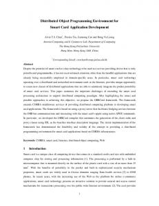
of the module. Naturally, a completely open module is one which does not hide anything from the external modules. Finally, an export declaration of a module determines a completely open basic module such that the kernel of the new module is given by the items declared for export. This determined module is designated a view module. A system specification in Troll [Har97, DH97] may be compared with a closed basic module. However, unlike Troll we do not restrict object interaction to synchronous communication, and we assume that we can express, if desired, concurrent computations explicitly. A module is either basic, as described above, or compound. A compound module consists of simpler interconnected modules. Each one of these simpler modules is again either basic or compound itself. Eventually, a compound module only contains basic modules. Moreover, a system is a compound module as well. Similarly to a basic module, a compound module has an export part. Instead of a kernel, a compound module has several parts as described next. A compound module may denote a generic (sub)system in which case some of its parts are left very general and may be replaced by more specific ones as needed. The replaceable and generic parts of a compound module build a parameter part for the module. A compound module with a parameter part is easier to reuse. Moreover, a parameterised module has a broader domain of applicability. A compound module may also contain several other modules that have been specified before. We say that these modules have been imported and build the import part of the compound module. If necessary, new classes, instances, interactions and relations may be declared in a compound module. These build the body part of the module. Recall the idea of a module as a piece of a puzzle. For a compound module such a piece is, however, a system on its own consisting of further simpler pieces. These further pieces have been imported, represent parameters, or form the module body. This idea is illustrated in Figure 2.2. An arbitrary module is considered to have five constituent parts: a parameter, an import, an export, a body and an interaction. Depending on the kind of module we have, some of these parts may be empty or not. The parameter part consists of a finite set of modules. These parameter modules are meant to be place holders, that is, modules that can be replaced by others. A module whose parameter part has at least one parameter module, is said to be generic. We assume that a parameter module is basic and corresponds to the view of another module.

2.3. Object-Oriented Modules

19

EXPORT

INTER ACTION

BODY

PARAMETER IMPORT

Figure 2.2: A compound module and its constituent parts. Import is the means by which modules may be organised into hierarchies. It denotes composition of modules. One module may import several other modules. We consider that an imported module is a view module. One can understand parameterisation as a special kind of import mechanism and vice versa. Indeed, the only notable difference is that a parameter module may be replaced, whereas an import module may not. There may be several modes to import a module. Since it is not our aim in this thesis to describe the features of an object-oriented language with modules, or MTroll in particular, we are not going to discuss the possible modes of module import. We will, nonetheless, consider that the semantics of an imported module may not be altered but only extended. The body of a module is a basic module where new object classes, objects and object interactions may be declared. A body module is completely open. Finally, all the interactions among classes or objects from the different parts of the compound module are specified in the interaction part of a compound module. The interaction part does not constitute a module on its own. According to the previous description of an arbitrary module, we understand a basic module as a module with emtpy parameter, import and interaction parts. A basic module only has a body and possibly an export part. A compound module has necessarily either a nonempty import or a nonempty parameter. A compound module may not have a body. In general a compound module should have an interaction part. A compound module

20

Chapter 2. Modules

may have an export part as well. We consider the existence of a class/module library. Such a library contains any class and module that one may wish to reuse in a certain context. Classes can only be imported into the body of a module. Modules available in the library may be imported by, or used as a parameter in, a new module. A compound module has been illustrated in Figure 2.2, and has been obtained by composing several simpler modules (imported modules, parameter modules and a body module) and adding further interactions among them. We say that the compound module belongs to a certain module level, say l, whereas its constituent modules belong to a lower level. We may now

EXPORT TO HIGHER LEVEL

MODULE LEVEL

MODULE COMPOSITION

REUSE IMPORT FROM LOWER LEVEL

Class/M odule Library

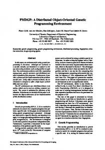
Figure 2.3: Composing modules at a certain level. take the compound module, consider one of its views determined by an export declaration, and compose it with other modules from the same level. A module in a subsequent level is obtained. This idea is illustrated in Figure 2.3. Eventually, the system level is reached. A system is a closed module. Recall the notions of framework, pattern and software architecture described in the previous section. Such notions can be found in our more abstract and general module concept as well. Indeed, frameworks, patterns

2.4. Preparing for Module Theory

21

and architectures correspond to special kinds of modules. A framework denotes a compound module with a parameter part. A pattern corresponds to a basic parameter module. Finally, software architectures may be understood as a system module, that is, a compound module importing several modules, the subsystems, and with an interaction part where the interconnections and interactions between these modules are defined. Our modules may also represent the components that in a component-based software development are plugged into a software architecture, and may be replaced whenever necessary. Comparatively to some of the programming languages mentioned, our module concept shares some of the advantages pointed out by MzScheme’s unit. The same way unit interconnections are specified outside the definitions of the involved units enhancing unit independence, module interactions are described in the interaction part of a compound module. Generic modules, import and export mechanisms resemble FOOPS constructs, even though we abstract away from some more restricted and language dependent considerations like import modes or what kind of parameter modules are allowed. As we have stated before, Java also offers a further structuring concept, namely the package construct. A package is a collection of related classes. The motivation for introducing such a concept is, however, very different than ours. Packages were introduced to avoid naming conflicts, to control class access, and to make classes easier to find and use. A class file contains a reference to the package it belongs to. Expressing dependencies internally naturally difficults reuse. By contrast, module interconnections are expressed externally in our approach. Finally, the herein given description of a module concept goes well with the MTroll approach as described in [Eck98]. It considers two structuring concepts: modules and subsystems. The difference between these concepts lies in their intended use. Whilst modules are units of reuse, subsystems constitute the building blocks for specification in-the-large. Both concepts are captured with our modules: modules correspond to our generic modules; subsystems denote (compound) modules with empty parameter part.

2.4

Preparing for Module Theory

In this section, we explain how to look at an object-oriented module from a theoretical perspective, i.e., we provide some motivation and intuition re-

22

Chapter 2. Modules

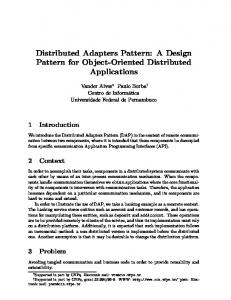
quired for understanding the module theory developed in the next chapters. As we have described before, a system may be seen as a collection of distributed and interacting object modules. A module may be more than an object and denote a parameterisable system part with intramodule concurrency. Moreover, its export declarations determine view modules that may be used for communication with other modules. An object module is either compound or basic. Semantically, we regard a basic module as a collection of concurrent and interacting objects. The objects are all the potential instances of the classes declared or available within the module. A compound module consists of simpler interacting modules. There are two ways of looking at a compound module: as a collection of interacting modules or as a collection of interacting objects. This is illustrated in Figure 2.4. A MODULE VIEWED AS A...

COLLECTION OF OBJECTS

COLLECTION OF MODULES

EXPORT

o2

o1

o3

o5

o4

BODY

o6 IMPORT PARAMETER

Figure 2.4: A twofold perspective of a compound module. In the figure, circles represent the objects, lines between circles indicate a rough representation of object interaction, and frames denote modules. A compound module has been obtained by composition of simpler modules, so it may be regarded as a collection of interacting modules (Figure 2.4 right). Within a compound module we may disregard the bounds of its constituent modules, and just consider their interface (visible) objects. Hence a compound module can also be regarded as a collection of concurrent and interacting objects (Figure 2.4 left). We assume there are no undesired name clashes of object identifiers when disregarding module bounds, that is, no


23

distinct objects are given the same identity in different modules. If an object has the same identity it corresponds to an object playing different roles in different contexts (modules). When module bounds are forgotten such objects are unified into a complex object. We will allow both perspectives on a compound module. In fact, we will use them in different situations as explained next. As we have said before, a compound module, say M , may again be part of a more complex module, say Q. If the former module M is from level k, the latter module Q belongs to a subsequent level l > k. We consider that the module M at level k is a collection of concurrent and interacting modules. The export part of module M has several export declarations defined over it. Each one of them determines a different view of M which may be imported by a more complex module. We consider that a view module is always regarded as a collection of concurrent and interacting (visible) objects instead. Consequently, the module M (one of its views) at level l is understood as a collection of concurrent and interacting objects as well. ...

MODULE LEVEL l M1 o1

M1 ⊗ M 2 ⊗ . . .

M2 o2

...

MODULE LEVEL k EXPORT N1 ⊗ N2 ⊗ N3 ⊗ N4

o2

o1 o3

o5

o4

o6

N1 ⊗ N 2 ⊗ N 3 ⊗ N 4 N2 N1

N3

N4

Figure 2.5: Moving between two immediate module levels. Figure 2.5 shows the example from Figure 2.4 at two immediate levels where l > k. At a lower level more aspects of a module are visible. This because on a higher level we just have access to a view of the module from

24

Chapter 2. Modules

the immediate lower level. At level k we have a compound module N1 ⊗N2 ⊗N3 ⊗N4 with component modules N1 . . . N4 . Each one of these modules are from a lower level than k. Except for the body module N2 , the remaining modules are view modules which have been determined by an interface of another module. The compound module exports some aspects to the upper level l. It corresponds to a view M1 of the compound module. M1 is a module at level l. At level l the module M1 may interact with other modules (M2 and so on) from the level. These again give raise to a compound module M1 ⊗ M2 ⊗ . . ., and so on. Summarising, a module belongs to a certain level (system level or below), say l, where it has been specified. At level l its constituent modules are regarded as collections of concurrent and interacting objects, whereas the compound module is understood as a collection of concurrent and interacting modules. When we reach the system level we may choose between regarding a system as a collection of objects or as a collection of modules. The same way objects have unique identifiers, we consider that each module has a unique module identifier as well. Furthermore, each module has a reference, if applicable, to the identifiers of the imported modules, the parameter modules, the body module, the view modules determined by each one of its export declarations, and its primordial module. The notion of a primordial module only makes sense for view modules. The primordial module of a view module corresponds to the module whose export part contains an export declaration that determines the view. Consider the example given in Figure 2.5, and let M be the compound module N1 ⊗N2 ⊗N3 ⊗N4 . We can say the following about module references: • M1 is a view module, and it has a reference only to its primordial module, that is, where it has been defined. The primordial module of M1 is M . • N2 is a body module. It has a reference to the module it belongs to, namely module M . • N1 and N3 are imported modules. Only views of modules may be imported, thus they have, similarly to M1 , a reference to their corresponding primordial modules. • N4 is a parameter module. Again it corresponds to a view of another (primordial) module, and has therefore a reference to it.


25

• Finally, M has a reference to all the modules N1 . . . N4 and M1 . Being compound M has a reference to its imported modules (N1 and N3 ), parameter module (N4 ), body module (N2 ), and view module (M1 ). M has no primordial module. Furthermore, the body of a basic module has the same module identifier as the basic module itself. On the other hand, if a view module corresponds exactly to its primordial module (nothing has been hidden), we will not allow them to have the same identifier. This because a view module is regarded as a collection of objects whereas a primordial module is regarded as a collection of modules. This distinction is essential for the description of a module signature as given in Section 3.2. Finally, we give some considerations on module interaction. Module interaction is done by the objects belonging to them. We permit two forms of module interactions: intermodule and intramodule interactions. The former case corresponds to interactions among objects belonging to different modules, whereas the latter case denotes internal module interactions, that is, interactions among objects belonging to the same module. Again, the form of interaction we have depend on the way modules are understood. Within a basic module we only have intramodule interactions. Intermodule interactions are specified in the interaction part of a compound module. Do notice, however, that intermodule interactions become intramodule interactions if constituent module bounds in a compound module are forgotten, and vice versa. This is also to be taken into account when changing the perspective taken on a compound module. We will come back to this point in Section 3.3.2. In any case, we allow the specification of generic and explicit interactions. A generic interaction is one where the object starting the communication calls an arbitrary instance of another class. On the other hand, an explicit interaction is one where the objects involved in the interaction are clearly indicated. Communication is considered to be synchronous or asynchronous. Synchronous communication corresponds to the simultaneous occurrence of actions of the objects involved in the communication. We present informally the conditions we impose on the asynchronous communication. We consider an asynchronous mechanism where the send of a message is non-blocking, meaning that an object can deliver a message without waiting for it to reach its destination. For asynchronous communication among

26

Chapter 2. Modules

modules what we need is a calling action from one module object, say a send action, and one or more distinct modules, where each module has one object with a corresponding called action, say a receive action. If we have only oneto-one communication we will have one calling module object with an action send and one called module with a unique object and corresponding action receive. In case of multicasting (or broadcasting) we will have one calling module object with an action send and some (or all) modules, where each has one or more objects with a corresponding action receive. In [DK96, K¨ us97c], we distinguished among communication and non-communication actions. Furthermore, a communication action may either be a send or a receive action but never both. Assumption 1 An action may be a communication or a non-communication action but not both. A communication action is either a send or a receive action but not both. We also assume in our approach that asynchronous communication is safe, i.e., for each send messages there exists a receive action in the called module(s). Assumption 2 Asynchronous communication is safe. The next assumption concerns the order of receipt of sent messages. Assumption 3 The overtaking of distinct messages is possible, i.e., the order of the occurrences of the corresponding receive actions need not be preserved. The order is considered to be preserved if the same message is sent more than once. A further assumption on asynchronous communication we take for our specification language, is that cycles are not allowed, i.e., M1 .a1 asynchronously calls M2 .a2 and so on till Mn .an asynchronously calls M1 .a1. Furthermore, by Assumption 2, an action cannot be simultaneously a send and a receive action, but a receive action can call synchronously a send action to happen. Assumption 4 The specification language does not allow calling cycles. Finally, from Assumption 1 and Assumption 4 we understand that asynchronous communication is antisymmetric. From Assumption 1 we know that we cannot express: M1 .a1 asyn calls M2 .a2 asyn calls M1 .a1

2.5. A Toy Example - Music World

27

as a1 is either a send or a receive action. On the other side, Assumption 4 makes sure that the following is not possible: M1 .s1 asyn calls M2 .r2 sync calls M2 .s2 asyn calls M1 .r1 sync calls M1 .s1

2.5

A Toy Example - Music World

We present a simple example of a Music World which we shall use throughout the thesis for illustration purposes. In this section, the example is mainly presented in natural language, however, we will often add a graphical representation to provide a better intuition and understanding. Some aspects of the example may be omitted at this point, and will be considered formally later on in the thesis. For the graphical representation we shall use an ad hoc notation in combination with some common representations of classes, associations, inheritance, and so on, as found for instance in UML. Our notation is indicated in Figure 2.6. (Class) ObjectId Object

E1 MODULE

Class Object Class

Completely Open Module E1

E2 E3 MODULE BODY

P1 P2

I1

I2

Open Compound Module

Figure 2.6: Class and Module Notations.

E2

E3

MODULE Open Module

28

Chapter 2. Modules

A completely open module is given by a double box. An open module has an indication of the export declarations it contains (e.g., E1 , E2, E3). For a compound module, we may indicate its constituent modules (all completely open): a body module (e.g., BODY), parameter modules (e.g., P1 , P2), and imported modules (e.g., I1, I2). We emphasise that the herein presented example is not meant to be complete or realistic, nonetheless it allows us to illustrate main ideas and concepts. The example covers the following aspects: module communication (synchronous and asynchronous), parameterisation and parameter actualisation, import, export and views. These aspects are formalised in subsequent chapters.

Music World: Description For our music world example, we will consider that the class/module library contains, among others, one class (Person) and two modules (CHAMBER MUSIC and DUET), to be used whenever necessary. The library is illustrated in Figure 2.7.


Person

DUET

CHAMBER MUSIC

Figure 2.7: The class/module library for Music World. Whenever a class is imported by a module, it brings with it all the potential instances of the class. This means that when an instance of a class is created in the importing module, one of its potential instances is made alive. As a consequence of this, another module importing the class may use the same instance possibly for another purpose. Even though we do not explicitly forbit this, we will not consider such a case herein.


29

Below, we describe the class and modules contained in the library. Person The attributes and actions of class Person are given in Figure 2.8. Jane, Person

(Person) Jane

name:String age:Integer profession:String ∗born(nm:String) +dead

(Person) Anna (Person) Jose

Figure 2.8: The class Person and possible instances. Jose, Anna and so on, are possible instances of the class Person. We write that Jane, Jose, Anna are elements in the set of object instances denoted by |Person|. Two actions are declared for the class: born(nm) which is used when an instance of the class is to be created (it is brought into life); dead which is used when an instance of the class is to be destroyed (it is not alive anymore). The class Person is left very general, and will be used (imported) by the modules in the system and specialised as required. CHAMBER MUSIC The module CHAMBER MUSIC is a completely open basic module. The module CHAMBER MUSIC is depicted in Figure 2.9. The module contains two classes: Chamber and Musician. The classes are linked by an association relationship: a Chamber group consists of two or more Musicians, and a Musician must belong to a group of Chamber music. We omit the actions and attributes of the classes in the graphical representation. We assume that a data type Concert has been defined as a record with the fields date:String and place:String. We consider that: • Musician has an attribute: – inChamb of type |Chamber|, reflecting the association between Musician and Chamber;

30

Chapter 2. Modules

CHAMBER MUSIC

Chamber

1 consistsOf 2..* Musician inChamb

Figure 2.9: The module CHAMBER MUSIC. and an action: – play(m:String), play a given musical composition; • Chamber has the attributes: – consistsOf of type SetOf|Musician|, reflecting the association between Chamber and Musician, – repertoire of type SetOfString, storing all the musical compositions that the group of chamber music can play, and – concerts of type SetOfConcert, storing the scheduled concerts; and the actions: – org con(c:Concert), organise a new concert, – conf(c:Concert), confirm that a concert may take place, – give con(c:Concert,m:String), give a scheduled concert playing a given musical composition, – order score(m:String), order the score for a given musical composition, – rc ordered score(m:String), receive an ordered score for a given musical composition, and – rehearse(m:String), practice a given musical composition for a public presentation. The association indicated in Figure 2.9 has been captured as attributes in both classes. In this example, birth actions for the classes have not been given for brevity. We omit the informal description of the conditions that


31

have to be fulfilled in order for an action to happen (action preconditions), and the effects of action occurrences (action postconditions). DUET DUET is a completely open basic module. It is described in Figure 2.10. The DUET Duet job:String ∗birth play(m:String)

(Duet) duet player

Constraint

job="pianist" or job="violinist"

Figure 2.10: The module DUET. module is left as simple as possible and contains a class Duet. The class has an attribute job and actions birth and play(m). Additionally, a constraint on the possible values of the attribute job is given. An instance duet player of the class Duet is declared. Moreover, as a consequence of the stated constraint, a valid instance of Duet is either a pianist or a violinist and nothing else. The music world example consists basically of the two modules indicated in Figure 2.11, namely MUSIC SCHOOL and CELLIST[DUET]. These modules will enable us to illustrate some module concepts and constructions throughout the thesis. We will start giving a rough description of the module MUSIC SCHOOL. MUSIC SCHOOL Figure 2.12 presents some static aspects of the module MUSIC SCHOOL. The module MUSIC SCHOOL may be described as follows:

32

Chapter 2. Modules


CELLIST[DUET]

MUSIC SCHOOL

Figure 2.11: The components of Music World. • MUSIC SCHOOL is a compound module with import, body, export (not indicated in Figure 2.12) and interaction parts. The import part consists of one module, module C which corresponds to a renaming of CHAMBER MUSIC. The body module BODY imports the class Person from the library. We describe the interaction and export parts separately. • The class Person is specialised into the classes Teacher and Student. • The class Student is further specialised into the classes Cello Std, Piano Std and so on. Also the class Teacher is further specialised into the classes Cellist, Pianist and so on. • A Teacher may be responsible for a certain number of ChamberM groups. Conversely, a ChamberM group has one responsible Teacher. The association is captured by corresponding attributes in both classes. • The class Student has an attribute member of a data type choice, an enumerated type enum(orchestra,chorus,chambermusic): each Student may either be a member of the orchestra, sing in the schools chorus or alternatively play chambermusic. A further attribute of class Student is year. One action of the class is play(m): play a given musical composition. The following constraint is considered: – to be allowed to be a member of chambermusic a student has to be in the 3rd or higher year;


33

MUSIC SCHOOL BODY Person

Cellist

Teacher

Pianist

Student

...

Cello Std

...

1

Piano Std memberOf

1

Secretary

C 0..1

responsibleFor

1

ChamberM in

group 2..*

CMStudent

0..*

Figure 2.12: The module MUSIC SCHOOL. • A Student that is a member of chambermusic is a CMStudent. A CMStudent is a Student. • The class Secretary takes care of all the administrative work of the school. We will see that this class is involved in the intermodule interactions with module C. The class has two attributes: – toDoConcerts of type SetOfDoCon, reflecting the set of concerts with pending arrangements. The data type DoCon is considered a record with fields con:Concert and who:|Object|, – toDoOrders of type SetOfDoOrd, reflecting the set of scores of musical compositions that have not yet been ordered. The data type DoOrd is considered a record with fields piece:String and who:|Object|, and the following actions

34

Chapter 2. Modules – organise(x:DoCon), organise a concert x.con for the chamber music group x.who, – call(x:DoCon,!b:bool), settle the arrangements for a concert x.con and find out it if is possible or not. The boolean output parameter b will store the result accordingly, – confirm(x), confirm to the group x.who that the arrangements for the concert x.con are settled, – rc order(o), receive an order for a score of a musical composition o.piece from o.who, – order(o), work out a request for the score of a musical composition o.piece from o.who ordering it as appropriate, – receive(o), receive an order o for a request that has been worked out previously, – deliver(o), deliver the score of a musical composition o.piece to o.who. • We assume that the following instances of the classes have been declared and are alive at a certain point in time: Anna is a Pianist, Jose is a Cellist, Jane is a Cello Std, Mary is a Piano Std, Laura and Bob are instances of class Secretary, and Cmg is an instance of class ChamberM. Moreover, Jane and Mary are CMStudent.

We now describe the synchronous and asynchronous interactions between the components of the module MUSIC SCHOOL. Synchronous Interactions between C and BODY: At the end of a term a group of chamber music might feel prepared to give a concert. The Secretary is contacted and asked to take care of the organisational details of the concert. I.e., the action org con(c) for ChamberM calls the action organise(x) of Secretary, whereby x.con is c and x.who is the group’s identifier with type |ChamberM| ⊆ |Object|. The communication between ChamberM and Secretary is synchronous. The Secretary takes a note on the planned concert. Eventually, the Secretary gives a call in order to settle the arrangements and find out if the concert is possible on such a date and place. It corresponds to the action call(x,b), whereby b is an output boolean parameter which takes the value


35

true if the concert may take place and false if not. Later on, if the concert may take place on x.con.date and at x.con.place as desired, the group of chamber music receives a confirmation. Again, this denotes a synchronous communication between Secretary and ChamberM. Asynchronous Interactions between C and BODY: A group of chamber music has a repertoire, storing all the music pieces that the group can play. A group may wish, though, to extend its repertoire of musical compositions, and in such a case it has to acquire the score of a new musical composition. It sends a request to the Secretary to order the score of a given musical composition. I.e., the action order score(m) for ChamberM calls asynchronously the action rc order(o) of Secretary, whereby o.piece is m and o.who is the identifier of the instance of class ChamberM starting the asynchronous communication. The Secretary receiving the request is responsible for carrying out the order. Eventually, the Secretary will receive an ordered book and will be able to deliver it further to the corresponding group of chamber music. A new asynchronous communication between Secretary and ChamberM starts. Export Part of MUSIC SCHOOL: We consider that the module has five export declarations (E1 , . . . , E5) determining consequently five views of the module MUSIC SCHOOL. The view modules (V1, . . . , V5 ) will be described in detail in the next chapter. We therefore postpone their presentation till then. CELLIST[DUET] For this module, consider that the module V4 is a view of MUSIC SCHOOL hiding everything except the class Cellist. An instance Jose has been declared for class Cellist. The module CELLIST[DUET] imports the view V4 of MUSIC SCHOOL and has as a parameter the module DUET from the library. Figure 2.13 illustrates the module CELLIST[DUET]. Some details of the module DUET have been omitted. A complete description of the module DUET has been given in Figure 2.10. Let another view of MUSIC SCHOOL be the module V5 hiding everything except the class Pianist. Anna is an instance of class Pianist. The module

36

Chapter 2. Modules

CELLIST[DUET]

DUET Duet play(m)

V4 Cellist favourites play solo(m) play duet(m)

Figure 2.13: The module CELLIST[DUET]. DUET can be instantiated by V5 in CELLIST[DUET] whereby we obtain the module CELLIST[V5].

2.6

Summary

In this chapter, we have seen the evolution of modularisation concepts from simple routines in the 1950s to more complex objects, frameworks and components in the current days. We have discussed recent, not yet standardised, concepts like frameworks, patterns, components and software architectures as seemed more appropriate to us. In this context, we have delineated the object-oriented module concept that we shall adopt in this thesis. At a high level of abstraction on the one side, and from a theoretical and languageindependent perspective on the other, it is not necessary to distinguish among most of these concepts. Our module concept integrates frameworks, patterns, and architectures in a single unit. Indeed, frameworks, patterns and architectures correspond to special kinds of modules. A framework denotes a compound module with a parameter part. A pattern corresponds to a basic parameter module. Finally, software architectures may be understood as a compound module importing several modules, the subsystems, and with an interaction part where the interconnections and interactions between these modules are defined. For the theory developed in the subsequent chapters it is important to understand how to regard a module. A twofold view on a

2.6. Summary

37

module may be adopted: a module may be seen as a collection of concurrent interacting modules, or as a collection of concurrent interacting objects. Finally, a toy example Music World has been given, and will be used throughout the thesis for illustrating the object-oriented module semantics.

39

Chapter 3 Module Specification A module concept for object-oriented languages has been proposed in the previous chapter. In this chapter, we put forward its formalisation. We use a logical framework for the formalisation of object-oriented languages with modules, i.e., we consider module descriptions to be theory presentations of a certain logic. A module description is a pair consisting of a module signature, defining the specific vocabulary symbols that are relevant for the description of the module, and a set of module axioms, a collection of formulae in the logic generated from the signature. A module description is often called module specification. In this chapter, we define the notion of a module signature and describe the module logic we shall adopt. The logic that has been developed for describing modules is called Mdtl which stands for Module distributed temporal logic. Mdtl is interpreted over labelled prime event structures. The chosen interpretation structures are subject of Chapter 4, and we therefore postpone the presentation of the semantics of Mdtl to Section 4.3. In this chapter, we start giving a brief description of several approaches and directions found in the literature in order to formalise object-oriented concepts. Recent foundational work around the Troll language is explained with more care, as it forms the basis of our approach to object-oriented modules. In Section 3.2, several concepts are introduced in order to be able to define a module signature. It is followed by Section 3.3, where the syntax of the module logic Mdtl is given. Section 3.4 gives the formal definition of a module specification as a theory presentation of Mdtl. Finally, Mdtl and some particular logics are compared in Section 3.5. Attention is given to logics for concurrency and distribution, logics supporting modularisation

40

Chapter 3. Module Specification

as used in modular logic programming, and object logics.

3.1

Object Specification

In the next subsection, we start with a brief survey of distinct approaches that have been developed through the years to provide a well-defined semantic foundation to object-oriented languages. We will concentrate our attention specially on the approaches that are more closely related to the Troll foundations. Other similar foundations of object-oriented approaches with module concepts found in the literature are outlined. The starting point of the module theory developed in this thesis is discussed in Subsection 3.1.2.

3.1.1

Survey of Object Foundations

Ever since object-oriented languages have become popular in the field of software engineering, researchers started working on their theoretical foundations. Many different directions have been proposed and followed for this purpose using: type-theory, the actor model, process calculi, Petri nets, finite state machines, algebraic specification, a logical framework, or else. Each of them has its own specific merits, and we describe briefly some of them below. A lot of effort has been put into using type-theory to provide a foundation for programming languages in general [Gun92, Mit96], and for object-oriented programming languages in particular. Most of the type-theoretic approaches developed for object semantics have a common root in typed λ-calculus. Among them we have the work reported in [CW85, GM94b, AC96, PT94, Mit96, FM97, Red98], to cite just a few. In a type-theoretic approach, an object is viewed as a record of functions together with a hidden representative type. One advantage of using typed λ-calculus is that it deals well with some object-oriented features like object encapsulation and identity, message passing, subtyping and polymorphism. However, it deals with state change either in a roundabout way or not at all. Furthermore, typed λ-calculi are useful for studying the axiomatic, operational, and denotational semantics of sequential programming languages, whereas they are not adequate for dealing with concurrent programming languages. Perhaps one of the first approaches dealing with concurrency in distributed object systems was the actor model [Agh86, Agh90]. The actor model concentrates on the behaviour of objects/actors. The behaviour of objects is

3.1. Object Specification

41

understood as functions of incoming computations. Actors were introduced by Carl Hewitt at the MIT in the early 1970s to describe the concept of reasoning agents. Actors are self-contained, interactive, independent components of a computing system that communicate by asynchronous message passing. An actor can create other actors, send messages, and modify its own local state. Actors can have an effect on the local state of other actors by sending them messages. In the actor model, concurrent computations are represented by event diagrams, which have been developed to model the behaviour of actor systems. These diagrams use lifelines to represent the sequential behaviour of actors. Actor creations, message passing, event causality and event pending can be represented in such diagrams. The event diagrams can be given a semantics in terms of power domains. Over the years some concurrent object-oriented languages have been defined in accordance to the actor model. Such languages are often called actor languages instead of object-oriented. Actor languages have been treated semantically in, e.g., [AMST92, Agh91, MT99, VT92]. An alternative direction uses process calculi to provide an operational semantics for object-oriented languages. An object is now regarded as a process, whereby the current state of an object is given by its current behaviour. Among the process calculi found in the literature, the π-calculus is probably the most well-known “mobile” process calculus supporting concurrency [MPW92]. Moreover, the π-calculus is considered to analyse and clarify the world of concurrently communicating processes in much the same way as λ-calculus and other models of computation have done for the sequential world. Many approaches based on the π-calculus have been developed for dealing with concurrent object-oriented languages. Examples include the Object Calculus [Nie92], which is basically a unification of the π and λ calculi in order to handle concurrent objects; and the calculus presented in [HT92], which is based on a fragment of the π-calculus and focuses on asynchronous communication. Also several extensions of CCS are used to describe the behaviour of objects, e.g., in [Pap92] a CCS-based framework for defining the semantics of concurrent object-based languages is proposed. The framework supports object-oriented features like encapsulation, object identity, classes, inheritance and concurrency. Furthermore, [Smo97] describes a computational calculus for higher-order concurrent programming, namely the γ-calculus, which may also be used for expressing concurrent objects with encapsulated state and multiple inheritance. Algebraic specification was introduced in the 1970s for the mathematical

42


foundation of abstract data types and the formal development of applicative programs. Nowadays, algebraic specification is used in many more applications including the uniform definition of syntax and semantics of programming languages [AKKB99]. However, in order to handle properly concurrent and reactive systems, it is necessary to extend the algebraic techniques in some way [ABR99]. An example is given with [BZ96], where algebraic specification has been used to formalise concurrent object-oriented languages. For modelling the dynamic behaviour of objects an algebraic description of labelled transition systems is used. Both ideas from algebraic specification and process theory have been combined to obtain a model for object-oriented concepts in several papers [EGS92, ESS88, ESS89, ESS90, ES91, SEC90, SFSE89, SSE87, SE91]. Such theoretical achievements led to the development of a family of high-level system specification languages and design methodologies that started with Oblog [SSG+ 91, SGCS91] and evolved in Troll [JSHS91, HSJ+ 94, DH97] and Gnome [SR94]. In the foundational work of such languages, an object is viewed as a sequential process endowed with trace-dependent attributes (cf. e.g. [SEC90, SE91]). A notion of process morphism is introduced yielding a category of processes. In such a framework, categorical constructions allow the description of several concepts like object interaction, reification, encapsulation, inheritance and aggregation (cf. e.g., [ES91]). Apart from the work on semantic models, also logical fundamentals for object specification started being envisaged. In a logical approach to object specification, object and system properties are expressed as formulae in a logic. Moreover, an advantage of using temporal logic consists in the ability to express liveness, fairness and safety constraints of reactive systems [Pnu77]. Work on linear temporal logics for object specification in the previous setting includes [FM92, SSC95, SSR96, EJDS94]. In a logical framework, an object is specified as a theory presentation of a temporal logic, whereby a theory presentation consists of a signature and a set of axioms in the logic. The signature describes the structure of the object whereas the axioms describe its behaviour. Categorical constructions allow the composition of object theories to describe systems of interconnected objects [FM92]. Moreover, the advantages of institutions [GB92] as an abstract model independent of an underlying logic started being recognised and used for establishing a categorical, denotational semantics of several basic constructs of object specification, including aggregation, interconnection, abstraction and monotonic

3.1. Object Specification

43

specialisation [SSC98]. In order to cope with concurrency, a new semantic model is considered in subsequent work. Instead of traces or life cycles, which are sequential models, a true-concurrency model is adopted, namely labelled prime event structures or event structures for short. The behaviour of an object is modelled by a sequential event structure. How to define concurrent composition of object models for event structures is described in [ES95] using an inductive construction. The system model consists of the models of its objects glued together at shared events. Shared events reflect synchronous communication among the objects. Further object-oriented concepts and constructions like refinement, inheritance, several forms of composition, and interaction are described in [Den96b, EH96, Ehr99]. A linear temporal logic for object specification interpreted over event structures is given in [ESSS94, ES95, EH96, Ehr99]. More recently, inspired by n-agent logics like [LRT92], object locality is introduced in object logic and a so-called distributed temporal logic dtl is developed [DE97, ECSD98, EC00]. A system is now described from the local viewpoint of its component objects. An object has a local logic for expressing internal properties (home logic), and to describe knowledge it has acquired from others through communication (communication logic). Some object-oriented languages that make a distinction between modules and objects or classes, as discussed in the previous chapter have a well-defined semantics. Foops [GM87] is based on algebraic techniques, namely hiddensorted equational logic and sheaf theory [WG92]. Similarly, Maude is also based on algebraic techniques but relies on an operational semantics based on rewriting logic [Mes92]. Order-sorted algebra has been described in [GM92] and supports objectoriented concepts like multiple inheritance, several forms of polymorphism and overloading, partial operations and exception handling. Hidden-sorted algebras additionally cover object encapsulation. However, dynamic aspects are not addressed in such an algebraic framework. Within the algebraic setting, several module constructions have been defined including module composition, parameterisation and refinement [EM90, EMCO92, EMO92, EGR94, EHKPP91, LEW96]. However, our approach to object-oriented modules is somehow different in that we are based on a different source of work, namely on work developed around object foundations. More recently, object-oriented design (OOD) frameworks have received much attention in component-based software development. OOD frameworks are collections of (interacting) objects, and important units of reuse in

44


software development. OOD frameworks correspond to a particular kind of object-oriented modules as adopted in this thesis as described in the previous chapter. OOD frameworks have not received much attention in theory and there is no adequate formalisation available. Work on their formalisation has been carried out by Lau and Ornaghi in [KLO96, LO99, LO98] among others. However, their approach only defines a static semantics for OOD frameworks based on first-order theories with isoinitial models. Dynamic issues like state transitions and framework interactions have not been considered. Dynamic aspects are a fundamental feature of object-orientation in general and objectoriented frameworks in particular. Such issues must be fully addressed in an adequate formalisation.

3.1.2

Module Specification: Preliminaries

A starting point for the theoretical foundations of object-oriented modules is the work done on object specification, specially the one developed more recently around the Troll language [ES95, Ehr99, DE97, ECSD98], and related approaches like [FM92, SSC95]. However, also other approaches from outside the object-oriented world that consider module concepts, like algebraic specifications [GM92, EM90, LEW96], modular logic programming [BLM94, BGM98, BMPT94, GM94a, Mil89], among others, have been influential. An object, class or system has a structural and a behavioural part. The structure of an object, class or system is described algebraically by a so-called extended data signature [ES95]. An extended data signature Σ is interpreted over Σ-algebras. A notion of morphism between Σ-algebras exists, and thus also a category of Σ-algebras. The behaviour is described as a set of formulae in dtl (Distributed temporal logic), or D0 as it is referred to in some papers [DE97, ECSD98]. dtl is a linear discrete distributed propositional temporal logic. The idea of the logic has been described before and consists of object locality, i.e., each object in a system has a local logic allowing it to make assertions about itself and system properties from its local viewpoint. The logic is interpreted over labelled event structures. The behaviour of an object is modelled by a sequential labelled event structure. A system model is obtained by concurrent composition of object models. As mentioned before, [ES95] defines an inductive construction for concurrent composition. In order to formalise object-oriented modules, we need to extend the

3.2. Module Signature

45

structural description of objects and systems to cover our notions of basic and compound modules. Furthermore, we need to extend dtl in such a way that it allows us to reason about modules as the main unit instead of the objects. The object locality of dtl should thus be shifted to a module locality in Mdtl. Modules are more complex than objects, and represent a collection of interacting objects. A module may contain internal concurrency and internal communication, and may consist of several simpler (imported or parameter) modules. Modules may communicate synchronously or asynchronously with one another. We thus have to be able to deal with various new aspects, namely module encapsulation (abstraction), internal module concurrency, module composition, communication, parameterisation and refinement. In the next section, we define a notion of module signature to capture the structural aspects of our object-oriented modules. Class signatures are recalled and gradually enriched to describe modules. In Section 3.3, we define a module logic Mdtl that extends dtl and covers new aspects of modules like concurrency and several communication facilities. Mdtl contains a concurrency operator in the style of the n-agent logic described in [Chr90]. Module specifications are theory presentations of Mdtl consisting of a pair of a module signature and a set of Mdtl formulae, the axioms of the module. Finally, we need to define new semantic constructions for modules, namely synchronous and asynchronous concurrent composition, encapsulation (abstraction), renaming, parameter actualisation and refinement. These constructions are subject of Chapter 5.

3.2

Module Signature

In Chapter 2, we described the object-oriented module concept adopted in this thesis. In this section, we start formalising object-oriented modules by introducing the notion of a module signature. As we have mentioned before, a module can either be basic or compound. This distinction is naturally reflected in the definition of a module signature. We present the definition of a module signature gradually. We start recalling the definition of a class signature in the next subsection. This definition is extended to a basic module signature in Subsection 3.2.2 and a module signature in Subsection 3.2.3.

46


3.2.1

Class Signature

A basic module consists of a group of related and interacting classes/objects. The simplest form of a (basic) module is thus a single class. Therefore, before we introduce the notion of a module signature we present the definition of a class signature. The herein used definition of a class signature is a slightly modified version of the one introduced by Ehrich and Sernadas in [ES95]. We consider order-sorted signatures instead of just many-sorted signatures as is done in [ES95]. Order-sorted signatures have also been considered in [Den96b]. Our presentation of class signatures still differs from [Den96b] in some ways. Essentially, we explicitly deal with attributes which is not done in [ES95, Den96b, Har97]. First of all we recall the definition of an order-sorted data signature as given in [GM92]. Definition 3.1 (Order-Sorted Data Signature) An order-sorted data signature is a triple ΣD = (SD , ΩD , ≤D ) where: • SD is a finite set of data sorts; ∗ × SD -indexed family of sets of data operations, and • ΩD is an SD

• ≤D ⊆ SD × SD is a binary relation on the set of data sorts such that (SD , ≤D ) is a partial order (reflexive, antisymmetric and transitive). The following monotonicity condition is satisfied: if o ∈ ΩD s1 ...sn ,s ∩ ΩD r1 ...rn ,r and si ≤D ri for 1 ≤ i ≤ n then s ≤D r Let dat be the maximal data sort, i.e., for any data sort s ∈ SD we have s ≤D dat. For each o ∈ ΩDw,s , w is the parameter list of the operation o and s the result sort. The elements of ΩD ε,s are called constant symbols of sort s, or just constants for short. We may write o : w → s or o : s1 × . . . × sn → s for o ∈ ΩDw,s with w = s1 . . . sn , and o :→ s for o ∈ ΩDε,s . The partial order on 0 the data sorts specifies a subsort relation, i.e., if s ≤D s then we say that s 0 0 is a subsort of s , or equivalently s is a supersort of s. The monotonicity condition on the operations allows one to deal with partial functions, overloading and polymorphism. It is particularly important


47

for expressing inheritance and polymorphism in object-oriented languages. We refer the interested reader to [GM92] for a detailed presentation of ordersorted signatures, algebras, and categorical results. Examples of data sorts are bool, the ordered sorts nat ≤D int ≤D real, string, dat, and so on. We also may consider more complex sorts like parameterised data sorts (e.g., list(dat), set(dat), stack(dat)), records, and so on. Examples of data operations include string concatenation conc; data operations on the booleans like true, f alse, not; the overloaded operation isIn checking if an element of sort dat is in a set of elements of the same sort, and so on. Since isIn is overloaded, we may have isIn ∈ ΩD string set(string),bool and thus use it for checking if a string is in a set(string). How to deal semantically with complex data sorts is assumed understood. More details can be found in several work in the literature focusing on abstract data types, e.g., [LEW96, EGL89]. Morphisms between order-sorted (data) signatures may be defined. Ordersorted (data) signatures and morphisms form a category. We omit the notion of an order-sorted (data) signature morphism for the moment. Let X be an SD -indexed family of disjoint sets of variables. A data signature may be extended with variables by considering them as constant symbols of a given sort. A data signature with variables is sometimes written ΣD (X). From the symbols defined in the order-sorted data signature and the variables it is possible to construct data terms. Definition 3.2 (Data Terms) Let ΣD = (SD , ΩD , ≤D ) be an order-sorted data signature and X be an SD -indexed family of disjoint sets of variables. The family of data terms over ΣD and X, TΣD (X), is an SD -indexed family of disjoint sets defined inductively as follows: • If o ∈ ΩD ε,s then o ∈ TΣD ,s (X); • If x ∈ Xs then x ∈ TΣD ,s (X); • If o ∈ ΩDw,s , w = s1 . . . sn 6= ε, ti ∈ TΣD ,si (X) for 1 ≤ i ≤ n, then o(t1 , . . . , tn ) ∈ TΣD ,s (X). 0

• If s ≤D s then TΣD ,s (X) ⊆ TΣD ,s0 (X) Constants and variables denote basic terms. Other terms can be obtained by recursively applying the operations on terms, starting with the

48


basic terms. Furthermore, terms of a given sort s are also terms of a super0 sort s . The elements of TΣD ,s (X) are called data terms of sort s over ΣD (X). The family TΣD (∅) is the family of closed terms, also written TΣD . The interpretation structure over an order-sorted data signature ΣD is an order-sorted ΣD -algebra. Consider the following definition of an order-sorted Σ-algebra defined over an arbitrary order-sorted (data or else) signature Σ. Definition 3.3 (Order-Sorted Σ-Algebra) Let Σ = (S, Ω, ≤) be an ordersorted signature. An order-sorted Σ-Algebra AΣ is a pair (A,O) where: • A is an S-indexed family of sets (carrier sets), i.e., A = {As}s∈S . • O is an S ∗ × S-indexed family of mappings, such that: – Oε,s : Ωε,s −→ As ; – Os1 ...sn ,s : Ωs1 ...sn ,s −→ [As1 × . . . × Asn → As ]. The following monotonicity conditions are satisfied: 1. if s1 ≤ s2 in S then As1 ⊆ As2 ; and 2. if o ∈ Ωs1 ...sn ,s ∩ Ωr1 ...rn ,r and si ≤ ri for 1 ≤ i ≤ n then O(o)(u1 , . . . , un ) = O(o)(q1 , . . . , qn) with ui ∈ Asi and qi ∈ Ari . For each sort s ∈ S there is a corresponding carrier set As . To each constant o of sort s an element of the carrier set As is associated, i.e., O(o) = a with a ∈ As . The interpretation of an operation o : s1 ×. . .×sn → s is given by O(o) = oO : As1 ×. . .×Asn → As . The partial order on the sorts is reflected as an inclusion on the corresponding carrier sets. Furthermore, the second monotonicity condition states that there is an interpretation agreement on the domain intersection of overloading operations. Terms denote a certain value, so it must be possible to evaluate a term under a given interpretation. Definition 3.4 (Assignment and Data Term Interpretation) Let ΣD be an order-sorted data signature ΣD = (SD , ΩD , ≤D ), X be an S-indexed family of disjoint sets of variables, and AΣD be a ΣD -Algebra AΣD = (A, O). A variable assignment over X in AΣD is an SD -indexed family of mappings, ρ : X → A. To each variable x ∈ Xs a value in the carrier set As is associated. A term interpretation in AΣD for an assignment ρ over X, is an SD -indexed family of mappings Iρ : TΣD (X) → AΣD defined as follows:


49

• Iρ,s (o) = Oε,s (o), where o ∈ ΩD ε,s ; • Iρ,s (x) = ρs (x), where x ∈ Xs ; • Iρ,s (o(t1 , . . . , tn )) = Os1 ...sn ,s (o)(Iρ,s1 (t1), . . . , Iρ,sn (tn )), where ti ∈ TΣD ,si (X) for 1 ≤ i ≤ n. We may omit the index ρ for closed term interpretation. We want to extend order-sorted data signatures in such a way that they describe classes, and their interpretations are still given by order-sorted Σalgebras as defined above. For describing a class signature, apart from data sorts and operations, we will need object sorts (SO ) and operations on them (ΩO ). Intuitively, each class is equipped with such an object sort. Since classes can be arranged in hierarchies through inheritance, a partial order defined on the object sorts reflects such an inheritance relation. A class describes the attributes and actions of its potential instances. Attributes, actions, and instances can be understood as special object operations. Consider the following preliminary notion of a class signature. Definition 3.5 (Class Signature) A class signature over an order-sorted data signature ΣD is given by CΣD = (SO , ≤O , I, AT, AC). Let S = SD ∪ SO . CΣD is such that: • SO is a finite set of object sorts, • ≤O ⊆ SO × SO is a binary relation on the set of object sorts such that (SO , ≤O ) is a partial order; • I is an S ∗ × SO -indexed family of sets of instance operations; • AT is an SO × S-indexed family of sets of attribute operations; • AC is an S ∗ × SO -indexed family of sets of action operations. Let obj be the maximal object sort, i.e., for any object sort s ∈ SO we have s ≤O obj. The set of sorts SO contains the object sort associated to the class, as well as the sorts of the other related classes (e.g., superclasses). We assume that there is a class Object with sort obj that is the superclass of all classes.

50


The binary relation ≤O on object sorts denotes the inheritance relation. If two object sorts s1 and s2 are ordered, that is s1 ≤O s2, then we say that the class with object sort s1 inherits from the class with sort s2. In other words, the class with object sort s1 is a subclass of the one with object sort s2 . Conversely, the class with object sort s2 is a superclass of the one with object sort s1. Since the class Object with sort obj is the superclass of all classes, we have s ≤O obj for any sort s ∈ SO . Attribute, action and instance operations as defined above carry with them some reference to the object sort they correspond to. For an instance operator i ∈ Ix,s , x is the (possibly empty) parameter list of i and s denotes its object sort. Similarly, for an action operator a ∈ ACx,s , x is the (possibly empty) parameter list of a and s denotes its object sort. For an attribute operator o ∈ ATs1,s2 , s1 is the underlying object sort of the attribute and s2 is its result sort. The fact that instances, attributes and actions have a reference to their underlying object sort, and thus a reference to the class they correspond to, makes the definition of a class signature as given above very general. Consequently, such a signature definition is not only applicable to single classes, or even classes related by inheritance, and may be used to describe entire collections of classes. Indeed, the above given definition of a class signature may be used to describe the signature of a system as understood in Troll. We will come back to this in the next subsection when treating basic modules. Example 3.2.1 Consider the class Person from the Music World example as described on page 29. Let the data signature contain the data sorts string and integer. The class signature of Person is given by: PersonΣD = (SO , ≤O , I, AT, AC) with SO = {person, obj} ≤O = {(person, obj)} ∪ {(s, s) | s ∈ SO } Iε,person = {Anna, Jose, Jane, Mary} ATperson,string = {name, profession} ATperson,integer = {age} ACε,person = {dead} ACstring,person = {born}

In the above signature, the constants Anna, Jose, Jane and Mary are instances of the class. The attributes name and profession have result type


51

string, whereas age has the result type integer. The action dead has no arguments, whereas the action born has one parameter of sort string. Consider the class Student as described in the module MUSIC SCHOOL. The class Student is a subclass of Person. We thus have the following class signature for Student: StudentSΣD = (SO , ≤O , I, AT, AC) with SO = {person, student, obj} ≤O = {(student, person), (student, obj), (person, obj)} ∪ {(s, s) | s ∈ SO } Iε,student = {Jane, Mary} Inat,student = {s} ATstudent,choice = {member} ATstudent,nat = {year} ATstudent,string = {name, profession} ATstudent,integer = {age} ACstring,student = {born, play} ACε,student = {dead}

Since Student inherits from Person, it inherits all the attributes and the actions declared for Person. 2 It does not suffice to distinguish among data and object sorts and operations, if we want to shorten the above definition of a class in such a way that it extends the notion of an order-sorted data signature. That is, we want to redefine a class signature as a triple consisting of (data and object) sorts; (data and object) operations; and a partial order among sorts. Object operations include the special operations like instance, attribute and action operations. However, we need to know whether a certain object operation is an action operation or else. Thus, we need to distinguish between: an attribute object sort (SOat), an action object sort (SOac ), and an instance object sort (SOi ). We introduce the concept of an extended order-sorted signature as follows. Definition 3.6 (Extended Order-Sorted Signature) Let CΣD be a class signature defined over an order-sorted data signature ΣD . An extended order-sorted signature determined by CΣD consists of a triple Σ = (S, Ω, ≤), defined as follows:

52

Chapter 3. Module Specification • S is a finite set of sorts, data and object sorts, that is, S = SD ∪ SO whereby SO = SOi ∪ SOat ∪ SOac is a union of disjoint sets such that for any object sort s from CΣD we have si ∈ SOi , sat ∈ SOat and sac ∈ SOac . • Ω is an S ∗ × S-indexed family of sets of operation symbols such that ΩD ⊆ Ω. Let S i = SOi ∪ SD . Further operations in Ω are the instance, attribute and action operations available in CΣD which correspond to the following special operations: ∗

– Ωsi xi ,si with xi ∈ S i and si ∈ SOi corresponds to the instance operations of CΣD given by Ix,s; – Ωsi sat ,ri with si ∈ SOi , sat ∈ SOat and ri ∈ S i corresponds to the attribute operations of CΣD given by ATs,r ; and ∗

– Ωsi xi ,sac with si ∈ SOi , x ∈ S i and sac ∈ SOac corresponds to the action operations of CΣD given by ACx,s. No further operations are available in Ω. • ≤⊆ S × S is a binary relation on the set of sorts such that (S, ≤) is a partial order. ≤ is such that its restriction to the data sorts corresponds to ≤D . Moreover, for any two object sorts from CΣD such that s1 ≤O s2, i ac ac at we have si1 ≤ si2 , sat 1 ≤ s2 , and s1 ≤ s2 . We write id = obj , at = obj at and ac = obj ac . The following monotonicity condition is satisfied: if o ∈ Ωs1 ...sn ,s ∩ Ωr1 ...rn ,r and sj ≤ rj for 1 ≤ j ≤ n then s ≤ r In the above definition, attributes and actions contain as an argument a reference to the object instance they are referring to. For example, for an attribute operation o ∈ Ωsi sat ,ri the reference to the instance it corresponds to is given by si . Furthermore, the duplication of the instance sort in an instance operation o ∈ Ωsi xi ,si is necessary to allow instance operations to be inherited by subclasses. Otherwise, the monotonicity condition would never be satisfied for instance operations. Some of our examples may also contain parameterised instance object sorts like set(s) where s ∈ SOi . Such complex sorts can be dealt with in very much the same way as done with parameterised data sorts. We will not go into further details.


53

Example 3.2.2 The extended order-sorted signature determined by the class signature StudentΣD from Example 3.2.1 is given by: Σstudent = (S, Ω, ≤) with S = S D ∪ SO SD = {choice, string, integer} SO = {studenti , studentat , studentac , id, at, ac} Ω: ΩD (omitted) Ωstudenti ,studenti = {Jane, Mary} Ωstudenti nat,studenti = {s} Ωstudenti studentat ,string = {name, profession} Ωstudenti studentat ,integer = {age} Ωstudenti studentat ,choice = {member} Ωstudenti studentat ,nat = {year} Ωstudenti ,studentac = {dead} Ωstudenti string,studentac = {born, play} ≤= {(studenti , id), (studentat, at), (studentac , ac)} ∪ {(s, s) | s ∈ S}

2 The following definition describes the notion of a morphism between extended order-sorted signatures. Morphisms between signatures allow us to relate different signatures. In particular, they are important for renaming, parameterisation and refinement. We will come back to such considerations later on in this thesis. Definition 3.7 (Extended Order-Sorted Signature Morphism) Let Σ1 and Σ2 be extended order-sorted signatures, Σ1 = (S1 , Ω1 , ≤1) and Σ2 = (S2 , Ω2 , ≤2). An extended order-sorted signature morphism σ : Σ1 → Σ2 is a pair of maps σ = (σso , σop ) such that • σso : S1 → S2 is an order preserving map between sorts, i.e., if s ≤1 s 0 then σso (s) ≤2 σso (s ), and

0

• σop : Ω1 → Ω2 is an S1∗ × S1 -indexed family of mappings σop = {σop s1 ...sn ,s : Ω1 s1 ...sn ,s → Ω2 σso (s1 )...σso (sn ),σso(s) }s1 ...sn ∈S1∗ ,s∈S1 From an extended order-sorted signature we can construct not only data terms (as in Definition 3.2) but instance, attribute and action terms. For a

54


given signature Σ(X), we will denote TΣ (X) the family of sets of data and instance terms, AT TΣ(X) the family of sets of attribute terms, and ACTΣ(X) the family of sets of action terms. Definition 3.8 (Terms) Let Σ be an extended order-sorted signature Σ = (S, Ω, ≤), and X be an S i -indexed family of sets of variables. TΣ (X) is an S i -indexed family of sets of data and instance terms inductively built as follows: 1. If o ∈ Ωε,s then o ∈ TΣ,s (X); 2. If x ∈ Xs then x ∈ TΣ,s (X); 3. If o ∈ Ωw,s , w = s1 . . . sn 6= ε, s1 6= s 6∈ SOi , sj , s ∈ S i , tj ∈ TΣ,sj (X) for 1 ≤ j ≤ n, then o(t1 , . . . , tn ) ∈ TΣ,s (X), 4. If o ∈ Ωs,s , s ∈ SOi then o ∈ TΣ,s (X) 5. If o ∈ Ωw,s , w = s s1 . . . sn 6= ε, s ∈ SOi , tj ∈ TΣ,sj (X) for 1 ≤ j ≤ n, then o(t1 , . . . , tn ) ∈ TΣ,s (X). 0

6. If s ≤ s , then TΣ,s (X) ⊆ TΣ,s0 (X). AT TΣ(X) is an S i -indexed family of sets of attribute terms built as follows: 1. If a ∈ Ωsi sat ,r , si ∈ SOi , sat ∈ SOat, and t ∈ TΣ,si (X) then t.a ∈ AT TΣ,r (X). 2. If r ≤ q, then AT TΣ,r (X) ⊆ AT TΣ,q (X) ACTΣ(X) is an SOac -indexed family of sets of action terms built as follows: 1. If c ∈ Ωsi ε,sac , si ∈ SOi , sac ∈ SOac , and t ∈ TΣ,si (X) then t.c ∈ ACTΣ,sac (X); ∗

6 ε, x ∈ S i , 2. If c ∈ Ωsi x,sac , si ∈ SOi , sac ∈ SOac , x = s1 . . . sn = t ∈ TΣ,si (X) and tj ∈ TΣ,sj (X) for 1 ≤ j ≤ n, then t.c(t1, . . . , tn ) ∈ ACTΣ,sac (X). 3. If sac ≤ rac , then ACTΣ,sac (X) ⊆ ACTΣ,rac (X)


55

Data terms are defined as in Definition 3.2. Instance terms are built like data terms after neglecting the first argument sort. Attribute terms have always the form t.a whereby t is an instance term and a an attribute operation. The sort of the term t.a is given by the result sort of a, i.e., if a ∈ Ωsi sat ,r then the attribute term t.a has sort r and t is a term of sort si . Moreover, if the sort r is a subsort of q, then t.a is also an attribute term of sort q. Action terms have the general form t.c(t1, . . . , tn ) whereby t is an instance term, c denotes an action operation, and there is a list (possibly empty) of argument terms t1 . . . tn . The sort of an action term t.c(t1, . . . , tn ) is given by the action sort of c, i.e., if c ∈ Ωsi x,sac then the action term is of sort sac . Closed data and instance, attribute, and action terms are written TΣ , AT TΣ and ACTΣ respectively. Example 3.2.3 Consider the extended order-sorted signature for Student as given in Example 3.2.2. Let x ∈ Xstring , n ∈ Xnat , i ∈ Xinteger and c ∈ Xchoice be variables. Examples of terms are: Data and instance terms: x ∈ TΣ,string (X) n ∈ TΣ,nat (X) c ∈ TΣ,choice (X) Jane, Mary ∈ TΣ,studenti s(n) ∈ TΣ,studenti (X) Attribute terms: Jane.age ∈ AT TΣ,integer Jane.year ∈ AT TΣ,nat s(n).member ∈ AT TΣ,choice (X) Action terms: s(n).born ∈ ACTΣ,studentac (X) Mary.dead ∈ ACTΣ,studentac Jane.play(x) ∈ AT TΣ,studentac (X)

2

56


The interpretation structures over extended order-sorted signatures are order-sorted Σ-Algebras as given in Definition 3.3 that satisfy an additional condition on the carrier sets of unrelated object sorts and deal with attribute and action operations in a special manner. We designate such interpretation structures extended order-sorted Σ-Algebras as given in the next definition. Definition 3.9 (Extended Order-Sorted Σ-Algebra) Let Σ be an extended order-sorted signature Σ = (S, Ω, ≤). An extended order-sorted ΣAlgebra AΣ over Σ is a pair AΣ = (A, O) where: • A is an S-indexed family of sets (carrier sets), i.e., A = {As}s∈S . • O is an S ∗ × S-indexed family of mappings, such that: i) Oε,s : Ωε,s −→ As ; ii) Os1 ...sn ,s : Ωs1 ...sn ,s −→ [As1 × . . . × Asn → As ], where sj , s ∈ S i for 1 ≤ j ≤ n and s 6= s1 6∈ SOi ; iii) Os,s : Ωs,s −→ As where s ∈ SOi ; iv) Oss1 ...sn ,s : Ωss1 ...sn ,s −→ [As1 × . . . × Asn → As], where s ∈ SOi , sj ∈ S i for 1 ≤ j ≤ n; v) Osi sat ,r : Ωsi sat ,r −→ Asat , vi) Osi ,sac : Ωsi ,sac −→ Asac , vii) Osi s1 ...sn ,sac : Ωsi s1 ...sn ,sac −→ [As1 × . . . × Asn → Asac ], The following monotonicity conditions are satisfied: 1. If s1 ≤ s2 in S then As1 ⊆ As2 ; and 2. If o ∈ Ωs1 ...sn ,s ∩ Ωr1 ...rn ,r and si ≤ ri for 1 ≤ i ≤ n then O(o)(u1 , . . . , un ) = O(o)(q1 , . . . , qn) with ui ∈ Asi and qi ∈ Ari . 3. If b1 6≤ b2 and b2 6≤ b1 for arbitrary object sorts b1, b2 ∈ SO , then their corresponding carrier sets are disjoint, i.e., Ab1 ∩ Ab2 = ∅. The interpretation of data operations (items i) and ii)) is as given before in Definition 3.3. Instance operations are interpreted similarly after neglecting the first argument sort (items iii) and iv)). Attribute and action operations are, however, interpreted differently.


57

Attribute operations are operations in Ωsi sat ,r , where s ∈ SO and r ∈ S i . The interpretation of an arbitrary attribute operation a ∈ Ωsi sat ,r is an element in the carrier set of sat (item iii)). In a way, attribute operations are to be understood as constants, and the sorts si and r are just auxiliary sorts which do not affect their interpretation. They are, however, important when building attribute terms as we have seen before in Definition 3.8. Action operations are operations in Ωsi w,sac where w is empty (item iv)) or a sequence of sorts s1 . . . sn (item v)). Action operations carry with them a reference to the instance it corresponds to which is indicated by the very first argument si . Such a reference is neglected when interpreting an action operation. Similarly as for attribute operations, it is only relevant for building action terms. Finally, the monotonicity conditions 1. and 2. are as defined previously in Definition 3.3. Condition 3. states that unrelated object sorts have disjoint carrier sets. We have seen in Definition 3.4 how to define a variable assignment and interpret data terms. In an extended order-sorted signature, data and instance terms TΣ (X) are interpreted in the usual way as given in Definition 3.4. How to interpret attribute and action terms is given in the next definition. Definition 3.10 (Term Interpretation) Let Σ be an extended order-sorted signature Σ = (S, Ω, ≤), X be an S i -indexed family of sets of variables, and AΣ an extended order-sorted Σ-Algebra AΣ = (A, O) over Σ. Let ρ : X → A be a variable assignment associating to each variable x ∈ Xs a value on the carrier set As . A term interpretation in AΣ for an assignment ρ over X, is an S-indexed family of mappings Iρ : TΣ (X) ∪ AT TΣ(X) ∪ ACTΣ (X) → AΣ defined as follows: 1. for data and instance terms in TΣ (X): (a) Iρ,s (o) = Oε,s (o), where o ∈ Ωε,s ; (b) Iρ,s (x) = ρs (x), where x ∈ Xs ; (c) Iρ,s (o(t1, . . . , tn )) = Os1 ...sn ,s (o)(Iρ,s1 (t1), . . . , Iρ,sn (tn )), where tj ∈ TΣ,sj (X) for 1 ≤ j ≤ n and s1 6= s 6∈ SOi ; (d) Iρ,s (o) = Os,s (o), where o ∈ Ωs,s and s ∈ SOi ; (e) Iρ,s (o(t1, . . . , tn )) = Oss1 ...sn ,s (o)(Iρ,s1 (t1), . . . , Iρ,sn (tn )), where tj ∈ TΣ,sj (X) for 1 ≤ j ≤ n and s ∈ SOi .

58

Chapter 3. Module Specification 2. for attribute terms in AT TΣ(X): (a) Iρ,r (t.a) = Iρ,si (t).Osisat ,r (a), where a ∈ Ωsi sat ,r and t ∈ TΣ,si (X). 3. for action terms in ACTΣ(X): (a) Iρ,sac (t.c) = Iρ,si (t).Osi,sac (c), where c ∈ Ωsi ,sac and t ∈ TΣ,si (X). (b) Iρ,sac (t.c(t1, . . . , tn )) = Iρ,si (t).Osis1 ...sn ,sac (c)(Iρ,s1 (t1), . . . , Iρ,sn (tn )), where c ∈ Ωsi s1 ...sn ,sac , t ∈ TΣ,si (X) and tj ∈ TΣ,sj (X) for 1 ≤ j ≤ n.

Example 3.2.4 Consider the terms given in Example 3.2.3 for the class Student. We exemplify how to interpret such terms assuming an interpretation and assignment only partially given. Let Anat = IN, ρnat (n) = 1, ρstring (x) = ”J im Shields”, and the interpretation of an arbitrary operation op be given by opO = op. - Iρ,studenti (Jane) = Ostudenti ,studenti (Jane) = JaneO = J ane - Iρ,studenti (s(n)) = Ostudenti nat,studenti (s)(ρnat (n)) = sO (1) = s(1) - Iρ,nat (Jane.year) = Iρ,studenti (Jane).Ostudenti = J ane.year

studentat ,nat (year)

=

- Iρ,studentac (s(n).born(x)) = Iρ,studenti (s(n)). Ostudenti string,studentac (born)(Iρ,string (x)) = s(1).born(”J im Shields”) 2

3.2.2

Basic Module Signature

In the previous subsection, we have seen how to describe classes as extended order-sorted signatures, how to build terms over such signatures, and how to interpret them. We have mentioned before that the definition of a class signature, and consequently the definition of the extended order-sorted signature determined by it, have been left very general and may therefore be used to describe more than just one class or a few related classes. Indeed, it has been defined in such a way in order to describe the signature of entire systems as understood in Troll as well [ES95, Den96b, Har97]. A system in Troll corresponds to a collection of interacting classes/objects. We pointed out in Section 2.3 that such systems correspond to a special


59

kind of basic modules in our approach, namely to basic modules with no export part. That makes Troll systems closed, whereas our basic modules are generally open, and only the final system is closed. Basic modules have a kernel and a possibly empty export part. Before we characterise basic modules, we describe the signature of a kernel. A kernel signature corresponds to an extended order-sorted signature as given in Definition 3.6 including in addition module sorts, module operations, and a partial order defined on the module sorts. The partial order on the module sorts denotes possible dependencies among modules. The new set of module sorts is given by SM . Intuitively, each module has an underlying module sort. Unlike Troll, we allow synchronous and asynchronous communication. Therefore, we need to distinguish within object action sorts between what we will call synchronous action sorts (SOsyn ), asynchronous send action sorts (SOasd ), and asynchronous receive action sorts (SOarc ), all disjoint. Consider the following definition of a kernel signature. Definition 3.11 (Kernel Signature) A kernel signature is an extended order-sorted signature Σ = (S, Ω, ≤) as given in Definition 3.6 with the following additions: • the set of sorts S is extended and includes a further set of module + e ∪ SM is a union of sets sorts, i.e., S = SD ∪ SO ∪ SM , where SM = SM + e of module sorts such that SM ∩ SM = {α}. α is designated the local e module sort, and the sorts in SM are so-called export module sorts. ac Furthermore, we consider SO = SOsyn ∪ SOasd ∪ SOarc a disjoint union of sets. • the following module operations are added to Ω: – for each m ∈ SM there is a unique module instance operation in Ωε,m . • there is a partial order defined on the module sorts denoting module dependencies. Therefore, ≤ is as before a partial order over the set S. Furthermore, both conditions on export module sorts must hold: e – for any m ∈ SM , m ≤ α, and e \ {α}, if m 6= n then m 6≤ n and n 6≤ m. – for any m, n ∈ SM

60


The monotonicity condition is as given before. The only module operations available are module instance operations. We need a unique constant module operation that denotes the instance of the module at hand. The partial order on the module sorts describes a submodule relation, that is, for m, n ∈ SM , m ≤ n means that the module of sort m is a submodule of the one with sort n. Furthermore, notice that due to the monotonicity condition there are no overloaded module instance operations: if o ∈ Ωε,m ∩ Ωε,n with n, m ∈ SM we have necessarily m = n. We may define morphisms between kernel signatures. A kernel signature morphism is a morphism as defined for extended order-sorted signatures in Definition 3.7. We have seen in the previous subsection how to build terms from a given extended order-sorted signature and a family of sets of variables. Terms over a kernel signature are obtained in the same way, however, since we distinguish between synchronous, asynchronous send and asynchronous receive actions, we may consider more particular action terms. Furthermore, we also have module instance terms. Consider the next definition indicating the additional terms of kernel signatures. Definition 3.12 (Kernel Terms) Let Σ = (S, Ω, ≤) be a kernel signature, X be an S i -indexed family of sets of variables. Data and object instance terms TΣ (X), attribute terms AT TΣ(X) and action terms ACTΣ (X) are as defined in Definition 3.8. The following special action terms are available: • SΣ (X) is an SOsyn -indexed subfamily of sets of synchronous action terms such that SΣ (X) = {ACTΣ,s (X) | s ∈ SOsyn }, • SACΣ (X) is an SOasd -indexed subfamily of sets of asynchronous send action terms such that SACΣ (X) = {ACTΣ,s (X) | s ∈ SOasd }, and • RACΣ (X) is an SOasd -indexed subfamily of sets of asynchronous receive action terms such that RACΣ (X) = {ACTΣ,s(X) | s ∈ SOarc }. MΣ is an SM -indexed family of sets of module instance terms obtained in the same way as data and object instance terms in Definition 3.8. Module instance terms, or module terms for short, are closed and only given by constants of a given sort m ∈ SM since the only module operations available are constants.


61

Kernel signatures are interpreted by extended Σ-Algebras similarly to extended order-sorted signatures as given in Definition 3.9. Let us introduce the notion of an export signature over a kernel signature as follows. Definition 3.13 (Export Signature) Let Σ1 and Σ2 be kernel signatures, and µ : Σ2 ,→ Σ1 be an inclusion morphism. Let α1 and α2 be the local module sorts of Σ1 and Σ2 respectively. E = (Σ2 , µ) is an export signature over Σ1 iff the following conditions hold: e 1. α2 ∈ SM 1, + 2. α1 ∈ SM 2, e 3. SM 2 = {α2 }, e 4. for any m 6= α1 and m 6= α2, if m ∈ SM 1 then m 6∈ SM 2 , and

5. α2 = α1 iff Σ2 = Σ1 . Moreover, for two arbitrary export signatures E1 and E2 over Σ with β1 and β2 the local module sorts of their kernel signatures, the following holds: E1 6= E2 iff β1 6= β2 The kernel of an export signature over Σ has to contain the local module sort of Σ in its set of module sorts. Furthermore, its own local module sort has to be an export module sort of Σ. The kernel of an export signature e does not have further sorts in its set of export module sorts (SM 2 ) besides its local module sort. The next proposition clarifies the meaning of some of the conditions imposed on export signatures. Proposition 3.14 Let Σ = (S, Ω, ≤) be a kernel signature with local module sort α. The following is true: e 1. SM = {α} iff E = (Σ, id) is the unique export signature that can be defined over Σ. e and m 6= α, then E = (Σ, id) is not an export signature 2. If m ∈ SM over Σ.

62

Chapter 3. Module Specification 3. The maximal number of export signatures definable over Σ is n for e n > 1 iff SM \ {α} has n elements.

Proof: 1. (⇒) Let E1 = (Σ1 , µ1) be an export signature over Σ with α1 the local module sort of Σ1 and such that Σ1 6= Σ. Due to condition e e 1 of Definition 3.13 we have α1 ∈ SM . Since SM = {α} it implies α1 = α. Furthermore, condition 5 implies that Σ1 = Σ contradicting our assumption. Since µ is an inclusion it must be the identity. (⇐) by definition of export signature. e 2. We know that SM ⊇ {m, α} with m 6= α. Let E = (Σ, id) be an e export signature over Σ. Then, due to condition 3 we get SM = {α} contradicting the assumption.

3. (⇒) If there are n distinct export signatures over Σ, then per definition e they have to have distinct local module sorts. Consequently, SM \ {α} has n different elements, corresponding to the local module sorts of each one of the export signatures. e = {α, α1 , . . . , αn }. For each αk one can build an export (⇐) Let SM signature E over Σ in the easiest way considering E = (Σk , µk ) with + e Σk = Σ except for SM k where SM k ∩ SM k = {αk } is the local module + e sort, SM k = {α},SM k = {αk }; the operations in ΩM and the partial order ≤M are restricted to SM k . Naturally, E as defined is an export signature over Σ. Thus we obtain n different export signatures over Σ. n is the maximal number of export signatures definable due to the definition of export signatures in the first place.

2 With the notions of kernel and export signatures we are now able to define basic module signatures. Definition 3.15 (Basic Module Signature) A basic module signature is a pair Θ = (Σ, Exp) where Σ is a kernel signature and Exp is a set of distinct export signatures over Σ, such that Exp is empty or Exp = {E1 , . . . , En } where n ∈ IN is the maximal number of export signatures definable over Σ.


63

A basic module signature consists of a kernel signature and a finite set of export signatures. Furthermore, a basic module has a local module sort, say α, and a unique export module sort for each one of its export signatures in Exp. The uniqueness is guaranteed by the condition imposed on the export signatures. Θ1 = (Σ1 , {}) and Θ2 = (Σ2 , {(Σ2, id)}) are two simple examples of basic modules signatures. The first is a closed basic module and corresponds to a system in Troll. The second denotes a completely open basic module, that is, one without any visibility restrictions. Θ2 conforms to the definition of a e basic module signature iff SM 2 is a singleton. Indeed, we have proved it in Proposition 3.14. Consider the next two examples from Music World. They illustrate the above stated definition of a basic module signature in one of its simplest forms (no export restrictions). Example 3.2.5 Consider the module CHAMBER MUSIC from Music World described at page 29. CHAMBER MUSIC is a basic module with no export restrictions. Its signature is given by ΘCM = (Σ, Exp) with Σ = (S, Ω, ≤) with S = S D ∪ SO ∪ SM SD = {string, concert} SO = {chamberx, musicianx, set(musiciani), obj x} for x ∈ {i, at, syn, asd, arc} SM = {cm} where cm is the local module sort Ω: ΩD (omitted) Ωmusiciani ,musiciani = {j, m} Ωchamberi ,chamberi = {c} Ωmusiciani musicianat ,chamberi = {inChamb} Ωchamberi chamberat ,set(musiciani ) = {consistsOf} Ωchamberi chamberat ,set(string) = {repertoire} Ωchamberi chamberat ,set(concert) = {concerts} Ωmusiciani string,musiciansyn = {play} Ωchamberi concert,chambersyn = {org con, conf} Ωchamberi concert string,chamber syn = {give con} Ωchamberi string,chamberasd = {order score} Ωchamberi string,chamberarc = {rc ordered score} Ωchamberi string,chambersyn = {rehearse}

64

Chapter 3. Module Specification Ωε,cm = {CM} ≤= {(s, s) | s ∈ S}

Exp = {(Σ, id)}

Let q ∈ Xstring . Examples of kernel terms are: m ∈ TΣ,musiciani c ∈ TΣ,chamberi m.inChamb ∈ AT TΣ,chamberi c.consistsOf ∈ AT TΣ,set(musiciani ) c.concerts ∈ AT TΣ,set(concert) m.play(q) ∈ SΣ,musiciansyn c.order score(q) ∈ SACΣ,chamberasd c.rc ordered score(q) ∈ RACΣ,chamberarc CM ∈ MΣ,cm Notice that we consider a data sort concert above. We assume concert an aggregation sort concert = string × string and with projections date : concert → string for the first component and place : concert → string for the second component. Even though we have not considered aggregation sorts in our signature definitions, we can do so considering, for a finite set S, GS,≤ the cartesian category freely generated from the partial order hS, ≤i. The objects (in the categorical sense) in G are prime and aggregation sorts. Prime sorts are the sorts in S, whereas an aggregation sort is a product of sorts, i.e., s1 × . . . × sn is the aggregation sort of s1 . . . sn with sort projections π1 : s1 × . . . × sn → s1 , . . . , πn : s1 × . . . × sn → sn . We assume aggregation sorts understood and we use them in our Music World example whenever necessary. They are nonetheless omitted in the definitions for clearness. 2 Example 3.2.6 Consider the module DUET from Music World described at page 31. DUET is a basic module with no export restrictions. Its signature is given by ΘDU = (Σ, Exp) and is as follows:

3.2. Module Signature Σ = (S, Ω, ≤) with S = S D ∪ SO ∪ SM SD = {string} SO = {duetx , obj x} SM = {du} where e SM = {du} + SM = {du} Ω: Ωε,du = {DU} Ωdueti ,dueti = {duet player} Ωdueti duetat ,string = {job} Ωdueti string,duetsyn = {birth} Ωdueti string,duetsyn = {play}

65

for x ∈ {i, at, syn, asd, arc}

≤= {(s, s) | s ∈ S} Exp = {(Σ, id)}

2 An export signature determines a basic module as stated in the next definition. Definition 3.16 Let Θ = (Σ, Exp) be a basic module and Ek = (Σk , µk ) be an export signature in Exp. Ek determines a basic module Θk with kernel signature Σk . The next proposition precisely indicates what kind of basic modules can be determined by an export signature. Proposition 3.17 Let Θ = (Σ, Exp) be a basic module and Ek = (Σk , µk ) be an export signature in Exp. A module determined by Ek is unique and given by the basic module Θk = (Σk , {(Σk , id)}). Proof: We have to prove the uniqueness of Θk , i.e., that no other basic module can be determined by Ek . Definition 3.16 says that Ek determines a basic module such that Θk = (Σk , Expk ). We have to see that Expk cannot be anything else but Expk = e {(Σk , id)}. Since Ek is an export signature over Σ, we know that SM k = {αk } where αk is the local module sort of Σk . It follows from Proposition 3.14

66


(statement 1) that the unique export signature over Σk is (Σk , id). Consequently, Θk is the only possible basic module that can be determined by Ek . 2 In particular, we have Θk = Θ if Σk = Σ. Notice that for Σk 6= Σ, the + basic module Θk still has a reference to the module Θ since α ∈ SM k , where α is the local module sort of the basic module Θ. A basic module determined by an export signature is one example of a basic module where the set of module sorts is not restricted to the local sort of the kernel and of the export signature. Indeed, both the local sort of the kernel and the export signature are given by αk , but SM k = {αk , α}. We define morphisms between basic module signatures as follows. Definition 3.18 (Basic Module Signature Morphism) Let Θ1 and Θ2 be basic module signatures Θ1 = (Σ1 , Exp1 ) and Θ2 = (Σ2 , Exp2 ) with Exp1 = {(Σ1 1 , µ1 1 ) . . . , (Σ1 n , µ1 n )} and Exp2 ⊇ {(Σ2 1, µ2 1 ) . . . , (Σ2 n , µ2 n )} for n ∈ IN. A basic module signature morphism h : Θ1 → Θ2 is a pair h = (µ, λ), where µ is a kernel signature morphism µ : Σ1 → Σ2 and λ is a family of kernel signature morphisms λ = {λ1 : Σ1 1 → Σ2 1 , . . . , λn : Σ1 n → Σ2 n } satisfying, for each k with 1 ≤ k ≤ n, the following: µ2 k ◦ λ k = µ ◦ µ 1 k i.e., the following diagram commutes: Σ1 k

λk Σ2 k

µ1 k

µ2 k ?

Σ1

? -

µ

Σ2

Definition 3.19 (Isomorphic Basic Modules) Let Θ1 and Θ2 be two basic modules. Θ1 and Θ2 are said to be isomorphic iff there is an isomorphism (a bijective morphism) between Θ1 and Θ2. We write Θ1 ≈ Θ2 for isomorphic basic modules.


67

In the previous chapter, we have mentioned two special examples of basic modules, namely body and view modules. A body module is defined next. Definition 3.20 (Body Module) A body module is a basic module Θ = (Σ, Exp) such that Exp = {(Σ, id)} and SM is a singleton. View modules are basic modules that have been determined by an export signature of another module, or are isomorphic to a basic module that has been determined by an export signature of another module. The next definition describes view modules. Definition 3.21 (View Module) Let Θ = (Σ, Exp) be a basic module. Θk is a view module of Θ iff there is an Ek in Exp such that Θk is the basic module that has been determined by Ek , or Θk ≈ Θl and Θl has been determined by an export signature in Exp. A view module of Θ is thus a module that has been determined by one of its export signatures or corresponds to a renaming of one such module. Consequently, we may state the following. Proposition 3.22 Let Θ1 = (Σ1 , Exp1 ) and Θ2 = (Σ2 , {(Σ2, id)}) be basic module signatures, and α1 and α2 be the local module sorts of Σ1 and Σ2 respectively. 1. If Θ2 is a view module of Θ1 then there is a basic module signature morphism h : Θ2 → Θ1. 2. Θ2 has been determined by an export signature of Θ1 iff there is an + e inclusion h : Θ2 ,→ Θ1 and α2 ∈ SM 1 , α1 ∈ S M 2 . Proof: 1. There are two possible cases: (a) Θ2 has been determined by an export signature in Exp1 ; (b) Θ2 ≈ Θ3 and Θ3 has been determined by an export signature in Exp1 . (a) Let Ek ∈ Exp1 be such that Ek = (Σ2, µk ) and µk : Σ2 ,→ Σ1 . We may consider a morphism h : Θ2 → Θ1 such that h = (µk , λ) where λ = {λ1 } and λ1 : Σ2 → Σ2 is just the identity morphism. Since µk and λ1 are inclusions we have that our chosen h is an inclusion as well.

68

Chapter 3. Module Specification (b) Since Θ2 ≈ Θ3 there is a basic module signature morphism f : Θ2 → Θ3 that is an isomorphism. Let E3 = (Σ3, µ3 ) be an export signature in Exp1 such that Θ2 has been determined by it. We may choose h = (µ3 ◦f, {f }) as a basic module signature morphism between Θ2 and Θ1. 2. (⇒) see case (a) above. (⇐) Let h = (µ, {λ1 }), µ : Σ2 ,→ Σ1 and there is an Ek = (Σk , µk ) ∈ Exp1 such that λ1 : Σ2 → Σk , and µ = µk ◦ λ1 . We need to see that (Σ2 , µ) defines an export signature over Σ1 . We check that the condie tions 1-5 of Definition 3.13 hold: 1. α2 ∈ SM 1 holds by assumption, + 2. α1 ∈ SM 2 holds by assumption, 3. holds since Θ2 is a basic module, 5. is OK. We need to check condition 4. We know that Ek is an e export signature over Σ1 thus for m 6= αk and m 6= α1, if m ∈ SM 1 e then m 6∈ SM k . However, α2 ∈ SM 1 and if α2 6= αk and α2 6= α1 then α2 6∈ SM k . This cannot be since λ1 is an inclusion, thus we have necessarily (a)α2 = αk or (b)α2 = α1 . (a) if α2 = αk then (Σ2 , µ) = Ek which is an export signature over Σ1 . (b) if α2 = α1 then Σ2 = Σ1 and it follows from Proposition 3.14 that (Σ2 , id) is the unique export signature over Σ1 . Since (Σ2 , µ) is an export signature over Σ. It follows from Proposition 3.17 that Θ2 is the basic module that has been determined by the export signature. It naturally follows that Θ2 has been determined by an export signature of Θ1. 2 Consider the next example of view modules from Music World.

Example 3.2.7 Consider the module CHAMBER MUSIC from Music World described at page 29. CHAMBER MUSIC is a basic module, and its signature ΘCM has been described in Example 3.2.5. ΘCM does not make any visibility restrictions for export, and consequently view modules of ΘCM are ΘCM itself and isomorphic basic modules to ΘCM . One such example is given by ΘC and described below. ΘC corresponds to a renaming of ΘCM . There


69

is an isomorphism between ΘC and ΘCM as can be easily recognised, i.e., Θc ≈ ΘCM . Let ΘC be given by ΘC = (Σ1 , Exp1 ) and such that: Σ1 = (S1 , Ω1, ≤1 ) with S1 = SD1 ∪ SO1 ∪ SM 1 SD1 = {string, concert} SO1 = {chamberM x, cmstudentx , set(cmstudenti ), obj x} for x ∈ {i, at, syn, asd, arc} SM 1 = {c} where c is the local module sort Ω1 : ΩD1 (omitted) Ω1 cmstudenti ,cmstudenti = {j, m} Ω1 cmstudenti ,chamberM i = {cmg} Ω1 cmstudenti cmstudentat ,chamberM i = {in} Ω1 chamberM i chamberM at ,set(cmstudenti ) = {group} Ω1 chamberM i chamberM at ,set(string) = {repertoire} Ω1 chamberM i chamberM at ,set(concert) = {concerts} Ω1 cmstudenti string,cmstudentsyn = {play} Ω1 chamberM i concert,chamberM syn = {org con, conf} Ω1 chamberM i concert string,chamberM syn = {give con} Ω1 chamberM i string,chamberM asd = {order score} Ω1 chamberM i string,chamberM arc = {rc ordered score} Ω1 chamberM i string,chamberM syn = {rehearse} Ω1ε,c = {C} ≤1 = {(s, s) | s ∈ S1} Exp1 = {(Σ1, id)}

2 Examples of view modules are parameter and import modules. We will come to them in the next subsection while describing compound modules. Each kernel signature Σ has an interpretation structure given by an extended Σ-Algebra AΣ , as we have mentioned before. Similarly, each export signature over Σ has, for its kernel signature, an interpretation structure that is an extended Σ-Algebra contained in AΣ . Consequently, interpretation structures over basic modules are obtained from the corresponding interpretations of their kernel signatures.

70


In the sequel, we will take the following notational conveniences: we may write Θα = (Σ, Exp) for a basic module signature where α is the local module sort of Σ; and whenever Θα = (Σ, {(Σ, id)}), we may write Σα for the basic module signature with local module sort α and no export restrictions. Notice that in the latter case we may use Σα to denote the basic module or its kernel signature. It should be clear from the context what we mean.

3.2.3

Module Signature

Basic modules are the simplest form of modules that we consider. Apart from basic modules, we allow so-called compound modules. A compound module consists of several simpler modules. We describe the signature of a module in such a way that it describes both compound and basic modules. For that purpose, we need to extend some of the notions introduced previously. As we have seen, a basic module signature consists of a kernel signature and an export part containing a finite set of export signatures over the kernel. For a compound module signature we will not only need a kernel and an export part, but additional parts denoting an import, a parameter and a body. We extend the Definition 3.11 of a kernel to suit our compound modules as well. We need to consider further kinds of module sorts, namely import p b i ) module sorts. ), parameter (SM ) and body (SM (SM Definition 3.23 (Extended Kernel Signature) An extended kernel signature is a kernel signature Σ = (S, Ω, ≤) as given in Definition 3.11 with the following additions: + e • the set SM = SM ∪ SM is a union of sets of module sorts as before. p × + i ∪SM is a disjoint union of sets Additionally we have that SM = SM ∪SM × of module sorts such that the local module sort α ∈ SM . Furthermore, × b ◦ b ◦ b SM = SM ∪ SM where {α} = SM ∩ SM and SM = {α, β}, where β is designated the module body sort. p ip i . The following conditions on the additional module = SM ∪ SM • Let SM sorts must hold: ip – for any m ∈ SM , m ≤ α, and ip , if m 6= n then m 6≤ n and n 6≤ m, and – for any m, n ∈ SM


71

– β ≤ α. A compound module needs sorts for its imported modules, parameter modules and its unique body module. All such sorts are in a submodule relation with the local module sort. Import, parameter and body modules are unrelated. A kernel signature in the old sense corresponds to an extended kernel ip + × b ◦ signature where SM = ∅ and SM = {α}. Consequently, SM = SM = SM . A kernel signature is thus an extended kernel signature with no import and parameter module sorts, and a unique body module sort given by its local module sort. In the sequel, whenever we refer to a kernel signature it is an extended kernel signature as described that we have in mind. Example 3.2.8 Consider the module MUSIC SCHOOL from Music World described at page 31. MUSIC SCHOOL is a compound module, and contains an extended kernel signature Σ = (S, Ω, ≤) where the module part of the signature is as follows: SM = {ms, bod, c, v1, v2, v3, v4, v5} where e SM = {ms, v1, v2, v3, v4, v5} + SM = {ms, bod, c} i SM = {c} b = {bod, ms} SM ◦ SM = {ms} Ω: Ωε,ms = {M S} Ωε,bod = {Bod} Ωε,c = {C} Ωε,vn = {Vn} with n ∈ {1, . . ., 5} ≤⊇ {(s, ms) | s ∈ SM }

2 Extended kernel terms are defined in the same way as kernel terms (cf. Definition 3.12). A module instance term is an import, a parameter or a body module term if its underlying module sort is an import, a parameter or ipb -indexed subfamily a body module sort respectively. We denote M odΣ the SM of sets of import, parameter and body module terms, i.e., M odΣ = {MΣ,s | p b i ∪ SM }. s ∈ SM ∪ SM

72


Morphisms between extended kernel signatures are extended order-sorted signature morphisms (cf. Definition 3.7). Furthermore, the interpretation structures over extended kernel signatures are also extended Σ-Algebras (cf. Definition 3.9). An export signature is now defined over extended kernel signatures instead of kernel signatures as given in Definition 3.13. Definition 3.24 (Export Signature) Let Σ1 be an extended kernel signature and Σ2 be a kernel signature. Let α1 and α2 be the local module sorts of Σ1 and Σ2 respectively. Let µ : Σ2 ,→ Σ1 be an inclusion morphism. E = (Σ2 , µ) is an export signature over Σ1 iff the conditions of 1-5 of Definition 3.13 are satisfied. The only difference from Definition 3.13 is that Σ1 is an extended kernel signature instead. Notice that Σ1 = Σ2 is thus only possible if Σ1 is a kernel signature. Independently of the kind of kernel signature at hand, an export signature over it is always a pair where the first component is a kernel signature in the old sense. Consequently, an export signature over an arbitrary signature always determines a basic module as described in Definition 3.16 and Proposition 3.17. Furthermore, a view module of another module is always a basic module as given in Definition 3.21. Example 3.2.9 Consider the module MUSIC SCHOOL from Music World described at page 31. Let Σ be the extended kernel signature of MUSIC SCHOOL partially described in Example 3.2.8. From Proposition 3.14 we know that there are five export signatures definable over Σ. We describe five possible export signatures below. E1 = (Σv1 , µv1 ) Σv1 = (Sv1 , Ωv1, ≤v1) with Sv1 = SD v1 ∪ SO v1 ∪ SM v1 SDv1 = {string, concert, docon} SOv1 = {chamberM x, secretary x, obj x} SM v1 = {v1, ms} where e SM v1 = {v1} + SM v1 = {ms, v1} Ωv1 : Ωv1ε,ms = {M S}



73

Ωv1ε,v1 = {V1} Ωv1 secretaryi ,secretaryi = {Laura, Bob} Ωv1 secretaryi secretaryat ,set(docon) = {toDoConcerts} Ωv1 secretaryi docon,secretarysyn = {organise, confirm} Ωv1 secretaryi docon bool,secretary syn = {call} Ωv1 chamberM i ,chamberM i = {cmg} Ωv2 chamberM i chamberM at ,set(string) = {repertoire} Ωv1 chamberM i chamberM at ,set(concert) = {concerts} Ωv1 chamberM i string,chamberM syn = {rehearse} Ωv1 chamberM i concert,chamberM syn = {org con, conf} ≤v1 ⊇ {(v1, ms)} E2 = (Σv2 , µv2) Σv2 = (Sv2, Ωv2, ≤v2 ) with Sv2 = SDv2 ∪ SOv2 ∪ SM v2 SDv2 = {string, concert, doord} for x ∈ {i, at, syn, asd, arc} SOv2 = {chamberM x, secretary x , obj x} SM v2 = {v2, ms} where e SM v2 = {v2} + SM v2 = {ms, v2} Ωv2 : Ωv2ε,ms = {M S} Ωv2ε,v2 = {V2} Ωv2 secretaryi ,secretaryi = {Laura, Bob} Ωv2 secretaryi secretaryat ,set(doord) = {toDoOrders} Ωv2 secretaryi doord,secretaryarc = {rc order, receive} Ωv2 secretaryi doord,secretaryasd = {order, deliver} Ωv2 chamberM i ,chamberM i = {cmg} Ωv2 chamberM i chamberM at ,set(string) = {repertoire} Ωv2 chamberM i string,chamberM asd = {order score} Ωv2 chamberM i string,chamberM arc = {rc ordered score} ≤v2 ⊇ {(v2, ms)} E3 = (Σv3 , µv3) Σv3 = (Sv3, Ωv3, ≤v3 ) with Sv3 = SDv3 ∪ SOv3 ∪ SM v3 SDv3 = {string, integer, choice} SO v3 = {personx , studentx , obj x} SM v3 = {v3, ms} where e SM v3 = {v3}


74

Chapter 3. Module Specification + SM v3 = {ms, v3} Ωv3 : Ωv3ε,ms = {M S} Ωv3ε,v3 = {V3} Ωv3 personi ,personi = {Jane} Ωv3 personi personat ,integer = {age} Ωv3 personi personat ,string = {name, profession} Ωv3 personi string,personsyn = {born} Ωv3 personi ,personsyn = {dead} Ωv3 studenti studentat ,choice = {member} Ωv3 studenti studentat ,nat = {year} Ωv3 studenti string,studentsyn = {play}

plus the operations that student inherits from person (as listed above) ≤v3 ⊇ {(studentx , personx ), (v3, ms)}


E4 = (Σv4 , µv4 ) Σv4 = (Sv4 , Ωv4, ≤v4) with Sv4 = SDv4 ∪ SOv4 ∪ SM v4 SDv4 = {string} SOv4 = {cellistx, obj x} for x ∈ {i, at, syn, asd, arc} SM v4 = {v4, ms} where e SM v4 = {v4} + SM = {ms, v4} v4 Ωv4 : Ωv4ε,ms = {M S} Ωv4ε,v4 = {V4} Ωv4 cellisti ,cellisti = {Jose} Ωv4 cellisti cellistat ,set(string) = {favourites} Ωv4 cellisti string,cellistsyn = {play solo, play duet} ≤v4 ⊇ {(v4, ms)} E5 = (Σv5 , µv5 ) Σv5 = (Sv5 , Ωv5, ≤v5) with Sv5 = SDv5 ∪ SOv5 ∪ SM v5 SDv5 = {string} SOv5 = {pianistx , obj x} SM v5 = {v5, ms} where e SM v5 = {v5} + SM v5 = {ms, v5}



75

Ωv5 : Ωv5ε,ms = {M S} Ωv5ε,v5 = {V5} Ωv5 pianisti ,pianisti = {Anna} Ωv5 pianisti pianistat ,string = {name, profession} Ωv5 pianisti string,pianistsyn = {born} Ωv5 pianisti ,pianistsyn = {dead} Ωv5 pianisti string,pianistsyn = {play, practice} ≤v5 ⊇ {(v5, ms)}

Each export signature over Σ determines a basic module according to Definition 3.16 and Proposition 3.17. We will go back to such considerations in a subsequent example. 2 A compound module is a collection of simpler modules which are all basic. A compound module contains a body module and several view modules of other modules. The view modules correspond to imported or parameter modules. A module signature is described in the next definition. Definition 3.25 (Module Signature) A module signature is a tuple Θ = (Σ, Σbod , Imp, P ar, Exp) where Σ is an extended kernel signature, Σbod is a body module with local module sort bod, Imp = {Σi1 , . . . , Σin } is a finite set of import view modules, P ar = {Σp1, . . . , Σpm } is a finite set of parameter view modules, and Exp is empty or Exp = {E1 , . . . , El} where l ∈ IN is the maximal number of export signatures definable over Σ. Σ is such that: b and there is an inclusion morphism µb : Σbod ,→ Σ; 1. bod ∈ SM i = {i1, . . . , in} and there is an inclusion morphism µik : Σik ,→ Σ 2. SM for each 1 ≤ k ≤ n; p = {p1, . . . , pn} and there is an inclusion morphism µik : Σpk ,→ Σ 3. SM for each 1 ≤ k ≤ m; e 4. for each m ∈ SM , m 6∈ SM i1 ∪ . . . ∪ SM in ∪ SM p1 ∪ . . . ∪ SM pm ;

5. Let α be the local module sort of Σ, bod = α iff Σ is a kernel signature in the old sense;

76

Chapter 3. Module Specification 6. the underlying extended order-sorted signature of Σ is obtained as the union of the extended order-sorted signatures of the body, imported and parameter modules.

A module signature contains an extended kernel signature given by Σ. Σ is not the mere union of the kernel signatures of its components though. Whereas the components are basic, Σ is an extended kernel signature, and may therefore contain import, parameter and body module sorts. These correspond to the local module sorts of the imported, parameter and body e modules respectively. The set of export module sorts in Σ given by SM contains only new sorts, i.e., each sort in the set is not included in any import or parameter module. Σbod is a body module and has, therefore, a unique module sort which corresponds to its local module sort bod. Condition 5 states that bod is the local module sort of Σ if and only if the import and parameter parts are empty, and thus Σ is a kernel signature in the old sense. Definition 3.25 allows one to describe not only compound modules, but also the basic modules dealt with in the previous subsection. Indeed, a basic module signature Θ = (Σ, Exp) corresponds to a module signature Θ = (Σ, Σbod , ∅, ∅, Exp), where Σ is a kernel signature with local module sort α, and Σbod corresponds to the basic module (Σ1 , {(Σ1 , id)}) such that bod = α is the local module sort of Σ1 ⊆ Σ. Notice that Σ is not necessarily equal to Σ1 since Σ may contain further export module sorts besides α and e SM 1 = {α} by definition of a body module. The underlying extended ordersorted signature of Σ corresponds to the one of Σ1 . A basic module does not have an import or a parameter part. We continue to write Θ = (Σ, Exp) for a basic module for simplification. Consequently, we may state the following. Proposition 3.26 Let Θ = (Σ, Σbod , Imp, P ar, Exp) be a module signature. Σ = Σbod iff Imp = ∅, P ar = ∅ and Exp = {(Σ, id)}. Proof: (⇒) It follows from the definition of a module signature that Imp = ∅ and P ar = ∅. We have to see that Exp = {(Σ, id)}. Since Σbod is a body module we know that SM is a singleton and thus from Proposition 3.14 follows that the unique export signature over Σ is (Σ, id). (⇐) If Exp = {(Σ, id)} then Σ is a kernel signature, and from Proposie tion 3.14 follows that SM = {α}. From condition 5 of Definition 3.25 follows


77

that the local module sort α of Σ is equivalent to bod. It also follows from the definition of a module signature that if Imp and P ar are empty then + SM = {α}. Consequently, SM = {α}. From condition 6 follows at last that Σ = Σbod . 2 Example 3.2.10 Consider the module MUSIC SCHOOL from Music World described at page 31, and its extended kernel signature Σ as partially described in Example 3.2.8. Export signatures over Σ have been given in Example 3.2.9. The module CHAMBER MUSIC with basic module signature given by ΘCM has been described in Example 3.2.5. A view module of ΘCM is given by itself and an isomorphic module ΘC as described in Example 3.2.7. The compound module MUSIC SCHOOL imports the view module ΘC . Furthermore, MUSIC SCHOOL has a body module. The module signature of MUSIC SCHOOL is given by ΘM S = (Σ, Σbod , {ΘC }, ∅, {E1 , . . . , E5 }). 2 The import or parameter modules of a compound module are basic modules corresponding to views of other modules. We have defined view modules of basic modules previously (cf. Definition 3.21) and it should be clear that such a definition is left unchanged if we consider a view module of a (compound) module as above. A view module of Θ, where Θ denotes an arbitrary module, is always a basic module that has been determined by an export signature of Θ or is isomorphic to a basic module that has been determined by an export signature of Θ. Example 3.2.11 Each export signature defined over the extended kernel signature of module MUSIC SCHOOL as given in Example 3.2.9 determines a basic module according to Definition 3.16 and Proposition 3.17. Let Θv1 , . . . , Θv5 be the basic modules determined by E1 , . . . , E5 respectively. Θv1 , . . . , Θv5 , as well as isomorphic basic modules, represent view modules of MUSIC SCHOOL. These view modules may be imported by other modules. Indeed, Θv4 is imported by CELLIST[DUET] whereas Θv5 will be used for parameter substitution in the same module. This will be illustrated in the next examples. 2 A module with a parameter part is said to be generic. Consider the generic module given in the next example.

78


Example 3.2.12 A generic module CELLIST[DUET] is given in Case D at page 35. CELLIST[DUET] is a compound module importing a view module of MUSIC SCHOOL (Θv4 from the previous example) and with a parameter part containg the view module DUET (ΘDU in Example 3.2.6). The module signature of CELLIST[DUET] is as follows: ΘC[DU ] = (Σ, Σbod, Imp, P ar, Exp) where Σ = (S, Ω, ≤) with S = S D ∪ SO ∪ SM SD = {string} SO = {cellistx, duetx, obj x} for x ∈ {i, at, syn, asd, arc} SM = {c(du), du, bod, v4, ms, e1} where e = {c(du), e1} SM + SM = {c(du), du, bod, ms, v4} i SM = {v4} p SM = {du} b SM = {c(du), bod} ◦ SM = {ms} Ω: Ωε,c(du) = {C[DU]} Ωε,bod = {B} Ωε,du = {DU} Ωε,ms = {M S} Ωε,v4 = {V4} Ωε,e1 = {E1} Ωcellisti ,cellisti = {Jose} Ωcellisti cellistat ,set(string) = {favourites} Ωcellisti string,cellistsyn = {play solo, play duet} Ωdueti ,dueti = {duet player} Ωdueti duetat ,string = {job} Ωdueti string,duetsyn = {birth} Ωdueti string,duetsyn = {play} ≤⊇ {(du, c(du)), (bod, c(du)), (v4, c(du)), (v4, ms)} Σbod does not contain any object sorts, attributes or actions. Imp = {Θv4 } and there is an inclusion µv4 : Σv4 ,→ Σ P ar = {ΘDU } and there is an inclusion µdu : Σdu ,→ Σ Exp = {(Σ2, µ2)}, such that the underlying extended order-sorted signature of


79

Σ2 equals the one of Σ. µ2 is the inclusion morphism.

2 A parameter module from a generic module may be substituted by another view module as described next. Definition 3.27 (Parameter Substitution) Let Θ be a generic module with Θ = (Σ, Σbod , Imp, P ar, Exp) such that Σpk is a view module contained in P ar. Let Σα2 denote a view module. Σpk can be substituted by Σα2 iff there is a kernel signature morphism h : Σpk → Σα2 total and injective satisfying h(pk) = α2 . Moreover, the substitution of Σpk with Σα2 gives raise to a module signature Θ1 = (Σ1 , Σbod , Imp1, P ar1 , Exp1 ) such that • Imp1 = Imp ∪ {Σα2 }, • P ar1 = P ar \ {Σpk }, e e • SM 1 = SM ,

• The local module sort of Σ1 is the local module sort of Σ, • Let f : Σ → Σ1 be the natural extension of h to Σ, i.e., f = h at Σpk and f = id elsewhere. For each export signature (Σα3 , µ3 ) ∈ Exp1 there is an export signature (Σα4 , µ4 ) ∈ Exp such that f|Σ4 : Σ4 → Σ3 , f|Σ4 −1 is a bijection, f|Σ4 (α4 ) = α3 and µ3 = f ◦ µ4 ◦ f|Σ . 4 We only allow parameter modules to be substituted by basic (view) modules, and it is therefore not possible to actualise a parameter module by another generic module. It should be possible to extend our definition to permit such a situation though. A parameter module may be substituted by an isomorphic module according to Definition 3.19. Such a parameter substitution denotes a renaming, and constitutes the parameter actualisation mechanism usually available in several approaches in the literature, e.g., algebraic specifications as described in [LEW96, EM90]. Notice that our condition is weaker. The actual parameter may contain more elements in its signature apart from those that correspond to a one to one renaming of the parameter signature. Indeed, this is the case in our next example.

80


Example 3.2.13 The module signature of CELLIST[DUET] has been given in the previous example and corresponds to ΘC[DU ] = (Σ, Σbod , {Θv4 }, {ΘDU }, {(Σ2 , µ2 )}). Recall the basic module signature ΘDU of DUET given in Example 3.2.6, and the export signature E5 over the extended kernel signature of MUSIC SCHOOL as given in Example 3.2.9. E5 determines the basic module Θv5 . There is a total and injective kernel signature morphism h : Σdu → Σv5 defined as follows: duetx 7→ pianistx for x ∈ {i, at, syn, asd, arc} du 7→ v5 duet player 7→ Anna job 7→ profession birth 7→ born play 7→ play DU 7→ V5

Notice that h is not surjective, and thus ΘDU 6≈ Θv5 . Consequently, Θv5 is a valid substitution of ΘDU according to Definition 3.27. Moreover, the substitution gives raise to the following module signature: ΘC[V 5] = (Σ1 , Σbod , {Θv4, Θv5 }, ∅, {(Σ3 , µ3 )}) where Σ1 equals Σ upon substitution of Σdu elements through h (except at ip SM 1 ) and additionally contains the following: = {name}

Ω1 pianisti

pianistat ,string

Ω1 pianisti

string,pianistsyn

= {practice}

≤1 =≤ ∪{(v5, ms)} i SM 1 = {v4, v5} p SM = {} 1

and Exp1 = {(E3 , µ3)} is such that Σ3 equals Σ2 upon substitution h.

2

For a valid parameter substitution it does not sufficie to satisfy the (syntactic) condition in Definition 3.27 though. The actual module may have to satisfy some (semantic) constraint given in the parameter module. Such

3.3. Module Logic

81

constraints correspond to formulae in the parameter module logic. We will come back to such ideas after presenting the module logic in the next section. The way we defined module signatures allows us to understand a basic module as a collection of objects, and a compound module either as a collection of objects or as a collection of basic modules. Let Θ be a compound module with extended kernel signature given by Σ. Σ contains all the object instance operations, as well as action and attribute operations that are available at the compound module (Θ as a collection of objects). Furthermore, it contains the module instance operations of its components (Θ as a collection of basic modules). Such a distinction is reflected in the logic as we shall see in the next section.

3.3

Module Logic

In this section, we present a module logic Mdtl that has been developed for describing the dynamic properties of object-oriented systems with a module concept. We have mentioned before that the module theory presented in this thesis has been developed having in mind the many efforts on object theory and foundations of object-oriented specification languages done in particular around the Troll language or similar approaches. Moreover, the module logic Mdtl has been developed as an extension of Dtl, which stands for Distributed temporal logic, also referred to as D0 in some papers [DE97, ECSD98, EC00]. Essentially, the extension of dtl or D0 incorporates the following aspects: first-order logic instead of propositional logic; synchronous and asynchronous communication instead of solely synchronous communication; module locality instead of object locality; true concurrency; and branching-time instead of linear-time. First-order logic is more expressive than propositional logic, and allows one to state object and system properties in a more natural way. Furthermore, we believe that object languages should allow both synchronous and asynchronous communication facilities, which are therefore reflected in the logic as well. While the first two extensions are arguable and may be seen as a matter of personal taste, a considerable change consists in the shift of attention from objects to modules. We have discussed previously in Chapter 2 that several recent programming and specification languages go be-

82


yond object-orientation incorporating both objects and modules, whereby the objects are no longer their main unit. Indeed, Mdtl goes hand in hand with such approaches considering module locality instead of the object locality of most object-oriented logics. Furthermore, whereas objects are sequential units, modules may denote internal concurrency. Consequently, we have introduced a concurrency operator into the logic giving Mdtl a trueconcurrency character. Finally, labelled event structures have been used in [ES95], and all subsequent papers on Troll foundations, as a model for describing the behaviour of objects and systems. Labelled event structures constitute a true concurrent branching-time model. We therefore believe that a logic defined on top of such a powerful model should reflect its features likewise, and Mdtl as a true concurrent branching-time module logic does. A detailed comparison of Mdtl with other related logics is given in Section 3.5. Mdtl has been presented in several papers [K¨ us98a, K¨ us98b, K¨ us00], whereas [K¨ us00] contains a more recent and corrected version of the logic. The abstract syntax of the module logic is described in the next subsection. Afterwards, we discuss the implications in the logic derived from moving between different module perspectives, or changing between the logic of a module and that of one of its views.

3.3.1

Module Distributed Temporal Logic

The underlying idea of Mdtl is that each module in a system has a logic. Moreover, a compound module has a logic for each one of its perspectives: as a collection of modules; and as a collection of objects. For a compound module in the first perspective, such a logic consists of local logics for each one of its component modules. The local logic of a component module is split into a home and a communication logic. The home logic of a component module allows one to express internal properties, whereas the communication logic is used to express communication of the component with others. If a module is basic or compound but understood as a collection of objects, then it only has one (home) logic for expressing internal properties. Before we describe Mdtl , we introduce a so-called module state logic P . Each module has a module state logic associated to it which is used to describe its state, and defines the labels of the behaviour model of the module at hand. The module state logic is described in the next definition.

3.3. Module Logic

83

Definition 3.28 (Module State Logic) Let Θ be a module signature with extended kernel signature given by Σ, and α be the local module sort of Σ. Let m ∈ MΣ,α denote the local module term of Θ. Let X be an S i -indexed family of sets of variables, x ∈ Xs and s ∈ S i . The module state logic of Θ is given by PΘ . The abstract syntax of PΘ may be defined as follows: PΘ ::= m.Pm Pm ::= Atomm | Pm ∧ Pm | ∀x Pm Atomm ::= true | TΣ,s (X) θ TΣ,s (X) | AT TΣ,s θ TΣ,s | ACTΣ (X) | ACTΣ

The syntax PΘ , defines a restricted first-order logic. PΘ is used to express the states of module Θ, and defines labels for the models of Θ. The state of a module is given by the current values of the attributes, enabled and occurring actions, of all the objects belonging to the module. A state formula is written as a conjunction of such aspects. An atomic formula of PΘ can be the logical constant true; the predicate θ applied to two data terms or to a closed attribute and a closed data term, where θ is a comparison predicate ( e.g., =, ≤, . . .); the predicate (enabling) applied to an action term; or the predicate (occurrence) applied to a closed action term. Notice that the predicates and are needed to be able to distinguish among actions that may occur next (are enabled) and are occurring. A state formula is a conjunction of atomic formulae with quantified variables. The above definition of a module state logic applies to both compound and basic modules. How the state of a compound module relates to the state of its constituent modules and similar considerations are discussed in the next subsection. Example 3.3.1 Consider the module signature ΘC from Example 3.2.7. Let q ∈ Xstring . Examples of possible state formulae of ΘC are: C.(cmg.group = {m, j} ∧ m.in = cmg ∧ ∀q cmg.order score(q)) C.(cmg.repertoire = {”op.36 : E.Grieg”} ∧ cmg.rehearse = ”op.36 : E.Grieg” ∧ m.play(”op.36 : E.Grieg”))

Now, consider the module signature ΘM S from Example 3.2.10. Let x ∈ Xdoord . One example of a possible state formula of ΘM S is:

84

Chapter 3. Module Specification M S.(Jose.favourites = {”6suites : Bach”, ”op.78 : Saint − Saens”} ∧ Jose.play solo(”6suites : Bach”) ∧ ∀x Bob.order(x) ∧ Jane.year > 2 ∧ Jane.play(”studies : Popper”))

2 We now define the module logic Mdtl for a given module. Definition 3.29 (Module Distributed Temporal Logic) Let Θ be a module signature given by Θ = (Σ, Σbod , Imp, P ar, Exp) where α is the local ipb module sort of Σ. Let l ∈ MΣ,α denote the local module term of Θ, β ∈ SM , and Σβ be the (extended) kernel signature within Θ with local module sort β. Let Σβ = (Sβ , Ωβ , ≤β ), and X be an Sβi -indexed family of sets of variables, x ∈ Xs and s ∈ Sβi . The abstract syntax of MdtlΘ may be defined as follows: MdtlΘ ::=Mdtll | l.Hl Mdtll ::= {Mdtllm }m∈M odΣ,β ,m6=l l Mdtllm ::= m.Hm | m.Cm

Hm ::= Atomm | ¬(Hm ) | (Hm ⇒ Hm ) | ∀x (Hm ) | (Hm U∀ Hm ) | (Hm U∃ Hm ) | (Hm S Hm ) | ∆(Hm ) l l ) ::= SYm ↔ k.SYk | ASm → k.ARk | ARm ← k.ASk | ∀x (Cm Cm for some k ∈ M odΣ , m 6= k 6= l

SYm ::= SΣβ (X) | SYm ∧ Qm | ∀x (SYm ) | ∃x (SYm ) ASm ::= SACΣβ (X) | ASm ∧ Qm | ∀x (ASm ) | ∃x (ASm ) ARm ::= RACΣβ (X) | ARm ∧ Qm | ∀x (ARm ) | ∃x (ARm ) Qm ::= Atomm | ¬(Qm ) | ∀x (Qm ) Atomm ::= true | TΣβ,s (X) θ TΣβ,s (X) | AT TΣβ,s (X) θ TΣβ,s (X) | ACTΣβ (X) | ACTΣβ (X)

Each module Θ has a module logic given by MdtlΘ . If Θ is a basic module or we wish to regard Θ as a collection of objects, we can express properties of Θ using the (home) logic Hl , whereby l is the local module term of Θ. If on the other hand, Θ is a compound module and we wish to regard it as a collection of simpler modules, then we use Mdtll . Mdtll associates to each component of Θ a local logic Mdtllm , where m is the module term of the component.

3.3. Module Logic

85

The local logic Mdtllm allows one to make assertions about the component module itself, and its communication with other component modules. The local logic Mdtllm is split into a module home logic Hm and a module l communication logic Cm . Hm is a first-order temporal logic with an additional operator ∆, the concurrency operator. The atomic formulae of the home logic Hm are given by Atomm . An atomic formula is similar to an atomic module state formula. However, an atomic formula of a home logic is less restrictive and builds upon any (open or closed) data, attribute and action terms. Formulae in Hm can be obtained by applying successively the connectives ¬ and ⇒, the temporal operators U (until) and S (since), the operator ∆ and the ∀ quantifier to atomic formulae. Within the temporal operators we distinguish between a for all until U∀, and an exists until U∃ . They are used to reflect the branching-time nature of the temporal logic. Moreover, this distinction is only sensible for the future-oriented temporal operators. We will come back to such issues in the next chapter while discussing the semantics of the logic. The logical constant f alse and the well-known connectives of propositional calculus such as ∧, ∨ and ⇔ are defined in terms of ¬ and ⇒ in the usual way, whereas ∃ can be obtained combining ¬ and ∀: f alse ≡ (¬(true)) (ϕ ∧ ψ) ≡ (¬(ϕ ⇒ (¬ψ))) (ϕ ∨ ψ) ≡ ((¬ϕ) ⇒ ψ) (ϕ ⇔ ψ) ≡ ((ϕ ⇒ ψ) ∧ (ψ ⇒ ϕ)) (∃x:s ϕ) ≡ (¬(∀x:s (¬ϕ))) The temporal operators next X, sometime in the future F , always in the future G, yesterday Y , sometime in the past P , and always in the past H can be derived from U and S as follows: Xϕ ≡ (f alse U ϕ) F ϕ ≡ (ϕ ∨ (true U ϕ)) Gϕ ≡ (¬(F (¬ϕ))) Y ϕ ≡ (f alse S ϕ) P ϕ ≡ (ϕ ∨ (true S ϕ))

86

Chapter 3. Module Specification Hϕ ≡ (¬(P (¬ϕ)))

Naturally, the above derivations are valid for for all as well as for exists future-oriented temporal operators, and we may consider X∀ , X∃ , F∀, F∃, and so on. The new operator ∆ is a concurrency operator whose intention will become clear later on, when the semantics of Mdtl is given. l The communication logic Cm allows one to express communication among several objects from distinct component modules of Θ. A communication formula thus expresses intermodule communication. Notice that intramodule communication is expressed as a formula in the home logic instead. l A formula in the logic Cm reflects the knowledge the module denoted by m has of others, gained through communication, and from the local viewpoint of m. The module denoted by m may communicate with any other component of Θ denoted by k, where k ∈ M odΣ and k 6= l 6= m. There are three possible statements in the logic concerning communication, the first refers to synchronous communication while the second and third refer to asynchronous communication. send

receive

z }| { z }| { SYm ↔ k.SYk | ASm → k.ARk | ARm ← k.ASk | {z } | {z } synchronous

asynchronous

A formula in SYm contains at least one occurrence of a synchronous action of an object belonging to the module denoted by m. Moreover, SYm ↔ k.SYk expresses a synchronous calling of actions of objects from the distinct modules denoted by m and k. ASm and ARm denote formulae containing at least one occurrence of a send and a receive communication action respectively. ASm → k.ARk states that m knows that the occurrence of a send action of an object in m implies that eventually there will be an occurrence of a corresponding receive action of an object in k. Conversely, ARm ← k.ASk states that m knows that the occurrence of a receive action of an object of m means that sometime before a send action of an object of k occurred. The next example illustrates possible formulae of a module logic. Example 3.3.2 In the following, we present some examples of formulae for the module MUSIC SCHOOL. Recall the module signature of MUSIC SCHOOL,

3.3. Module Logic

87

given by ΘM S (cf. Example 3.2.10). The local module term of ΘM S is given by M S ∈ MΣ,ms . MdtlΘM S consists of the logics MdtlM S and M S.HM S. The first logic allows one to understand the module as a collection of simpler modules, the second as a collection of objects. We start considering MdtlM S. Since M odΣ = {C, Bod}, we have: MdtlM MdtlMC

S

S

::= {MdtlCM

S

, MdtlMBodS }

is the local module logic of the imported module ΘC . MdtlMC

S

= C.HC | C.CCM

S

Consider the following overloaded data operations: has ∈ Ωset(dat)dat,bool (a boolean operation checking if a set of elements of a given sort has an element of the sort in it), remove ∈ Ωset(dat)dat,set(dat) (given a set of elements of a sort and an element of the same sort, it removes the element of the set and returns the new set) and # ∈ Ωset(dat),int (returns the number of elements in a set). Let x, y ∈ Xstring , c ∈ Xconcert , g ∈ XchamberM i , mu ∈ Xcmstudenti , and s ∈ Xset(cmstudenti ) . The following are possible formulae in the home logic C.HC. ϕ1 ≡ C.(∀c ∀x cmg.give con(c, x) ⇒ cmg.repertoire has x ∧ cmg.concerts has c ∧ P cmg.rehearse(x))

The group of chamber music cmg may give a concert c playing the piece x only if x is a piece in the group’s repertoire, the concert c is among the scheduled concerts of the group, and x has been rehearsed previously. ϕ1 is actually a simplification, and its correct syntax should be given by: ϕ1 ≡ C.(∀c ∀x cmg.give con(c, x) ⇒ ∀r (cmg.repertoire = r ∧ r has x = true) ∧ ∀q (cmg.concerts = q ∧ q has c = true) ∧ P cmg.rehearse(x))

We assume such a simplification understood and introduce it in most formulae for clearness. ϕ2 ≡ C.(∀x cmg.rehearse(x) ⇒ ∀mu mu.in = cmg ⇒ mu.play(x))

Whenever the group of chamber music cmg rehearses a piece x, all the musicians in the group are playing the piece x together.

88

Chapter 3. Module Specification ϕ3 ≡ C.(∀g ∀x g.rehearse(x) ⇒ g.repertoire has x)

An arbitrary group of chamber music g may rehearse a piece of music x only if x is a piece in its repertoire. ϕ4 ≡ C.(∀g g.group = s ∧ #s ≥ 2)

An arbitrary group of chamber music has to have at least 2 elements. Let sec ∈ Xsecretaryi and d ∈ Xdocon . The following are formulae in the communication logic of the imported module ΘC . ϕ5 ≡ C.(∀c cmg.org con(c) ↔ Bod.(∃sec ∃d sec.organise(d) ∧ d.who = cmg ∧ d.con = c))

ϕ5 denotes intermodule synchronous communication. From the point of view of C, when the group of chamber music cmg asks to organise a concert c there is a secretary in the module Bod that receives this request synchronously. ϕ6 ≡ C.(∀x cmg.order score(x) → Bod.(∃sec ∃o sec.rc order(o) ∧ o.who = cmg ∧ o.piece = x))

ϕ6 denotes intermodule asynchronous communication. From the point of view of C, when the group of chamber music cmg orders a score for a piece of music x, then sometime in the future a secretary from the module Bod receives the request. C starts an asynchronous communication with Bod. ϕ7 ≡ C.(∀x cmg.rc ordered score(x) ← Bod.(∃sec ∃o sec.deliver(o) ∧ o.who = cmg ∧ o.piece = x))

ϕ7 also denotes intermodule asynchronous communication. In this case, the module C knows that if the group of chamber music cmg receives an ordered score of a piece of music x, then there must have been a secretary from the module Bod that sent it. Conversely, the following is a formula of the communication logic of Bod. φ1 ≡ Bod.((∀x ∀sec ∀o sec.rc order(o) ∧ o.who = cmg ∧ o.piece = x) ← C.( cmg.order score(x))

3.3. Module Logic

89

From the point of view of Bod, whenever a secretary receives an order from the group of chamber music cmg of module C, Bod knows that sometime in the past cmg sent the order. The following are formulae in the home logic of Bod. φ2 ≡ Bod.(∀x Jane.play(x) ⇒ Mary.play(x))

φ2 denotes intramodule communication between the objects Jane and Mary, and states that whenever Jane plays something she plays it together with Mary. φ3 ≡ Bod.(∃x Jose.play solo(x) ∧ ∆∃y Anna.play(y))

From the point of view of Bod, the objects Jose and Anna are playing their own pieces of music independently of one another. Consider ΘM S now a collection of objects. We have to use the logic M S.HM S to express properties of the module. The following are examples of formulae in the home logic of M S. ψ1 ≡ M S.(∀x Jane.play(x) ⇒ Mary.play(x))

ψ1 denotes internal synchronous communication. This formula corresponds to a previous one of module Bod, namely φ2 , now seen from the point of view of the module M S. Jane and Mary who were previously objects of module Bod are now objects of module M S. ψ2 ≡ M S.(∀x ∀sec ∀o sec.rc order(o) ∧ o.piece = x ∧ o.who = cmg ⇒ P cmg.order score(x))

ψ2 denotes intermodule asynchronous communication. From the point of view of module M S, whenever a secretary receives an order from a group of chamber music cmg then the group has sent an order previously. The formula ψ2 resembles the formula φ1 , a communication formula of the module Bod. Indeed, their intended meaning is equivalent even though they are expressed in different logics. We discuss such issues in the next subsection. ψ3 ≡ M S.( Jose.play solo(”6suites : Bach”) ∧ ∆ cmg.rehearse(”op.36 : E.Grieg”))

90


ψ3 states that whereas the cellist Jose is playing one of the suites of Bach for cello solo, and independently of that, the chamber music group cmg rehearses a sonata for cello and piano from Edvard Grieg. ψ3 refers to the occurrence of an action of an object of submodule Bod and the occurrence of an action of an object of submodule C. It should be clear, that such a formula could never be expressed if we would take the perspective of the module as a collection of modules. 2 The logic is interpreted over labelled prime event structures. The model will be presented in the next chapter. Therefore, we postpone the presentation of the Mdtl semantics till then.

3.3.2

Moving between Module Perspectives

Each module with module signature Θ has a module logic associated to it given by MdtlΘ . If Θ is a compound module we can express its properties according to the perspective we chose to take over it. On the one side, we can see it as a collection of modules, whereby each component module has a local module logic which allows one to express its local view point. On the other side, we can see a compound module as a collection of objects, which means that we disregard internal component module bounds, and deal with the compound module as if it was basic. In such a case, we use a local home module logic to express internal properties of the compound module. We have seen in Example 3.3.2, that there is a resemblance between the formulae that we can express taking one module perspective or the other. We discuss how the logics within a compound module are indeed related. Furthermore, a module has, in general, an export part. Each export signature in an export part determines a basic module, which is a view module of the original module. Naturally, also a view module determined by an export signature has a local module logic associated to it. How the formulae expressed in the local module logic of a view module relate to the logics of its original module is also discussed. Consider Figure 3.1 in order to illustrate the several logics we have around a compound module. In Figure 3.1, we have a module m which is a compound module with component modules m1, . . . , m4 . The compound module has an export signature which determines the module n1 .

3.3. Module Logic

91 Communication Logic for n1 n1 0 o1

Home Logic for n1

n2 0

o2

...

Communication Logic for m1 Communication Logic for m2

Home Logic for m1 m

EXPORT m

m

o2

o1

m1

m2 Home Logic for m2

Communication Logic for m3 o3 Home Logic for m

o5

o4

3

o6

m4 Home Logic for m3

Communication Logic for m4

Home Logic for m4

Figure 3.1: Logics of a compound module. Everything that can be expressed in the home logic of n1 can be expressed in the home logic of m, as n1 is a restriction (a view module) of m. Furthermore, the home logic of m is more expressive than the local module logics of the components of m. It means that everything that can be expressed for the components must be expressable in the module home logic of m, but not the other way around. Indeed, one example of a formula that can be expressed in the home logic of a compound module but not in the local logics of its components has been given in the previous example 3.3.2 with ψ3 . ψ3 is a formula that states the independency of two objects belonging to different component modules. Since there is no communication involved, there is no way a local module logic of a component can state that. A compound home logic is more expressive as it takes a bird view on the module, whereas the components are restricted to their local view. Consider the next definition. Definition 3.30 (Translation) Let Θ be a module signature with extended kernel signature Σ and local module sort α. Let m be the local module term of Θ, i.e., m ∈ MΣ,α . Let β ∈ SM and p ∈ MΣ,β . The following are valid translations into formulae in Hm : 1. If β ≤ α and ϕ ∈ Hp then ϕ ∈ Hm 2. For m1 6= m2 6= m, and m1, m2 ∈ M odΣ .

92

Chapter 3. Module Specification m (a) If (ϕ1 ↔ m2.ϕ2 ) ∈ Cm then (ϕ1 ⇒ ϕ2 ) ∈ Hm . 1 m (b) If (ϕ1 → m2.ϕ2 ) ∈ Cm then (ϕ1 ⇒ F∀ϕ2 ) ∈ Hm . 1 m (c) If (ϕ1 ← m2.ϕ2 ) ∈ Cm then (ϕ1 ⇒ P ϕ2 ) ∈ Hm . 1 m (d) If ∀x1 . . . ∀xn ϕ ∈ Cm and ϕ has the form of the left hand side of 1 0 item (a), (b) or (c), then there is a ϕ given by the right hand side 0 of the corresponding item such that ∀x1 . . . ∀xn ϕ ∈ Hm .

The above definition shows how to translate (home and communication) formulae of a component module into the home logic of the compound module. Furthermore, item 1. also describes the translation of a view module (home logic) formula into a formula in the home logic of its original module. Indeed, having in mind the example given at Figure 3.1, p may correspond either to the view module n1 or to a component module m1 , . . . , m4 . A component module state formula is also a formula in its home logic, thus item 1. also translates a component module state formula into a compound module state formula. It should be clear that the translation corresponds to well defined formulae in the home logic of the compound module. Proposition 3.31 The translation of formulae as given in Definition 3.30 is well defined. Example 3.3.3 Consider the formulae given in Example 3.3.2. We exemplify some of the translations according to the previous Definition 3.30. φ2 ∈ Bod.HBod and bod ≤ ms thus (∀x Jane.play(x) ⇒ Mary.play(x)) ∈ HM

S

which corresponds to the formula ψ1 ∈ M S.HM S . ϕ5 ∈ C.CCM

S

and C ∈ M odΣ,c thus

(∀c cmg.org con(c) ⇒ (∃sec sec.organise(d) ∧ d.who = cmg ∧ d.con = c)) ∈ HM

ϕ6 ∈ C.CCM

S

S

and C ∈ M odΣ,c thus

(∀x cmg.order score(x) ⇒ F∀ (∃sec ∃o sec.rc order(o) ∧ o.who = cmg ∧ o.piece = x)) ∈ HM

S

3.4. Module Specification

93

M S φ1 ∈ Bod.CBod and Bod ∈ M odΣ,bod thus

((∀x ∀sec ∀o sec.rc order(o) ∧ o.who = cmg ∧ o.piece = x) ⇒ P ( cmg.order score(x)) ∈ HM

S

which corresponds to the formula ψ2 ∈ M S.HM S . 2 A formula in the home logic of a compound module is not necessarily expressable as a formula in one of its component module local logics. However, a compound module state logic formula is decomposable into module state formulae of its components. This is stated in the next proposition. Proposition 3.32 Let Θ be a compound module signature with extended kernel signature Σ and local module sort α. Let m be the local module term of ipb Θ, i.e., m ∈ MΣ,α . Let β ∈ SM , n ∈ M odΣ,β and m 6= n. m.ϕ ∈ Pm iff there is a ϕ1 , ϕ2 with ϕ = ϕ1 ∧ ϕ2 such that n.ϕ1 ∈ PΘβ . Proof: ⇒ Since Θ is compound it contains a simpler module (parameter, imipb port or body). Let β ∈ SM with β 6= α with module term n ∈ M odΣ,β with n 6= m. Since Σk ⊆ Σ by definition of compound module and state logic, it is possible to define ϕ = ϕ1 ∧ ϕ2 such that ϕ1 is a restriction of ϕ to symbols in Σβ and thus n.ϕ1 ∈ PΘβ . ⇐ Let n.ϕ1 ∈ PΘβ and ϕ2 ≡ true, then ϕ1 ∧ ϕ2 ≡ ϕ1 . From n.ϕ1 ∈ PΘβ follows that n.ϕ1 ∈ Hn and since β ≤ α we have ϕ1 ∈ Hm . Since ϕ1 is at most a conjunction of atoms it is also ϕ1 ∈ Pm . 2

3.4

Module Specification

In the previous sections, we defined a module signature and logic. We are now able to express module specifications. Definition 3.33 (Module Specification) Let Θ be a module signature with extended kernel signature given by Σ and where α is the local module sort. Let l ∈ MΣ be the local module term of Θ. A module specification M odSpec is a pair M odSpec = (Θ, Ax) where Ax is a set of MdtlΘ formulae, the axioms of the module.

94


The axioms for a module specification reflect the perspective we take on the module. For a compound module, if they are formulae in Mdtll then we understand the module as a collection of modules; if they are formulae in Hl then we understand the module as a collection of objects. Example 3.4.1 Recall the compound module MUSIC SCHOOL of our Music World example. The module signature of MUSIC SCHOOL given by ΘM S has been described in Example 3.2.10. Several formulae for the module MUSIC SCHOOL have been given in Example 3.3.2. A module specification for MUSIC SCHOOL, written M odSpecM S , is given by M odSpecM S = (ΘM S , AxM S ) where the set of axioms of the specification contains formulae as listed below: 1. C.(∀g ∀x g.rehearse(x) ⇒ g.repertoire has x) 2. C.(∀g ∀x g.rehearse(x) ⇒ ∀mu mu.in = g ⇒ mu.play(x)) 3. C.(∀g g.group = s ∧ #s ≥ 2) 4. Bod.(∀x Jane.play(x) ⇒ Mary.play(x)) 5. C.(∀g ∀c g.org con(c) ↔ Bod.(∃sec ∃d sec.organise(d) ∧ d.who = g ∧ d.con = c)) ...

The axioms may describe pre and postconditions of actions (axioms 1 and 2), multiplicity constraints on associations between classes (axiom 3), communication formulae (axiom 4 and 5), and so on. More possible axioms for M odSpecM S are the formulae considered in Example 3.3.2. 2 We may define morphisms between module specifications as given next. Definition 3.34 (Module Specification Morphism) Let M odSpec1 and M odSpec2 be two module specifications such that M odSpec1 = (Θ1 , Ax1) and M odSpec2 = (Θ2 , Ax2). Let Θi be a module signature with extended kernel signature given by Σi for i = 1, 2. A module specification morphism h : M odSpec1 → M odSpec2 is such that h : Σ1 → Σ2 is an extended kernel signature morphism and h(Ax1) ⊆ Ax2.


95

A compound module contains several simpler component modules. Naturally, between the component module specifications and the compound module specification, we are able to define module specification morphisms. Such morphisms are inclusions as expected. This is illustrated in the next example. Example 3.4.2 Consider the module specification M odSpecM S for the module MUSIC SCHOOL as given in the previous example. The compound module MUSIC SCHOOL has two component modules, namely the imported (view) module with signature ΘC , and the body module with signature ΘBod. Consider ΘC for the moment. M odSpecC is a module specification for the module CHAMBER MUSIC with axioms like listed below: 1. C.(∀g ∀x g.rehearse(x) ⇒ g.repertoire has x) 2. C.(∀g ∀x g.rehearse(x) ⇒ ∀mu mu.in = g ⇒ mu.play(x)) 3. C.(∀g g.group = s ∧ #s ≥ 2) ...

Moreover, by definition of ΘM S , there is an inclusion extended kernel signature morphism µC : ΣC ,→ Σ. Also AxC ⊆ AxM S . Consequently, there is an inclusion inc : M odSpecC ,→ M odSpecM S . 2 The next definition states when module specifications are isomorphic. Definition 3.35 (Isomorphic Module Specifications) Let M odSpec1 and M odSpec2 be module specifications with M odSpeci = (Θi , Axi ) for i ∈ {1, 2}. M odSpec1 and M odSpec2 are said to be isomorphic module specifications iff there is an isomorphism between them. We write M odSpec1 ≈ M odSpec2 for isomorphic module specifications. Naturally, if two module specifications are isomorphic then also their underlying module signatures are isomorphic. Moreover, the specifications contain the same axioms upon renaming. We have seen that the export signature of a module determines a new (basic) module. Such a determined module may be understood as a module specification as well as indicated in the next definition.

96


Definition 3.36 (Determined Module Specification) Let M odSpec be a module specification with M odSpec = (Θ, Ax). Let Θk be a basic module signature determined by an export signature of Θ. Let Axk be the restriction of the axioms in Ax to Θk . M odSpeck with M odSpeck = (Θk , Axk ) is a module specification determined by M odSpec. We extend the notion of a view module signature to the specification level as follows. Definition 3.37 (View Module Specification) Let M odSpec be a module specification. A module specification M odSpecl is a view module specification of M odSpec iff M odSpecl ≈ M odSpeck for some M odSpeck determined by M odSpec. A parameter in a compound module may be substituted by a module as defined next. Definition 3.38 (Parameter Specification Substitution) Let M odSpec be a module specification such that M odSpec = (Θ, Ax), Θ be a generic module signature with extended kernel signature Σ and local module sort α, and m ∈ MΣ,α . Let Σpk be a view module contained in the parameter part of Θ, and mpk ∈ MΣ,pk be its corresponding module term. The axioms in Ax that are formulae of Mdtlm mpk are written Axmpk . Let M odSpecv = (Θv , Axv ) be a view module specification. (Σpk , Axmpk ) may be substituted by M odSpecv iff there is a total and injective module specification morphism h : (Σpk , Axmpk ) → M odSpecv . The parameter specification substitution gives raise to a module specification M odSpec1 = (Θ1, Ax1) where Θ1 is as given in Definition 3.27 and Ax1 = h(Ax) ∪ Axv . We illustrate parameter specification substitution with the generic module of our example. Example 3.4.3 Recall the generic module CELLIST[DUET] from the Music World example. CELLIST[DUET] is a compound module with an import and parameter parts. CELLIST[DUET] imports a view module of MUSIC SCHOOL (view V4), and contains the view module DUET as a parameter. The module signature of CELLIST[DUET] is given by ΘC[DU ] and has been described in Example 3.2.12.


97

A module specification for CELLIST[DUET], written M odSpecC[DU ] , is given by M odSpecC[DU ] = (ΘC[DU ] , AxC[DU ]) where the set of axioms of the specification contains formulae as listed below: 1. V4.(∀c ∀x c.play solo(x) ⇒ c.favourites has x) 2. V4.(∀c ∀x c.play duet(x) ⇒ P c.play solo(x)) 3. V4.(∀c ∀x c.play duet(x) ↔ DU.( duet player.play(x))) 4. DU.(duet player.job = ”pianist” ∨ duet player.job = ”violinist”) ...

The first two axioms state preconditions for the occurrences of the actions play solo and play duet of arbitrary instances of class Cellist. The third axiom is a synchronous communication formula between the two component modules within CELLIST[DUET]. The last axiom indicates a constraint on the possible values of the attribute job for an instance of class Duet. This axiom comes from the component module DUET. In Example 3.2.13, we have seen how the parameter signature part ΘDU may be substituted by the module ΘV 5, a view module of MUSIC SCHOOL describing pianists. The signature substitution is given by a total and injective kernel signature morphism h : Σdu → Σv5 . Moreover, substituting ΘDU by ΘV 5 gives raise to the compound module signature ΘC[V 5] . According to the above Definition 3.38, a module specification for the substitution is given by M odSpecC[V 5] = (ΘC[V 5] , AxC[V 5]) where the set of axioms are such that AxC[V 5] = h(AxC[DU ]) ∪ AxV 5 , i.e., the axioms of the generic module upon substitution h and additional axioms from the actual parameter module specification. A list of possible axioms is as follows: 1. V4.(∀c ∀x c.play solo(x) ⇒ c.favourites has x) 2. V4.(∀c ∀x c.play duet(x) ⇒ P c.play solo(x)) 3. V4.(∀c ∀x c.play duet(x) ↔ V5.( Anna.play(x))) 4. V5.(Anna.job = ”pianist” ∨ Anna.job = ”violinist”)

98

Chapter 3. Module Specification 5. V5.(∀p ∀x p.play(x) ⇒ P c.practice(x)) ...

The first two axioms come from the generic module specification, the third and fourth axioms are as before after substitution h on parameter terms, and the last axiom is a new axiom from the actual parameter specification. 2

3.5

Mdtl and Related Logics

Many languages and logics have been developed for dealing with concurrency and communication in distributed systems. Formal calculi, also called process algebras, have been defined for describing nondeterministic concurrent systems in a structured way. Well known calculi include CCS [Mil80], CSP [Hoa85], TCSP [BHR84] and Milner’s π-calculus [MPW92] among others. Such calculi concentrate on the description of, relations among, and equivalences between behaviours of systems. Another line of research uses modal logics for characterising system properties. With common principles rooted in modal logic, several different logics have been developed including epistemic logic, dynamic logic and temporal logic. For each logic there are types of properties and systems for which it is highly suited, and others for which it is not. Epistemic logics are useful for stating knowledge or belief of agents, e.g., [HM85]. Dynamic logics deal well with state changes of programs [Har79, Pel87], but are not appropriate for describing the progressive behaviour of programs. Finally, temporal logics are suitable for expressing liveness, fairness and safety constraints of reactive systems [Pnu77]. n-agent logics n-agent logics are among the approaches that have been developed to reason about concurrency and distribution within the framework of temporal logic. Some n-agent logics like [LRT92] do not explicitly talk about concurrency, even though their models are truly concurrent (event structures). Dtl which is based on [LRT92] and extends it by enabling the description of inter-object synchronous communication, has the same limitation. Whereas objects are sequential, modules may exhibit internal concurrency and the local logic of a module should be able to express it. Consequently, Mdtl includes a concurrency operator in the style of the n-agent logic as described in [Chr90].

3.5. Mdtl and Related Logics

99

Temporal logics and database logics Similar approaches include the Temporal Logic of Actions (TLA) [Lam94] and the Concurrent Transaction Logic (CT R) [BK96]. TLA is a logic to specify concurrent systems. It uses so-called assumption/guarantee specifications which assert that the system provides a guarantee if its environment satisfies an assumption. We only use the communication principle to specify the behaviour of concurrent systems. Since in Mdtl each module has a local logic for expressing internal properties and communication with other modules, we believe that our approach is more adequate for dealing with object-oriented features, specially object/module encapsulation. Moreover, TLA does not express concurrency, and its semantics is based on a sequential model. CT R is a an extension towards concurrency of the transaction logic T R, which is a formalism designed to deal with a wide range of update related problems in logic programming, databases and artificial intelligence. CT R describes concurrent processes that interact and communicate via a common database. Even though our approaches are similar in the sense that the behaviour of processes is specified locally, the communication principle is different. Moreover, CT R is an extension of first-order logic which enables a clear description of state changes, but is harder to use for expressing more general system properties and constraints. CT R has an interleaving semantics based on so-called “path-structures”. Distributed logics Oikos adtl presented in [MS99] is based on an asynchronous, distributed temporal logic extending Unity [CM88] to deal with components and events. The logic is similar to Dtl but relies on asynchronous communication via remote writings, and differs from the more abstract asynchronous communication mechanism provided in Mdtl. Another example of a distributed logic is the Distributed First Order Logic (DFOL) given in [GS99]. DFOL has been defined to formalise distributed knowledge representation and reasoning systems. Such systems are understood as a set of heterogeneous subsystems, whereby each subsystem autonomously represents and reasons about a certain subset of the whole knowledge. Each subsystem thus has an own local logic for representing its partial knowledge. Mdtl is more expressive than DFOL, and in fact contains DFOL. In Mdtl, each module (or subsystem) has a local logic consisting of

100


a home logic and a communication logic. The home logic is a first-order temporal logic with an additional concurrency operator. Furthermore, the communication logic allows a module (or subsystem) to express its knowledge of other modules (or subsystems) gained through communication. The separation of a home and a communication logic within the local logic of a module eases the reusability of the module, because when used in another context only the communication logic of the module is different but its home logic remains unchanged. Logic programming foundations Due to the increasing complexity of problem domains, other approaches have developed in the last years modularisation concepts for other paradigms. See [BLM94] for a survey on modularisation concepts for logic programming. Several approaches include [Mil89, GM94a, BMPT94, Hil97] among others, and vary using intuitionistic logic [Mil89], modal logic [GM94a], and multimodal logic [BGM98]. With the aim of obtaining a modular, concurrent and declarative language, a proposal has been made to merge multiple tuple spaces with objectorientation and logic programming in [ACS96]. Other approaches have been made to combine logic programming with object-oriented concepts in a clean mathematical framework, e.g., [BDLM96]. Modularisation is achieved by associating a module to an object class. However, as discussed previously, we need to go beyond object-orientation to cope with complexity in large objectoriented systems, and consider therefore object-oriented modules as a further structuring concept. The multimodal language described in [BGM98] is well suited for defining module constructs, and for reasoning in a multiagent environment. Examples of multimodal formulae are [ai ]α that may be read as ’agent ai believes/knows α’ or ’α belongs to module ai ’; and [ai ][aj ]α stating that ’agent ai knows that agent aj knows α’. Furthermore, the logic allows the description of objectoriented features, like the possibility of representing dependencies among object classes in a hierarchy. To some extent the language can also describe synchronous communication among modules and objects. However, asynchronous communication cannot be expressed so straightforwardly in multimodal logic as in a temporal logic approach. Also, concurrency cannot be described explicitly in the multimodal approach. Finally, while multimodal logic may be used to some extent to describe modules and object-oriented

3.5. Mdtl and Related Logics

101

concepts, it has not been developed with that aim. Consequently, it does not describe concurrency and communication of distributed object systems with modules in an adequate way. Object Logics Many logic approaches for object specification use temporal logics. Examples more closely related to ours are OSL (Object Specification Logic) [SSC95], and the object calculus from [FM92]. OSL has been used to provide a semantic foundation to a previous version of Troll in [Jun93]. The framework for object specification using temporal logic as given in such approaches has some similarities to our treatment of module specification. An object is specified as a theory presentation of a linear and discrete temporal logic, whereby a theory presentation consists of a signature and a set of axioms in the logic. The signature describes the structure of the object whereas the axioms describe its behaviour. Our module specifications are understood as theory presentations as well. However, these are defined over a branching discrete and distributed temporal logic. The model used in [FM92] corresponds to Kripke structures whereas the underlying model of Mdtl consists of labelled prime event structures. Comparatively, unfolding a Kripke structure we obtain a sequential event structure. Event structures are, however, not necessarily sequential, and are thus more expressive than Kripke structures. Indeed, Kripke structures denote an interleaving model, whereas event structures constitute a noninterleaving model as described in the next chapter. Modularisation units in OSL and the object calculus are the object classes. We believe that n-agent logics and distributed logics are more appropriate for reasoning about object systems, because they are based on a locality principle for the objects/agents/modules and thus reflect encapsulation in a more natural way. Moreover, such a locality facilitates the reuse of module specifications. A further distinction corresponds to the communication mechanisms available in the logics. Only synchronous communication is expressable in OSL and the object calculus. An extension of the object calculus covering durative actions and real-time constraints is given in [Lan98]. Mdtl has no notion of real time. Temporal logics developed around the concepts of object-orientation have shown to be very suitable for verification [FM92, FM95, SSR96]. Mdtl also seems to be very promissing for the verification of properties of large systems

102


due to its compositional nature and the possibility of moving between different module levels: the compound module level and the component module level. Mdtl is compositional in the sense that the logic for a compound module can be split into a collection of local logics for each of the component modules. A proof of a statement for a compound module may be done in a top-down manner, i.e., it should be possible to split the proof into smaller ones and carry them out at the component level. Later it may be assessed if and how the resulting theorems may carry over to the compound module level. Since the highest module level corresponds to the system level, global system properties may be expressed in the home logic of the system. This was a major drawback in Dtl where only local object properties were expressable. Comparatively to OSL [SSC95], Mdtl also allows the uniform treatment of both local and global properties of object systems, and additionally considers modularisation and explicitly expresses concurrency. How our approach can be combined with verification issues is, however, outside the scope of the present thesis and constitutes future work. Extensions of OSL and the object calculus concerning refinement have been developed in [DRCS97] and [FM94] respectively. We do not consider refinement in the logic, and restrict refinement considerations to the semantic constructions as given in Chapter 5. CTL Mdtl is a branching-time logic and may therefore be compared to CTL [CE81]. Indeed, the home logic within Mdtl is an extension of CTL explicitly addressing concurrency. Moreover, whereas CTL is a branching-time propositional temporal logic that only expresses future statements, the home logic within Mdtl is first-order and further deals with the past. Besides, Mdtl also contains a communication logic for dealing with intermodule communication. In other words, we may understand the logic of a compound module as a collection of local logics for its component modules, whereby the home logic of a component module is a true-concurrent first-order past and future-oriented version of CTL. CTL is a logic that has been developed essentially for verification based on model checking, whereas Mdtl has not. Since Mdtl contains past temporal operators as well as a concurrency operator, a problem may arise if it is used for model checking, namely the so-called backtracking problem

3.6. Summary

103

that makes model checking undecidable. It is not clear that Mdtl has this problem [Bra00], and in order to tackle it, it should be investigated which notion of equivalence is induced by the logic. It seems that the equivalence induced by Mdtl could correspond to the so-called hereditary history preserving bisimulation but such considerations should be investigated in future work. Naturally, such a form of equivalence is too strong and it has been proved that it is undecidable [JN00].

3.6

Summary

In this chapter, we have introduced a logical framework to describe module specifications formally. A module specification has been given by a pair consisting of a module signature and a set of axioms in the module logic Mdtl (Module distributed temporal logic). The formalisation of modules as described herein has been developed having in mind the many efforts on object theory and foundations of objectoriented specification languages done in particular around the Troll language or similar approaches. The structural aspects of classes and systems in Troll are described algebraically by so-called extended data signatures. To obtain a signature for basic and compound modules, we have extended this notion in such a way that it expresses the novel aspects of modules as well. Such aspects include the existence of an export part for both basic and compound modules, and possibly parameter, body and import parts for compound modules. A basic module is a collection of interacting and concurrent objects. Whereas systems in Troll are closed, basic modules may be open if they have an export part. The axioms of a module specification are formulae in the module logic Mdtl. Mdtl is a module distributed temporal logic that extends the Troll logic dtl to cope with modules. Moreover, in module specification the main unit is no longer the object but the module. Consequently, the object locality of dtl is shifted to a module locality in Mdtl. Mdtl extends dtl in such a way that it covers new aspects of modules like concurrency and several communication facilities. Whereas dtl is a discrete linear-time distributed propositional temporal logic, Mdtl is a more powerful truly concurrent branching-time discrete distributed first-order temporal logic. Mdtl has been compared with related logics in Section 3.5. A compound module is generic if it contains a parameter part. Moreover,

104


we have seen how to substitute a parameter module in a generic module. In our approach, parameter modules may only be substituted by view modules, which are basic. We do not allow a parameter module to be replaced by a more complex and compound module. It should be possible to extend our framework to cope with a more general substitution mechanism, though. Mdtl is interpreted over labelled event structures which constitute a noninterleaving model for concurrency. The branching nature of Mdtl goes thus hand in hand with the expressiveness of the model. Labelled event structures are described in the next chapter.

105

Chapter 4 Denotational Semantics Distributed and modular object-oriented systems in our sense are described syntactically using module descriptions, also called module specifications. Module descriptions have been introduced in the previous chapter, and are pairs consisting of a module signature and a set of module axioms. The axioms are formulae in the module logic Mdtl. The purpose of this chapter is to present the mathematical structure used to formalise module descriptions. The approach used is model-theoretic, and the model used consists of labelled prime event structures [Win87, Win88, NPW81]. The choice of the model is motivated in the next section. In Section 4.2, we present some basic concepts of labelled prime event structures that are sufficient for the description of the semantics of Mdtl in Section 4.3. Further concepts and categorical results of importance for the module constructions of Chapter 5 will be presented in Sections 4.4 and 4.5. A reader well acquainted with event structures can skim Section 4.2 and concentrate on the subsequent sections where some further considerations on the model are given. A more casual reader only interested in the semantics of the module logic Mdtl should be able to skip the more technical Sections 4.4 and 4.5 in their entirety.

4.1

Models for Concurrency

Among all the models for computation available in the literature we are interested in models for concurrency, as such models allow us to describe and reason more naturally about the behaviour of distributed computational

106

Chapter 4. Denotational Semantics

systems. The discussion on models for concurrency presented in this section is based on the survey given in [SNW93], whereby a more detailed version has appeared later in [WN95, SNW96]. There are several different models for concurrency that we could consider to provide a semantics to our module-based systems. Usually, the models differ mainly with respect to what behavioural features of systems are represented. The classification given in [SNW96] considers three criteria for choosing the most appropriate model: • An interleaving model versus a noninterleaving model; • A linear-time model versus a branching-time model; and • A system model versus a behaviour model. An interleaving model abstracts away from the single parts or components of a system. It considers the system as a whole and looks at the global state of the system, thereby disregarding its distributed nature. The behaviour is modelled as a sequential pattern of actions, and the fact that components in a system may be independent (concurrent) and their actions occur independently (concurrently), is therefore ignored. By contrast, noninterleaving models reflect the independence of the components, allowing to describe concurrent events. Interleaving models include transition systems [Kel76], synchronisation trees [Mil80], acceptance trees [Hen88], and Hoare traces [Hoa81]; whereas examples of so-called noninterleaving models are Petri nets [Pet77, Rei85], event structures [Win87] and Mazurkiewicz traces [Maz88]. In object-oriented systems and in component-oriented software development, we do not want to disregard the structure of the system and abstract away from the single components and objects that constitute the system. It therefore seems appealing to consider within the first criteria a noninterleaving model. The second criteria concerns linear-time versus branching-time models. A branching-time model allows us to represent when nondeterministic choices are made during a computation. This is essential for describing some properties of systems, like safety, deadlock freeness, etc. A branching-time model thus seems a more appropriate model, since nondeterministic choice is a natural consequence of the behaviour of objects. E.g., it is a natural assertion to say that a musician may next either eat an apple or play some music piece

4.1. Models for Concurrency

107

in her instrument. We want our model to be able to reflect nondeterministic choices in the possible behaviour of objects. Among the above considered noninterleaving models, Petri nets and event structures are branching-time models. Finally, a system model is one that allows the explicit representation of the (possibly repeating) states in a system, whereas a behaviour model abstracts away from such information and describes the behaviour of systems in terms of patterns of action occurrences over time. At this point, we want to choose one of the considered noninterleaving and branching-time models: Petri nets or event structures. Petri nets are a system model, whereas event structures are more abstract and constitute a so-called behaviour model. We decide to take a more abstract approach, and therefore focus the representation of behaviour in terms of patterns of action occurrences, rather than on the explicit representation of the states of the system. We therefore take event structures as our model to provide a denotational semantics to module specifications and Mdtl. Besides, although Petri nets are intuitive structures, they sometimes are considered difficult to manage mathematically and “they need their own semantics if we are to reason about them successfully” [BRW85]. Event structures have appeared in a variety of work including foundational work on denotational semantics, distributed computing and in the theory of Petri nets. In fact, a Petri net determines an event structure; thus, event structures can be used to give a semantics to nets. Event structure semantics for Petri nets has been discussed among others in [NPW81, Win87, HKT96]. Event structures consist of events and relations between events. Events model the occurrence of actions, the fact that something happens. Events may be related in different ways, for instance, an event may depend on the occurrence of another event, and in such a case one may talk about a precedence or a causality relation. There is a family of event structures with several specific event structure models. The event structure models differ on the chosen relations between events. The first event structure model to be developed, which is also the best known model, is called prime event structures [Win80, Win88, NPW81]. It has been used among others to provide a semantics to process algebraic languages like CCS, CSP and TCSP in [LG91, DNM88], and to represent the behaviour of 1-safe Petri nets in [NPW81]. Prime event structures are intuitively easy to understand and have a nice graphical representation. Their simple mathematical structure make them an attractive model. However,

108


their fundamental drawback consists of the rather complicated constructions for the semantics of the parallel operator. For this reason, Winskel introduced in [Win82, Win88] stable event structures, whereas Boudol and Castellani preferred another model called flow event structures [BC88]. Both event structure models have been used to give a semantics to CCS and other process languages. A simple categorical construction for parallel composition for flow event structures has been given in [CZ97]. Stable event structures are strictly more general than flow event structures, which in turn are strictly more general than prime event structures. Moving to more general structures can, however, sometimes decrease the intuitions about the model. In both cases, the relations are less intuitive and more difficult to understand, leading also to a harder visualisation of the models. Later, Langerak introduced a new event structure model and called it bundle event structures. This model has been introduced to provide a noninterleaving semantics to LOTOS in [Lan92]. In the hierarchy of event structure models, bundle event structures are strictly between prime event structures and flow event structures. Even though this model still maintains a clear graphical representation, the advantages over prime event structures with respect to a simpler construction for parallel composition are arguable [Bur97]. Moreover, it has been analysed in [Bur97] that an advantage in the graphical representation of the parallel composition of bundle event structures is only notorious for very small models. Among the existing event structure models we consider prime event structures, essentially because of the simple and intuitive relations available in the model. Furthermore, (labelled) prime event structures have been used in recent foundational work of the Troll language, e.g., [EH96, Den96b, Den96a, Har97, Ehr99]. We introduce (labelled) prime event structures in the next section.

4.2

Labelled Event Structures: Basic Notions

In order to define labelled prime event structures, we need to introduce the concept of prime event structures first. Prime event structures allow the description of distributed computations as event occurrences together with relations for expressing causal dependency and nondeterminism. The first relation is designated causality, and the second conflict. The causality relation implies a (partial) order among event occurrences, while the conflict relation

4.2. Labelled Event Structures: Basic Notions

109

expresses how the occurrence of certain events excludes the occurrence of others. Consider the following definition of prime event structures using the notation from [ES95]. Definition 4.1 (Prime Event Structure) A prime event structure is a triple E = (Ev, →∗, #) where Ev is a set of events and →∗, # ⊆ Ev × Ev are binary relations called causality and conflict, respectively. Causality → ∗ is a partial order. Conflict # is symmetric and irreflexive, and propagates 0 00 00 0 00 over causality, i.e., e#e →∗ e ⇒ e#e for all e, e , e ∈ Ev. Two events 0 0 0 0 0 e, e ∈ Ev are concurrent, e co e iff ¬(e →∗ e ∨ e →∗ e ∨ e#e ). From the two relations defined on the set of events, a further relation is derived, namely the concurrency relation co. As stated in the definition, two events are concurrent iff they are completely unrelated, i.e., neither related by causality nor by conflict. Moreover, a prime event structure is called sequential if the concurrency relation co is empty. In our approach to object and module specification, we will consider a restriction of prime event structures sometimes referred to by discrete prime event structures. A prime event structure is said to be discrete if the set of previous occurrences of an event is finite. The next definition presents the restricted prime event structures we are going to use throughout the thesis. Definition 4.2 (Discrete Prime Event Structure) Let E = (Ev, →∗, #) be a prime event structure. E is a discrete prime event structure iff for each 0 0 event e ∈ Ev, the local configuration of e given by ↓ e = {e | e →∗ e} is finite. The finiteness assumption of the so-called local configuration is motivated by the fact that system’s computations always have a starting point, which means that any event in a computation can only have finitely many previous occurrences. Consequently, we are able to talk about immediate causality in such structures. Two events are related by immediate causality if there are no other 00 0 00 event occurrences in between. Formally, if ∀e00 ∈Ev (e →∗ e →∗ e ⇒ (e = 00 0 0 e ∨ e = e )) holds. If e →∗ e are related by immediate causality then e is 0 0 said to be an immediate predecessor of e and e is said to be an immediate 0 0 successor of e. We may write e → e instead of e →∗ e to denote immediate

110

Chapter 4. Denotational Semantics 0

0

causality. Furthermore, we also use the notation e →+ e whenever e →∗ e 0 and e 6= e . Hereafter, discrete prime event structures are designated event structures for short. Example 4.2.1 To illustrate the above mentioned concepts consider the event structure below with Ev = {ei | 1 ≤ i ≤ 7}, and event relations (immediate causality and conflict) as depicted. e1

e3

?

?

e2

e4

@ R @

e5 # e6 ?

e7

The events e4 and e5 are related by (immediate) causality, which means that whenever event e5 occurs, e4 must have occurred some time before. However, e5 does not have to occur. The occurrence of event e6 excludes the occurrence of event e5, since these events are in conflict. Since conflict propagates over causality, e5 is also in conflict with e7, i.e., e5#e7. In our graphical representation of event structures we usually do not explicitly indicate conflict propagation. Events e2 and e5 are neither related by causality nor by conflict, and are therefore concurrent. The local configuration of event e6 is given by ↓ e6 = {e3, e4, e6 } 2 To be able to refer to a system, module or object run we need to introduce the concept of a configuration. Definition 4.3 (Configuration) Let E = (Ev, →∗, #) be an event structure and C ⊆ Ev. C is a configuration in E iff it is both (1) conflict free: 0 0 for all e, e ∈ C, ¬(e#e ), and (2) downwards closed: for any e ∈ C and 0 0 0 e ∈ Ev, if e →∗ e then e ∈ C. A maximal configuration denotes a run. A run is sometimes called life cycle. It should be clear that a local configuration is both conflict free


111

and downwards closed, and is therefore a configuration according to Definition 4.3. A local configuration is, however, not necessarily maximal and thus not necessarily a life cycle. For instance, the local configuration given in the previous Example 4.2.1 is not maximal, and is therefore not a life cycle. Example 4.2.2 For the event structure of Example 4.2.1, consider the following subsets of events: C1 C2 C3 C4

=↓ e2 = {e1, e2 } = {ei | 1 ≤ i ≤ 6} = {e1 , e4, e5} = {ei | 1 ≤ i ≤ 5}

C1 is a configuration (both conflict free and downwards closed), but it is not maximal. C2 is not a configuration, since events e4 and e5 are in conflict (not conflict free). C3 is not a configuration, since it is not downwards closed (event e3 is missing). Finally, C4 is a life cycle. 2 As we have mentioned before, event structures have been frequently used to provide a denotational semantics to process algebraic languages. In order to use event structures to provide a denotational semantics to languages, it is necessary to link the event structures to the language they are supposed to describe. This is achieved by attaching a labelling function to the set of events. A generic labelling function is as defined next. Definition 4.4 (Labelling Function) Let E = (Ev, →∗, #) be an event structure, and L be an arbitrary set. A labelling function for E is a total function l : Ev → L mapping each event into an element of the set L. An event structure together with a labelling function defines a so-called labelled event structure. Definition 4.5 (Labelled Event Structure) Let E = (Ev, →∗, #) be an event structure, L be a set of labels, and l : Ev → L be a labelling function for E. A labelled event structure is a pair (E, l : Ev → L). Usually, events model the occurrence of actions, and a possible labelling function maps each event into an action symbol or a set of action symbols. In object and module specification, an action symbol corresponds to the

112


interpretation of a closed action term in an extended order-sorted Σ-algebra. However, unlike process algebraic languages, we also consider additionally attribute symbols in our labels. This leads to the following definition of a module labelled event structure. Definition 4.6 (Module Labelled Event Structure) Let E = (Ev, →∗ , #) be an event structure, and Θ be a module signature with extended kernel signature Σ = (S, Ω, ≤). Let AΣ = (A, O) be an extended order-sorted Σalgebra over Σ and I be a term interpretation in AΣ . Let Ac = I(ACTΣ) and At = I(AT TΣ). A module labelled event structure for Θ under I is a labelled event structure given by MΘ (I) = (E, λ : Ev → 2Ac∪(Ats ×As ) ), with s ∈ S i. In the above definition, an event is mapped into a set containing action symbols and/or pairs of the form (a, b), where a is an attribute symbol (the interpretation of a closed attribute term) of sort s and b is an element in the carrier set of sort s. Similarly, an object labelled event structure may be defined by considering Σ an extended order-sorted signature instead. For a thorough description of labelled event structures for object specification consult, e.g., [Ehr99, ES95]. In our approach to modelling modular object systems, we may also use a different labelling function where an event is associated to a module state formula. We will call such a labelling function a module state labelling. How a module state labelling is formally defined and relates to the previously introduced labelling in a module labelled event structure will be discussed in the next section. In the next examples, we describe some module labelled event structures for modules from Music World. Our graphical representation of module labelled event structures does not differ essentially from the one used previously for event structures. Example 4.2.3 Consider the view module Θv5 of MUSIC SCHOOL as described in Example 3.2.11, and determined by the export signature E5 given in Example 3.2.9. The view module contains one object class Pianist and one object instance Anna. Let AΣv5 be an extended order-sorted Σ-algebra over Σv5 and I be a term interpretation in AΣv5 such that, for instance: Ipianisti (Anna) = Anna


113

Ipianistsyn (Anna.practice(”ChopinOpus3”)) = Anna.practice(”ChopinOpus3”) Ipianistsyn (Anna.play(”BrahmsOpus38”)) = Anna.play(”BrahmsOpus38”)

The event structure E as depicted (partially) below, may describe the behaviour of an instance of class Pianist, for instance Anna. Events are enumerated and the relations over the events represented as usual. Five life cycles are shown in the model. e0 e1

#

e2 ...

e3

#

e4

e5 .. .

e6 # e7 # e8 .. ... ... .

Objects have a sequential behaviour, thus their models must be sequential as well. The model given above is sequential, that is, there are no concurrent events in the model. Consider the following labelling function λ : Ev 7→ 2Ac∪(Ats ×As ) for the event structure given above: e0 7−→ {Anna.born(x1), (Anna.name, x1), (Anna.prof ession, x4)} e1 7−→ {Anna.practice(x2), (Anna.name, x1), (Anna.prof ession, x4)} e2 7−→ {Anna.practice(x3), (Anna.name, x1), (Anna.prof ession, x4)} e3 7−→ {Anna.play(x2), (Anna.name, x1), (Anna.prof ession, x4)} e4 7−→ {Anna.practice(x3), (Anna.name, x1), (Anna.prof ession, x4)} e5 7−→ {Anna.practice(x3), (Anna.name, x1), (Anna.prof ession, x4)} e6 7−→ {Anna.play(x2), (Anna.name, x1), (Anna.prof ession, x4)} e7 7−→ {Anna.play(x3), (Anna.name, x1), (Anna.prof ession, x4)} e8 7−→ {Anna.practice(x2), (Anna.name, x1), (Anna.prof ession, x4)}

where x1 , x2 and x3 are constants of type string:

114

Chapter 4. Denotational Semantics x1 x2 x3 x4

= ”Anna Gustaf sson” = ”ChopinOpus3” = ”BrahmsOpus38” = ”P ianist”

The above given event structure E with labelling λ defines a module labelled event structure for Θv5 under I written MΘv5 (I) = (E, λ). The view module Θv5 only contains one object instance, thus its model MΘv5 (I) corresponds to the one of its instance. 2 Example 4.2.4 Consider the view module Θv1 of MUSIC SCHOOL as described in Example 3.2.11, and determined by the export signature E1 given in Example 3.2.9. The view module contains the classes Secretary and ChamberM with object instances Laura, Bob and cmg. Laura and Bob are instances of class Secretary, whereas cmg is an instance of class ChamberM. Let AΣv1 be an extended order-sorted Σ-algebra over Σv1 and I be a term interpretation in AΣv1 defined in a similar way as in the previous example. Consider the event structure E partially given below. Cmg

.. .

Laura

.. .

l0

Bob

e1

.. . b1

(l2, e2) l1 .. .

#

e6

#

(e7, b2 ) e3

l3

# e8

e5

l5 .. .

b4

(l4, e4)

b3 .. .

.. .

.. .

.. .

The event structure has internal concurrency, i.e., some of the events in the structure are concurrent as for instance events l0 , e1 and b1. One life cycle in the event structure is indicated with a dash line. Consider the labelling function for E, λ : Ev → 2Ac∪(Ats ×As ) with some of the labels as follows: e1 7−→ {cmg.rehearse(x2), (cmg.concerts, {})}


115

(l2, e2) 7−→ {cmg.org con(c), (cmg.concerts, {}), Laura.organise(m), (Laura.toDoConcerts, {m})} e3 = e6 = e8 7−→ {cmg.rehearse(x3), (cmg.concerts, {})} l3 7−→ {Laura.call(m, true), (Laura.toDoConcerts, {m})} (l4, e4) 7−→ {Laura.conf irm(m), (Laura.toDoConcerts, {}), cmg.conf (c), (cmg.concerts, {c})} e5 7−→ {cmg.give con(c, x3), (cmg.concerts, {})} (e7 , b2) 7−→ {(cmg.org con(c), (cmg.concerts, {}), Bob.organise(m), (Bob.toDoConcerts, {m})} b3 7−→ {Bob.call(m, f alse), (Bob.toDoConcerts, {m})}

where x2 and x3 are constants of type string, c of type concert, and m of type docon: x2 = ”ChopinOpus3” x3 = ”BrahmsOpus38” c = (”200600”, ”St.Louis”) m = ((”200600”, ”St.Louis”), cmg)

MΘv1 (I) = (E, λ) is a module labelled event structure that describes a possible behaviour of the view module Θv1 of MUSIC SCHOOL. Some of the events in the model belong to the different instances in the module, whereas others are shared events among some of the instances, e.g., (l2, e2 ), (l4 , e4) and (e7, b2). Shared events denote synchronisation. The possible life cycle indicated in the event structure with a dashed line, involves the three instances Laura, cmg and Bob. In that life cycle, after rehearsing ChopinOpus3 (e1 ), the chamber music group cmg synchronises with Laura asking her to organise a concert on the 20th June at the St.Louis theatre ((l2, e2 )). After the synchronisation, Laura calls the theatre to settle out the arrangements and find out that the concert may indeed be held at that date (l3). Independently, cmg rehearses BrahmsOpus38 (e3 ). Laura confirms the concert with cmg at event (l4, e4), and so on. 2 A basic module model is obtained by concurrent (synchronous or asynchronous) composition of models of the objects belonging to the module. Furthermore, a compound module model is obtained by concurrent composition of models of its component modules. How to obtain a model for a module through composition is discussed in Chapter 5.

116

4.3


Semantics of Mdtl

In this section, we describe the model-theoretic semantics of the previously introduced logics using labelled event structures. We start giving the semantics of the module state logic P . Definition 4.7 (Module State Logic Satisfaction) Let Θ be a module signature with extended kernel signature Σ = (S, Ω, ≤) and local module sort α. Let X be an S i -indexed family of sets of variables, and AΣ = (A, O) be an extended order-sorted Σ-algebra over Σ. Let ρ : X → A be a variable assignment, Iρ be a term interpretation in AΣ for ρ over X, Ac = I(ACTΣ) and At = I(AT TΣ). Let MΘ (I) be a module labelled event structure for Θ under I, MΘ (I) = (E, λ : Ev → 2Ac∪(Ats ×As ) ). Let m ∈ MΣ,α , e ∈ Ev, ϕ and ψ be formulae in Pm . Satisfaction of a formula m.ϕ for a model MΘ (I) at event e with variable assignment ρ is denoted MΘ (I), e, ρ |=PΘ m.ϕ. Satisfaction |=PΘ is defined inductively as follows: 1. MΘ (I), e, ρ |=PΘ m.true holds, 2. MΘ (I), e, ρ |=PΘ m.(t1θt2) holds iff Iρ,s (t1)θO Iρ,s (t2 ) for t1, t2 ∈ TΣ,s (X), 3. MΘ (I), e, ρ |=PΘ m.(aθt) holds iff for a ∈ AT TΣ,s and t ∈ TΣ,s there is a b ∈ As such that (Iρ,s (a), b) ∈ λ(e) and bθO Iρ,s (t) holds, 4. MΘ (I), e, ρ |=PΘ m.( c) holds iff I(c) ∈ λ(e) for c ∈ ACTΣ, 0

5. MΘ (I), e, ρ |=PΘ m.(c) holds iff there is an e ∈ Ev such that e → e 0 and Iρ (c) ∈ λ(e ) for c ∈ ACTΣ(X),

0

6. MΘ (I), e, ρ |=PΘ m.(ϕ ∧ ψ) holds iff both MΘ (I), e, ρ |=PΘ m.ϕ and MΘ (I), e, ρ |=PΘ m.ψ hold, 7. MΘ (I), e, ρ |=PΘ m.(∀xϕ) holds iff for x ∈ Xs , MΘ (I), e, ρ[x 7→ a] |=PΘ m.ϕ holds for each a ∈ As . The first two rules are straightforward. Rule 3. says that the comparison of an attribute a and a data term t under θ holds, iff the current value of the attribute at event e (given by b) may be compared with the data term interpretation under θ. Rule 4. says that the occurrence of a closed action term holds iff the interpretation of the action term is in the label of e. Rule

4.3. Semantics of Mdtl

117

5. says that an action term is enabled iff there is an immediate successor event of e where a closure of the action term occurs. Finally, rules 6. and 7. are as usual. Definition 4.8 Let Θ be a module signature with extended kernel signature Σ and local module sort α. Let m ∈ M odΣ,α be the local module term of Θ. Let MΘ (I) be a module labelled event structure for Θ under I. A formula m.ϕ in the module state logic is valid in the module labelled event structure, written MΘ (I) |=PΘ m.ϕ, iff MΘ (I), e, ρ |=PΘ m.ϕ for every event e and variable assignment ρ. Example 4.3.1 We give examples of simple module state formulae that are satisfied in the module labelled event structure given in the previous Example 4.2.3. Recall MΘv5 (I) from Example 4.2.3. Let ϕ1 , ϕ2 and ϕ3 be the following formulae in PΘv5 : ϕ1 ≡ Anna.practice(x2) ∧ Anna.play(x2) ϕ2 ≡ Anna.name = ”Anna Svensson” ϕ3 ≡ ∀y (Anna.play(y))

Let ρ be a variable assigment in AΣv5 . We check that ϕ1 holds at event e1, i.e., MΘv5 (I), e1, ρ |=PΘv5 V5.ϕ1. MΘv5 (I), e1, ρ |=PΘv5 V5.( Anna.practice(x2) ∧ Anna.play(x2))

holds iff (rule 6.) both MΘv5 (I), e1, ρ |=PΘv5 V5.( Anna.practice(x2))

and MΘv5 (I), e1, ρ |=PΘv5 V5.(Anna.play(x2))

hold. Applying rule 4., and since Anna.practice(x2)∈ λ(e1 ) we know that the first part holds. Moreover, applying rule 5. we have to check that there 0 0 is an immediate successor event e of e1 where Anna.play(x2)∈ λ(e ). Indeed, one such event is e3 . Consequently, V5.ϕ1 holds at event e1 . We check that V5.ϕ2 does not hold, for instance, at event e4 . According to rule 3., since (Anna.name, ”Anna Gustaf sson”)∈ λ(e4 ) and the equality ”Anna Gustaf sson” = ”Anna Svensson” is not true, it follows that V5.ϕ2 does not hold. Finally, we check that formula ϕ3 does not hold at event e1.

118

Chapter 4. Denotational Semantics MΘv5 (I), e1, ρ |=PΘv5 V5.(∀y (Anna.play(y)))

iff MΘv5 (I), e1, ρ[y 7→ a] |=PΘv5 V5.(Anna.play(y))

holds for each a ∈ Astring . It is true for a = x2 (at event e3) but not for other possible values of a. Consequently, the formulae is not satisfied at event e1 . 2 We have mentioned before in the previous section that we may consider a so-called module state labelling, that associates to each event in an event structure a module state formula. Such a labelling is defined for a module labelled event structure in the next definition. Definition 4.9 (Module State Labelling) Let Θ be a module signature, and PΘ be the module state logic associated to it. Let MΘ (I) = (E, λ) be a module labelled event structure for Θ under I with E = (Ev, → ∗, #). A module state labelling for E w.r.t. MΘ (I) is a labelling function µ : Ev → PΘ mapping each event into a module state formula in PΘ iff the following conditions are satisfied: 1. MΘ (I), e, ρ |=PΘ µ(e) holds for each e ∈ Ev, and 2. for each ϕ ∈ PΘ , MΘ (I), e, ρ |=PΘ ϕ holds iff µ(e) |=PΘ ϕ. The first condition says that a module state labelling maps each event into a module state formula that is satisfied in the module event structure over which the new labelling has been defined. The second condition states that each module state formula which is satisfiable in the module event structure, must be semantically entailed by the module state labelling. Recall that semantic entailment means that if µ(e) is satisfied in an arbitrary module labelled event structure for Θ under a given interpretation (not necessarily MΘ (I)), then also ϕ must be satisfied in such a structure. We illustrate the conditions imposed on a module state labelling with an example. Example 4.10 Consider the module labelled event structure for the view module Θv5 as described previously in Example 4.2.3. For the purpose of this


119

example, it suffices to consider one event, say e3. To simplify our illustration herein, assume that a pianist only has one attribute age instead of the attributes name and profession given before. Let the label of e3 be given by: λ(e3) = {Anna.play(x2), (Anna.age, 34)}

where x2 = ”ChopinOpus3” as before. Consider the following labelling functions at event e3: 1. µ1 (e3 ) = V5.( Anna.play(x2) ∧ Anna.age < 40) 2. µ2 (e3 ) = V5.( Anna.play(x2)) 3. µ3 (e3 ) = V5.( Anna.play(x2) ∧ Anna.age = 34)

µ1 satisfies condition 1. of Definition 4.9, but it does not satisfy condition 2, as µ1 (e3) does not, for instance, semantically entail the (satisfiable) formula ψ ≡ V5.(Anna.age = 34). Indeed, there is a model where µ1 (e3) holds and where ψ does not hold. One such model M has an event with a label λ1(l) = {Anna.play(x2), (Anna.age, 36)} and therefore M, l, ρ1 |=PΘv5 µ1 (e3) but M, l, ρ1 6|=PΘv5 ψ. For the same reasons, µ2 is also not a valid module state labelling. µ3 does semantically entail ψ. However, µ3 is not a valid module state labelling for event e3 either. Consider the attribute simplification undertaken in this example. The unique immediate successor event of event e3 is event e5 with label: λ(e5) = {Anna.practice(x3), (Anna.age, 34)}

where x3 = ”BrahmsOpus38” as before. Consequently, the formula ψ ≡ V5.(Anna.practice(x3)) is satisfiable at event e3 but not semantically entailed by µ3 (e3 ). A correct module state labelling for event e3 should be: µ4 (e3 ) = V5.( Anna.play(x2) ∧ Anna.age = 34 ∧ Anna.practice(x3))

2 Intuitively, a module state labelling has to describe the occurrences of the actions whose interpretation is contained in the label (given by λ), the current values of the attributes, and the enabled actions.

120


Definition 4.11 (Module State Labelled Event Structure) Let Θ be a module signature, and PΘ be the module state logic associated to it. Let MΘ (I) = (E, λ) be a module labelled event structure for Θ under I with E = (Ev, →∗, #), and µ : Ev → PΘ be a module state labelling for E w.r.t. MΘ (I). A module state labelled event structure is a labelled event structure with labelling function µ, written MΘ = (E, µ). There is a one to one correspondence between a module labelled event structure for a module signature under a term interpretation and a module state labelled event structure. This is indicated in the next proposition. Proposition 4.12 Given a module labelled event structure MΘ (I) it is possible to derive a unique module state labelled event structure M Θ . Moreover, given a module state labelled event structure MΘ and an interpretation I it is possible to derive a unique MΘ (I). Consequently, we may use one model or the other as wanted. We use module labelled event structures for describing the model-theoretic semantics of the logic Mdtl. We could have chosen module state labelled event structures though. A module (state) labelled event structure for a compound module Θ is obtained by concurrent composition of the component module models (cf. Chapter 5). A module in the compound model may therefore have the form of a single event e, or a tuple event e = (e1 , . . . , ei ). A tuple event denotes a shared event by several components. In the sequel, we will use the following notation. Let n be the local module sort of a component of a module, and e an event in the model of the compound module. We write e ∈ Evn , if e or a projection of e is an event of the local structure of component n. Definition 4.13 (Mdtl Satisfaction) Let Θ be a module signature with extended kernel signature Σ and local module sort α. Let l ∈ MΣ,α and m, k ∈ M odΣ . Let m be the local module term of a module Θ1 with (extended) kernel signature Σ1 = (S1 , Ω1 , ≤1). Let X be an S1i -indexed family of sets of variables and x ∈ Xs . Let AΣ = (A, O) be an extended order-sorted Σ-algebra over Σ. Let ρ : X → A be a variable assignment, Iρ be a term interpretation in AΣ for ρ over X. Let MΘ (I) = (E, λ : Ev → 2Ac∪Ats×As ) be a module state labelled event structure for Θ under I. Let σ ∈ Atomm , m.ϕ, m.ψ be formulae in MdtlΘ and φ a formula in Ckl . Satisfaction of a formula


121

m.ϕ for a model MΘ (I) at an event e ∈ Evm with variable assignment ρ is denoted MΘ (I), e, ρ |=m m.ϕ. Satisfaction |=m is defined inductively as follows: 1. MΘ (I), e, ρ |=m m.(aθt) holds iff for a ∈ AT TΣ1,s (X) and t ∈ TΣ,s (X), there is a b ∈ As such that (Iρ,s (a), b) ∈ λ(e) and bθO Iρ,s (t) holds, 2. MΘ (I), e, ρ |=m m.( c) holds iff Iρ (c) ∈ λ(e) for c ∈ ACTΣ(X), 3. MΘ (I), e, ρ |=m m.σ holds iff for σ not covered by the previous cases 1. or 2., MΘ (I), e, ρ |=PΘ1 m.σ, 4. MΘ (I), e, ρ |=m m.(¬ϕ) holds iff MΘ (I), e, ρ |=m m.ϕ does not hold, 5. MΘ (I), e, ρ |=m m.(ϕ ⇒ ψ) holds iff MΘ (I), e, ρ |=m m.ϕ implies MΘ (I), e, ρ |=m m.ψ, 6. MΘ (I), e, ρ |=m m.(∀xϕ) holds iff MΘ (I), e, ρ[x 7→ a] |=m m.ϕ holds for each a ∈ As , 7. MΘ (I), e, ρ |=m m.(ϕ U∀ ψ) holds iff for each life cycle in Em containing 0 0 0 e there is some event e ∈ Evm , with e →+ e such that MΘ (I), e , ρ |=m m.ψ holds, and there is a finite chain {e1, . . . , en } ⊆ Evm such that 0 e = e1 → . . . → en = e where MΘ (I), ep, ρ |=m m.ϕ holds for each ep with 1 < p < n, 8. MΘ (I), e, ρ |=m m.(ϕ U∃ ψ) holds iff for some life cycle in Em con0 0 taining e there is some event e ∈ Evm , with e →+ e such that 0 MΘ (I), e , ρ |=m m.ψ holds, and there is a finite chain {e1 , . . . , en } ⊆ 0 Evm such that e = e1 → . . . → en = e where MΘ (I), ep, ρ |=m m.ϕ holds for each ep with 1 < p < n, 9. MΘ (I), e, ρ |=m m.(ψ S ϕ) holds iff for some life cycle in Em containing 0 0 0 e there is some event e ∈ Evm , with e →+ e such that MΘ (I), e , ρ |=m m.ϕ holds, and there is a finite chain {e1, . . . , en } ⊆ Evm such that 0 e = e1 → . . . → en = e where MΘ (I), ep, ρ |=m m.ψ holds for each ep with 1 < p < n, 0

10. MΘ (I), e, ρ |=m m.∆ϕ holds iff there is an event e ∈ Evm such that 0 0 e co e and MΘ (I), e , ρ |=m m.ϕ holds,

122


11. MΘ (I), e, ρ |=m m.(ϕ ↔ k.φ) with k 6= m 6= l holds iff if MΘ (I), e, ρ |=m m.ϕ holds then MΘ (I), e, ρ |=k k.φ holds, 12. MΘ (I), e, ρ |=m m.(ϕ → k.φ) with k 6= m 6= l holds iff if MΘ (I), e, ρ |=m 0 m.ϕ holds then there is some e ∈ Evk in each life cycle of Ek such that 0 0 e → e and MΘ (I), e , ρ |=k k.φ holds, 13. MΘ (I), e, ρ |=m m.(ϕ ← k.φ) with k 6= m 6= l holds iff if MΘ (I), e, ρ |=m 0 m.ϕ holds then there is some e ∈ Evk in a life cycle of Ek such that 0 0 e → e and MΘ (I), e , ρ |=k k.φ holds. Rules 1. through 3. define satisfaction of atomic formulae in a module home logic. Satisfaction of atomic formulae resembles state formulae satisfaction and is considered understood. Rules 4. through 6. are as usual in the predicate calculus. Rules 7. and 8. give a weak definition of the (for all and exists) until operator. Unlike its usual (linear) semantics for sequential life cycles as in [ECSD98], we have to consider concurrency within a module life cycle and independently of its branching nature. Figure 4.1 illustrates the meaning of the operator in a module life cycle. ϕ U? ψ holds at event e with ? ∈ {∀, ∃}, ϕ

ϕ ϕU ψ

ϕ

e3

e2

e4

ψ e

e5

e e1

ϕ

¬ϕ

0

e6

ψ ∆ϕ e

00

Figure 4.1: Semantics of the until operator in a module life cycle. 0

if there is an event in the future of e, namely e , where ψ holds, and there is a sequence of events (e1 → e2 . . . e5 → e6) where ϕ holds at the events in between (e2 , e3, e4 and e5 ). Other definitions of a stronger until operator can be defined combining the presented weak until with the concurrency operator (cf. below). The rule 9. gives a similar reverse meaning for the since operator S.


123

Rule 10. talks about concurrency. Modules may exhibit internal concurrency which can be expressed by means of the concurrency operator ∆. In 00 Figure 4.1, ∆ϕ holds at e , as there is a concurrent event, for instance e2 , where ϕ holds. We may additionally define a dual operator for ∆ as follows: ∇ϕ ≡ ¬∆¬ϕ. The meaning is as follows, ∇ϕ holds at event e iff for any 0 event e concurrent to e ϕ holds. A stronger definition of the until operator may be given by ϕ U?+ ψ ≡ (ϕ ∧ ∇ϕ) U? ψ. Rule 11. defines the meaning of intermodule synchronisation. ϕ, φ are formulae in SYm and SYk respectively, therefore each of them contains the occurrence of an action (a synchronous communication action). These actions synchronise at the shared event e. Rules 12. and 13. reflect intermodule asynchronous communication in both directions. We will explain their semantics with our example. Example 4.3.2 In this example, we illustrate rules 10. through 13. Consider the module labelled event structure given in Example 4.2.4 for the view module Θv1 of MUSIC SCHOOL. Let y ∈ Xstring . We may check the satisfiability of the formula: V1.( Laura.call(m, true) ⇒ ∆∃y cmg.rehearse(y)) where m is the constant indicated in Example 4.2.4. At every event different than l3 the formula holds trivially. At event l3 and accordingly to the labelling function given in Example 4.2.4 we know that: MΘv1 (I), l3, ρ |=V1 V1. Laura.call(m, true) holds. Then, accordingly to rule 10. there must exist a concurrent event to l3 (in this case e3), where MΘv1 (I), e3, ρ |=V1 V1.(∃y cmg.rehearse(y)) holds. This is equivalent to, MΘv1 (I), e3, ρ[y 7→ a] |=V1 V1.( cmg.rehearse(y)) for some a ∈ Astring . For a = ”BrahmsOpus38”, we have cmg.rehearse(”BrahmsOpus38”) ∈ λ(e3).

124


Thus, the formula holds, and the proof is complete. To illustrate rule 11., recall that the module MUSIC SCHOOL has two component modules, namely the imported (view) module with signature ΘC , and the body module with signature ΘBod. Consider the formula: C.( cmg.org con(c) ↔ Bod.(∃sec ∃d sec.organise(d) ∧ d.who = cmg ∧ d.con = c)) It is a communication formula of the component module ΘC within module MUSIC SCHOOL. It denotes synchronous communication with the component module ΘBod . Let the module labelled event structure given in Example 4.2.4 be regarded herein as an extract of a module labelled event structure for ΘM S and referred to by MΘM S (I). The model is repeated below with an indication of the events belonging to the local event structure of Bod and those of C. The black filled events are shared events between the models. They denote synchronous communication between the (component) modules. (EBod , λBod)

(EC , λC )

.. .

Laura

.. .

l0

(EBod , λBod )

Cmg Bob

e1

.. . b1

(l2, e2) l1 .. .

#

e6

#

(e7, b2 ) e3

l3

#

(l4, e4)

b3

e8 e5

l5 .. .

b4

.. .

.. .

.. .

.. .

Let us verify the satisfiability of the above formula in this model, i.e., see if: MΘM S (I), ρ |=C C.( cmg.org con(c) ↔ Bod.(∃sec ∃d sec.organise(d) ∧ d.who = cmg ∧ d.con = c))


125

holds at an arbitrary event of EM S . The formula holds trivially at any event distinct from (l2 , e2) and (e7, b2 ). We check that the formula holds at (l2, e2). According to rule 11., to see if the formula holds equivales to see, if MΘM S (I), (l2, e2), ρ |=C C.( cmg.org con(c)) holds, then MΘM S (I), (l2, e2), ρ |=Bod Bod.(∃sec ∃d sec.organise(d) ∧ d.who = cmg ∧ d.con = c) must also hold. Since cmg.org con(c) ∈ λ((l2, e2)) we must check that the second part of the implication holds. MΘM S (I), (l2, e2), ρ[sec 7→ a, d 7→ b] |=Bod Bod.( sec.organise(d)∧ d.who = cmg ∧ d.con = c) for some a ∈ Asecretaryi and some b ∈ Adocon . Indeed, for a = Laura and d = m we have Laura.organise(m) ∈ λ((l2, e2 )), m.who = cmg and m.con = c.

To illustrate rule 12., consider the (partially given) model depicted below: (EC , λC )

(EBod, λBod ) Cmg

Laura

.. . e0

b1 b2

l2 # l4

e2 e4 # .. .

.. .

l1

e1

e3

Bob

.. .

.. .

#

# l3 .. .

# b4 .. .

b3 .. .

.. .

There are two life cycles indicated in the model and given by:

126

Chapter 4. Denotational Semantics L1 = {e0, e1, e2, e3 , l1, l2, l4, b1, b3, . . .} and L2 = {e0, e1, e2, e4 , l1, l3, b1, b2, b4, . . .}.

Assume the (partially given) labelling for the model. e0 7−→ {cmg.order score(p)} e3 = e4 7−→ {cmg.rc ordered score(p)} l2 7−→ {Laura.rc order(q)} b2 7−→ {Bob.rc order(q)} l4 7−→ {Laura.deliver(q)} b4 7−→ {Bob.deliver(q)}

where p and q are constants of type string and doord respectively: p = ”EGriegOpus36” q = (”EGriegOpus36”, cmg).

To simplify, the labels only contain the interpretations of action terms. We check the satisfiability of the following formula: C.( cmg.order score(p) → Bod.(∃sec ∃o sec.rc order(o) ∧ o.who = cmg ∧ o.piece = p)) with respect to the above given model, i.e., MΘM S (I), ρ |=C C.( cmg.order score(p) → Bod.(∃sec ∃o sec.rc order(o) ∧ o.who = cmg ∧ o.piece = p)) must hold at an arbitrary event e ∈ EvC . It holds trivially at all events except event e0. We check the formula at event e0 . MΘM S (I), e0, ρ |=C C.( cmg.order score(p) → Bod.(∃sec ∃o sec.rc order(o) ∧ o.who = cmg ∧ o.piece = p)) According to rule 12., it equivales to check that if MΘM S (I), e0, ρ |=C C.( cmg.order score(p)) 0

holds, then there is some event e ∈ EvBod in each life cycle of EBod with 0 e0 → e and such that


127

0

MΘM S (I), e , ρ |=Bod Bod.(∃sec ∃o sec.rc order(o)∧ o.who = cmg ∧ o.piece = p)) holds. Since cmg.order score(p) ∈ λ(e0), we have to check that the second part of the implication holds. In each life cycle of EBod , there must be an event related by causality with e0. Indeed, in both life cycles there is such an event: (a) event l2 and (b) event b2 . Consequently, we have to see that MΘM S (I), l2, ρ |=Bod Bod.(∃sec ∃o sec.rc order(o)∧ o.who = cmg ∧ o.piece = p)) and MΘM S (I), b2, ρ |=Bod Bod.(∃sec ∃o sec.rc order(o)∧ o.who = cmg ∧ o.piece = p)) In the first case, it equivales to MΘM S (I), l2, ρ[sec 7→ a, o 7→ b] |=Bod Bod.( sec.rc order(o)∧ o.who = cmg ∧ o.piece = p)) for some a ∈ Asecretaryi and some b ∈ Adoord . Indeed, for a = Laura and b = q we have Laura.rc order(q) ∈ λ(l2), q.who = cmg and q.piece = p.

The proof is similar at event b2 . Finally, to illustrate rule 13., consider the next formula: C.( cmg.rc ordered score(p) ← Bod.(∃sec ∃o sec.deliver(o) ∧ o.who = cmg ∧ o.piece = p)) We check the satisfiability of this formula at event e4. MΘM S (I), e4, ρ |=C C.( cmg.rc ordered score(p) ← Bod.(∃sec ∃o sec.deliver(o) ∧ o.who = cmg ∧ o.piece = p)) According to rule 13., it equivales to see that if MΘM S (I), e4, ρ |=C C.( cmg.rc ordered score(p)) 0

holds then there must be an event e ∈ EvBod in a life cycle of EBod such 0 that e → e4 and

128


MΘM S (I), e , ρ |=Bod Bod.(∃sec ∃o sec.deliver(o)∧ o.who = cmg ∧ o.piece = p)) holds. Since we have that cmg.rc ordered score(p) ∈ λ(e4) we have to check the 0 second part of the implication. There must be an event e ∈ EvBod in a life 0 cycle of EBod such that e → e4. There is such an event, namely b3 . We have to check that MΘM S (I), b3, ρ |=Bod Bod.(∃sec ∃o sec.deliver(o)∧ o.who = cmg ∧ o.piece = p)) holds. This equivales to MΘM S (I), b3, ρ[sec 7→ a, o 7→ b] |=Bod Bod.( sec.deliver(o)∧ o.who = cmg ∧ o.piece = p)) for some a ∈ Asecretaryi and some b ∈ Adoord . Indeed, for a = Bob and b = q we have Bob.deliver(q) ∈ λ(b4), q.who = cmg and q.piece = p.

Consequently, the initial formula is satisfiable at event e4. 2 Definition 4.14 Let Θ be a module signature with extended kernel signature Σ, and m ∈ M odΣ . Let MΘ (I) be a module labelled event structure for Θ under I. A formula m.ϕ in MdtlΘ is valid in the module labelled event structure, written MΘ (I) |=m m.ϕ, iff MΘ (I), e, ρ |=m m.ϕ for every event e and variable assignment ρ. We are now able to define a model for a module specification. Definition 4.15 (Module Specification Model) Let M odSpec be a module specification M odSpec = (Θ, Ax), and MΘ (I) be a module labelled event structure for Θ under I. MΘ (I) is a module specification model for M odSpec iff each formula m.ϕ ∈ Ax is valid in the model, i.e., MΘ (I) |=m m.ϕ.

4.4. Labelled Event Structures Revisited

4.4

129

Labelled Event Structures Revisited

For a model-theoretic treatment of module operations as dealt with in the next chapter, we have to introduce some further concepts over labelled event structures. Categorical properties of the model are discussed in the next Section 4.5. We may wish to be able to restrict an event structure to a subset of events. The resulting event structure is given in the next definition. Definition 4.16 (Event Structure Restriction) Let E = (Ev, →∗, #) be an event structure and R ⊆ Ev a subset of events. The restriction of E to the events in R results in the event structure ER = (EvR, →∗R , #R) 0 0 0 0 where (1) EvR = R, (2) e →∗R e iff e →∗ e (3) e#Re iff e#e . The resulting restricted event structure keeps the relations (causality and conflict) for the remaining events the same. An event substructure is defined as given next. Definition 4.17 (Event Substructure) Let E = (Ev, →∗, #) be an event structure and ER be the restriction of E to the subset of events R ⊆ Ev. ER is designated an event substructure of E. Moreover, an event substructure is called sequential iff its concurrency relation is empty. Example 4.4.1 Consider the following event structure with Ev = {ei | 1 ≤ i ≤ 6} and event relations (immediate causality and conflict). Let R be e1 ?

el 2

e3

@ @ R @ R @ l e4 # e5 ?

e6

R = {e1 , e3, e5, e6}. The restriction of E to R corresponds to hide the events e2 and e4. The resulting restricted event structure is depicted next.

130

Chapter 4. Denotational Semantics e1

e3 B

B

B

B NB

B B

B

B NB

e5

#

e6 2

Example 4.4.1 showed how immediate causality between events can be obtained when hiding all events in between, e.g., e1 →R e6. The next example illustrates a situation where immediate causality is not introduced. Example 4.4.2 Consider the following event structure with Ev = {ei | 1 ≤ i ≤ 4} and event relations (immediate causality and conflict) as shown below. e1 @ R @

el 2

e3

@ R @

e4

Let R be R = {e1, e3 , e4}. The restriction of E to R corresponds to hide event e2 . and results in the following event structure as depicted next. e1

e3

@ R @

e4 2

In the above Example 4.4.2, no immediate causality was added to the model, since event e3 is kept in the restriction and therefore the causality relation between e1 and e4 is maintained.

4.5. Categorical Properties of LES

4.5

131

Categorical Properties of LES

In this section, we discuss the categorical properties of labelled event structures. Before we deal with labelled event structures, we start with the categorical treatment of event structures. For describing categorical properties of labelled event structures, we restrict ourselves to basic constructions and terminology of category theory. Recommended books of category theory include [AHS90, BW90]. Also [Pie91] provides a straightforward presentation of basic concepts of category theory for computer science. Event structures as used in this thesis have been described in Definition 4.2. In order to be able to define a category of event structures, we need to introduce a concept of morphism between event structures. Morphisms on event structures have been defined in, e.g., [WN95], as follows. Definition 4.18 (Event Structure Morphism) Let Ei = (Evi , →∗i , #i) for i = 1, 2 be event structures, and C ⊆ Ev1 an arbitrary subset of events. A morphism from E1 to E2 consists of a partial function h : Ev1 → Ev2 on events satisfying both (1) if C is a configuration in E1 then h(C) is a 0 0 configuration in E2 , and (2) for all e, e ∈ C, if h(e), h(e ) are defined and 0 0 h(e) = h(e ) then e = e . We illustrate the idea of the event structure morphism with an example. Example 4.5.1 Consider the two simple event structures below. Let the structure on the left be given by E1 , and the structure on the right by E2 . We give examples of partial functions from E1 to E2. e1 ?

e2

@ R @

e3 # e4

l1 ?

l2

?

l3

a) Let h : Ev1 → Ev2 be such that h is defined on e1 and e2 as shown next. h is a partial function among events from both structures, but it does not constitute an event structure morphism. h is injective on configurations (condition 2), but it does not map all configurations in E1 into configurations in E2 . For instance, the configuration {e1} is mapped into {l2} in E2 which is not a configuration (cf. Definition 4.3).

132


h

l2

e2 e3

#

l1

l3

e4

b) Let f : Ev1 → Ev2 be such that f is defined on e1 and e3 as shown next. f

e3

e1

l1

e2

l2

#

l3

e4

f is not an event structure morphism either, as again configurations are not mapped into configurations. The configuration {e1, e2 , e3} in E1 is mapped into {l1, l3} which is not a configuration in E2. c) Let g : Ev1 → Ev2 be as given below. g

e3

e1

l1

e2

l2

#

e4

l3

g is both injective on configurations and maps a configuration in E1 into a configuration in E2 . Thus, g is a valid event structure morphism between E1 and E2 according to Definition 4.18. 2


133

The notion of event structure morphism as given before preserves the concurrency relation, as has been proved in [WN95]. The intuition behind the morphism is that the occurrence of an event is matched (synchronised) with the occurrence of its image. However, such a definition (condition 1.) is too strong for our purposes. We will come back to such considerations later on. We have defined the restriction of an event structure to a given set of events in Definition 4.16. The morphism relating both structures is given next. Proposition 4.19 Let E = (Ev, →∗, #) be an event structure, and R ⊆ Ev. Let ER be the restriction of E to Ev \ R according to Definition 4.16. We may define h : Ev → EvR such that e if e 6∈ R h(e) = ⊥ otherwise h is an event structure morphism. Moreover, h is an injective and surjective function. Proof: It is easy to see that h is indeed a well-defined event structure morphism, an injective and surjective function. We therefore omit the proof. 2 Event structures and event structure morphisms as defined above constitute a category ev presented in [WN95], among others. This category is known to have both products and coproducts whereby the first models parallel composition and the second nondeterministic choice. A coproduct construction is given for instance in [WN95] and described in the next proposition. Proposition 4.20 (Coproduct in ev) Let E1 = (Ev1, →∗1, #1 ) and E2 = (Ev2, →∗2 , #2) be two event structures. The coproduct of E1 and E2, written E1 + E2 , is the event structure where • Ev1+2 = Ev1 ] Ev2 0

0

0

0

• e →∗1+2 e iff (∃e1 ,e0 e1 →∗1 e1 ∧ i1(e1 ) = e ∧ i1 (e1) = e ) or 1 0 0 0 (∃e2 ,e0 e2 →∗2 e2 ∧ i2(e2 ) = e ∧ i2 (e2) = e ) 2

• #1+2 = #1 ∪ #2 ∪ (i1(Ev1) × i2(Ev2 ))

134


with injections i1 : Ev1 → Ev1+2 and i2 : Ev2 → Ev1+2. The next example shows the coproduct of two simple event structures. Example 4.5.2 The coproduct of the two event structures is obtained by considering the union of the sets of events of both structures, whereby the relations on the events are such that two events are causally related if they were causally related before, and in conflict if they either were in conflict before or are events from different structures. e1 e2

l1 e3

#

l3

l2 #

l4

e4 i1

i2 #

e1 e2

# #

e 3 l3

l1

l2 #

l4

e4

2 A product in the category is more tricky and difficult to define in a similar and direct way. The basic idea of a product construction is that its elements represent the occurrence of the events of its components in isolation or their synchronisation. However, the set of events of a product of the event structures E1 and E2 is more than just Ev1 ∪ (Ev1 × Ev2 ) ∪ Ev2. Due to conflict propagation, events may have to be ”multiplied” in the product. In our notational convention, we assume that product events are indexed by a natural number enabling us to distinguish the several copies of an event. I.e., an event e1 ∈ Ev1 may be multiplied giving raise to e11, e12, . . . , e1n, . . . whereby the number of copies is finite. Similarly, for pairs of events we may have (e1 , e2)1 , (e1, e2)2 , . . . (e1, e2)n , . . .. The projection of different copies of the same event is identical and as expected, e.g., π1 (e11) = e1 and π1 ((e1, e2)k ) = e1 . Moreover, if an event ei ∈ Evi or


135

(e1, e2 ) ∈ Ev1 × Ev2 is not multiplied we just write e1 or (e1, e2) for the corresponding product events. To illustrate this, we give an example of a product for very simple event structures. Example 4.5.3 Consider the diagram given in the next page. It shows the product of two very simple event structures E1 and E2 where Ev1 = {e1, e2} and Ev2 = {l1}. The events are combined in all possible ways, whereby each possibility is naturally in conflict with the others. e1 l1 e2 π1

π2 # #

(e1 , l1 ) e21

#

e11

(e2 , l1 )

#

e12

l1

e22

Moreover, notice that the events e1 and e2 had to be duplicated given raise to the events e11 and e12, e21 and e22, respectively. 2 A categorical construction for the product of event structures has been is given in [Vaa89] making use of a new notion of preconfigurations. Alternatively, the product in ev can be derived from the product of trace languages and the coreflection from event structures to trace languages [WN95]. A category is complete if it has products and equalizers. We have mentioned the existence of products in ev, and it remains to prove that it has equalizers. Proposition 4.21 Let f and g be two event structure morphisms in ev with common domain E1 and codomain E2 , and let E0 be given by: • Ev0 = {x ∈ Ev1 | ∀y∈Ev1 y ∈↓1 x : f (y) = g(y)} • →∗0 =→∗1|Ev

0 ×Ev0

136

Chapter 4. Denotational Semantics • #0 = #1|Ev0 ×Ev0 .

Then the inclusion morphism inc : Ev0 ,→ Ev1, which maps each element x ∈ Ev0 to the same x considered as an element of Ev1, is an equalizer of f and g. Proof: We have to prove first that inc : Ev0 ,→ Ev1 is an event structure morphism. I.e., we have to see that (1) inc maps configurations in E0 into configurations in E1 , and (2) inc is injective over configurations. ad (1) Let C be a configuration in E0 . Suppose inc(C) is not a configuration in E1 , then we have either (a) there are e1, e2 ∈ inc(C) such that e1#1 e2. Since inc is an inclusion, e1 , e2 ∈ C and ¬(e1#0 e2). Consequently also ¬(e1 #1e2) contradicting the assumption; or 0

0

(b) there are e1 ∈ Ev1 and e1 ∈ inc(C) such that e1 →∗1 e1 and e1 6∈ inc(C). 0 By definition of inc and Ev0 we have that e1 ∈ C and 0

∀y∈Ev1 y ∈↓1 e1 : f (y) = g(y). 0

Thus, f (e1 ) = g(e1 ), e1 ∈ Ev0 and e1 →∗0 e1 . Since C is a configuration e1 ∈ C and consequently inc(e1) ∈ C contradicting the assumption. ad (2) The injectivity is obvious as inc is an inclusion. We now have to prove the universal property of an equalizer, i.e., whenever h : Ev3 → Ev1 satisfies f ◦ h = g ◦ h, there is a unique morphism k : Ev3 → Ev0 such that inc ◦ k = h as depicted in the diagram below. f E0 inc E1 g- E2 k

6

h

E3 It suffices to prove that for any chosen h we have: ∀z∈Ev3 h(z) def ined ⇒ h(z) ∈ Ev0


137

If such a condition holds, the existence and uniqueness of k = h follows. We prove that for an arbitrary z ∈ Ev3 ∀y∈Ev1 y ∈↓1 h(z) ⇒ f (y) = g(y) Since h is a ev morphism and ↓3 z is a configuration in E3, also h(↓3 z) is a configuration in E1 . As h(z) ∈ h(↓3 z), by definition of configuration and y →∗1 h(z) we have y ∈ h(↓3 z). Thus, there is a y ∈ Ev0 such that h(y) = y. Consequently, and since f ◦ h = g ◦ h, it implies f (y) = g(y). 2 The category of event structures ev has both products and equalizers, and is therefore complete. Consequently, we know that it has pullbacks. The next definition gives us the canonical construction of a pullback in the category of event structures ev. Definition 4.22 (Canonical Pullback Construction in ev) Let E1, E2 and E3 be event structures, and fi : Evi → Ev3 with i ∈ {1, 2} be event structure morphisms. If E1 × E2 denotes a product of E1 and E2 with projections πi : Ev1×2 → Evi with i ∈ {1, 2}, and E0 with inc : Ev0 → Ev1×2 is an equalizer of f1 ◦ π1 and f2 ◦ π2 as given in the diagram: E0

inc -

f1 ◦ π1 E1 × E 2

-

f2 ◦ π2

E3

then f1

E3

E1

E2

I @

π1 ◦ inc @

I @ @f2 @

@

π2 ◦ inc E0

is a pullback diagram. We shall see examples of pullbacks in the category of event structures in the next chapter.

138


A category is cocomplete if it has both coproducts and coequalizers. We have seen that ev has coproducts and presented them in Proposition 4.20. On the other hand, ev does not have coequalizers and is therefore not cocomplete. Consequently, pushouts do not always exist. Example 4.5.4 Consider the event structures E0, E1 and E2 , and two event structure morphisms f1 : Ev0 → Ev1 and f2 : Ev0 → Ev2. The diagram reflecting the structures and morphisms is given next. s1 f1

f2

# s3

s2

e1 e2

l1 #

e3

l3

l2 #

l4

These morphisms are such that: f1 (s1) = e1, f1 (s2) = e2 and f1(s3 ) = e3; f2 (s1 ) = l2 and f2 (s2) = f2 (s3) = l4. s1 f1

f2

# s3

s2

e1 e2

l1 #

e3

l3

#

g2

g1 l1 l3

l2 l4

Not a Morphism

(e1, l2) #

(e2 , l4)

#

(e3, l4)

#

The expected result of the pushout of the diagram would combine the lightly filled events and the dark filled events from E1 and E2 , obtaining


139

(e1, l2 ), (e2, l4) and (e3 , l4), as shown above. However, the pushout of the diagram does not exist, as g2 is not a valid morphism between event structures (it is not even a function). 2 The previous example gives us the intuition that coequalizers cannot exist due to the fact that event structure morphisms may map events in conflict into the same event (f2 in the example). Indeed, injectivity is only assumed on configurations (cf. condition 2 of Definition 4.18). We therefore require a more rigid notion of a morphism in order to have coequalizers. Consider the following notion of a morphism that we designate communication event structure morphism in order to distinguish it from the previously introduced and more common event structure morphism as given in Definition 4.18. Definition 4.23 (Communication Event Structure Morphism) Let Ei = (Evi , →∗i , #i ) for i = 1, 2 be event structures. A communication event structure morphism from E1 to E2 consists of a total function h : Ev1 → Ev2 on events preserving →+ 1 and #1 . Notice that a communication morphism is total instead of partial. Moreover, injectivity is no longer required over configurations but guaranteed over sequential substructures as a consequence of the relations being preserved. This makes the communication morphism notion more rigid than the previous one. However, configurations do not have to be mapped into configurations. As a communication morphism preserves →+ , a sequential configuration is mapped into a subset of events contained in a configuration. Recall that →∗ is obtained from the reflexive closure of →+ . Moreover, preserving →+ instead of →∗ guarantees that distinct events related by causality are mapped into distinct events related by causality as well. Finally, a communication morphism preserves conflict but not necessarily concurrency. Consider the next example to illustrate the definition of a communication morphism. Example 4.5.5 Consider the following total functions over events, where the event structure on the left is denoted by E1 and on the right by E2 .

140


l1

h

l2

e2 e3

e4

#

l3

#

l4

h is not a communication morphism as it does not preserve causality. I.e., + e1 →+ 1 e2 but h(e2 ) 6→2 h(e1 ). f

e3

#

l2

e1

e2

#

l3

e4

l1 l4

f is not a communication morphism as it does not preserve causality. I.e., e2 →∗1 e4 but h(e2)#2 h(e4). g e1

e2 e3

#

e4

l2 l3

#

l1 l4

g is not a communication morphism as it does not preserve conflict. I.e., l2 #2l1 but g(l2) co1 g(l1). Finally, consider the morphism k as indicated next.


141 k

e1

e2 e3

#

e4

l1 l2

#

l3

l4

k is a valid communication morphism that maps configurations into subsets of events contained in configurations, i.e., k({e2 , e3}) = {l1, l4} the latter not being a configuration but contained in {l1, l2, l4} which is one. Moreover, it preserves causality and conflict. 2 An event structure and its restriction as defined in Definition 4.16 are related by an event structure morphism described in Proposition 4.19. In general, there is no event structure morphism from the restricted structure to the original event structure, as an inclusion does not fulfil the conditions of an event structure morphism. An inclusion may, however, be represented as a communication event structure morphism as stated next. Proposition 4.24 Let E = (Ev, →∗, #) be an event structure, and R ⊆ Ev. Let ER be the restriction of E to Ev \ R according to Definition 4.16. The inclusion inc : EvR ,→ Ev is a communication event structure morphism. Event structures and communication morphisms constitute a category as can easily be checked. We designate the new category cev. Since communication morphisms are total and preserve the relations, we are able to profit from the categorical properties of Set concerning limits. That is, we know that cev is complete as well. We are, however, only interested in colimit constructions for cev. We thus prove that this category has coproducts and under certain conditions coequalizers. Coproducts in cev are as given next. Proposition 4.25 (Coproduct in cev) Let E1 = (Ev1, →∗1 , #1) and E2 = (Ev2, →∗2 , #2) be two event structures. The coproduct of E1 and E2, written E1 + E2 , is the event structure where

142

Chapter 4. Denotational Semantics • Ev1+2 = Ev1 ] Ev2 0

0

0

0

• e →∗1+2 e iff (∃e1 ,e0 e1 →∗1 e1 ∧ i1 (e1) = e ∧ i1(e1) = e ) or 1 0 0 0 (∃e2 ,e0 e2 →∗2 e2 ∧ i2 (e2) = e ∧ i2(e2) = e ) 2

• #1+2 = #1 ∪ #2 with injections i1 : Ev1 → Ev1+2 and i2 : Ev2 → Ev1+2. Proof: To prove that E1 + E2 together with the morphisms i1 and i2 is a coproduct in the category cev of event structures and communication morphisms, we have to start by showing the following: 1. i1 and i2 are communication morphisms; 2. For any event structure E0 and communication morphisms f : Ev1 → Ev0 and g : Ev2 → Ev0 there is an unique total morphism k : Ev1+2 → Ev0 such that k ◦ i1 = f and k ◦ i2 = g (following diagram commutes). E1 + E 2

i 1 3

k Q Q

i2

Q

k

E1 Q Q

f

s Q

?+

E2

g

E0 ad 1 Since the injections i1 and i2 are defined for all the elements of Ev1 and Ev2 respectively they are total. We have to show that i1 (the proof is similar for i2 ) is a communication morphism. To see that i1 is a communication morphism, we have to show that i1 preserves →+ 1 and #1 . Indeed, i1 preserves both causality and conflict by definition of E1+2 . ad 2 To prove the couniversal property of coproducts, we have to prove the existence and uniqueness of a total morphism k : Ev1+2 → Ev0 given any E0 and total morphisms f : Ev1 → Ev0 and g : Ev2 → Ev0 , such that k ◦ i1 = f and k ◦ i2 = g. We start by proving the existence of such a morphism. Let k : Ev1+2 → Ev0 be defined by


k(e) =

143

f (e1) ⇐ there is e1 ∈ Ev1, i1 (e1) = e g(e2) ⇐ there is e2 ∈ Ev2, i2 (e2) = e

It is easy to see that k as defined satisfies both k ◦ i1 = f and k ◦ i2 = g. We now have to show that k is a communication morphism. k is a total function as Ev1+2 is a disjoint union (Ev1+2 = i1(Ev1 ) ] i2(Ev2)) and i1, i2 , f and g are themselves total functions. To see that k is a communication morphism between event structures we have to show that k preserves →+ 1+2 and #1+2. 0 0 We prove first that k preserves conflict. Let e, e ∈ Ev1+2 and e#1+2e . 0 0 By definition of #1+2 either e, e ∈ i1(Ev1 ) or e, e ∈ i2(Ev2). Take the first 0 case the proof being similar for the other case. There are e1 , e1 ∈ Ev1) such 0 0 0 that e = i1 (e1) and e = i1(e1). Moreover, e1#1 e1. Since f is a communi0 cation morphism preserving conflict we have f (e1 )#0f (e1 ), and equivalently 0 k(e)#0k(e ). 0 We now prove that k preserves causality. Let e, e ∈ Ev1+2 be arbitrary 0 0 0 and assume e →+ 1+2 e . Consequently, either e, e ∈ i1 (Ev1 ) or e, e ∈ i2 (Ev2 ). Take the first case. By definition of →∗1+2 we know that for e = i1(e1) and 0 0 0 e = i1(e1), we have e1 →+ 1 e1 . Consequently, since f is a communication 0 0 + morphism we have f (e1 ) →+ 0 f (e1 ) which equivales to k(e) →0 k(e ). This completes the proof of the existence of k. To prove the uniqueness assume there is another total morphism h : Ev1+2 → Ev0 that also satisfies h ◦ i1 = f and h ◦ i2 = g, as shown in the diagram below. E1+2 k Q i1 3 i Q 2

E1

Q

h Q

f

k

Q s Q ? ?+

E2

g

E0 Let e ∈ Ev1+2 be arbitrary. We know that either there is a e1 ∈ Ev1 or a e2 ∈ Ev2 such that i1(e1) = e or i2(e2) = e respectively. In the first case we then would have h ◦ i1 (e1) = h(i1 (e1)) = f (e) = k(i1 (e1)) = k ◦ i1(e1)

144


implying h(e) = k(e). In the second case similarly h ◦ i2(e2) = h(i2(e2 )) = g(e) = k(i2 (e2)) = k ◦ i2(e2) implying again h(e) = k(e). 2 The fundamental difference between a coproduct in cev and ev lies in the conflict relation. Only those events that were previously in conflict are in conflict in the coproduct in cev, whereas this was not the case in ev. The distinction relies naturally on the new notion of a morphism that preserves conflict instead of concurrency. Moreover, instead of denoting nondeterministic sum as in ev, a coproduct denotes full concurrent composition in cev. We will see in the next chapter that this is really what we need when modelling certain module operations. The next example gives the coproduct in cev of the event structures used in Example 4.5.2 to illustrate the coproduct in ev. Example 4.5.6 The coproduct of the two event structures is obtained by considering the union of the sets of events of both structures, whereby the relations on the events are as before. Events from different structures are now in concurrency. e1 e2

l1 e3

#

l3

l2 #

l4

e4 i1

i2

l1

e1 e2

#

e 3 l3

l2 #

l4

e4

2


145

The category cev has coequalizers for two morphisms f and g with the same domain and codomain, provided these morphisms are injective functions on their domain and their image is disjoint. This is stated in the next proposition. Proposition 4.26 Let Ei = (Evi, →∗i , #i) for i = 1, 2 be event structures and f, g : Ev1 → Ev2 be injective communication morphisms satisfying f (Ev1 ) ∩ g(Ev1 ) = ∅ and for any e1 ∈ Ev1, f (e1 ) co2 g(e1). Under these conditions, a coequalizer of f and g in cev is a pair (E0 , h : Ev2 → Ev0) such that h ◦ f = h ◦ g, and defined as follows: E0 = (Ev0, →∗0, #0 ) where: 0 0 0 S • Ev0 = {(e, e ) | e, e ∈ Ev2, ∃e1 ∈Ev1 f (e1 ) = e and g(e1) = e } {e | e ∈ Ev2 , e 6∈ f (Ev1 ) ∪ g(Ev1)} 0

0

• →∗0 : e →∗0 e iff e →∗2 e e →∗0 (e1 , e2) iff e →∗2 e1 or e →∗2 e2 (e1 , e2) →∗0 e iff e1 →∗2 e or e2 →∗2 e (e1 , e2) →∗0 (e3, e4 ) iff e1 →∗2 e3 and e2 →∗2 e4 0 for e, e , e1, e2 , e3, e4 ∈ Ev2 0

0

• #0 : e#0e iff e#2e e#0(e1 , e2) iff e#2e1 or e#2e2 (e1 , e2)#0(e3, e4 ) iff e1 #2e3 and e2 #2e4 0 for e, e , e1, e2 , e3, e4 ∈ Ev2 The morphism h : Ev2 → Ev0 is defined as follows:   (e, g(e1)) ⇐ ∃e1 ∈Ev1 f (e1) = e h(e) = (f (e1 ), e) ⇐ ∃e1 ∈Ev1 g(e1) = e  e ⇐ otherwise

Proof: To prove that E0 and h define an coequalizer for f and g we have to show the following: 1. h is a communication morphism; 0

0

2. For any event structure E0 and communication morphism h : Ev2 → 0 0 0 Ev0 satisfying h ◦f = h ◦g there is a unique communication morphism 0 0 k : Ev0 → Ev0 such that k ◦ h = h (following diagram commutes).

146

Chapter 4. Denotational Semantics E1

fg E2

h-

E0

@ 0

h @

R @ ?

k

0

E0 ad 1. h is well defined since we have assumed f and g with disjoint images and injective on Ev1. Since h is defined for all the elements of Ev2 it is total. To see that it defines a communication event structure morphism we have to prove that h preserves →+ 2 and #2 . It follows from the definition of →∗0 and #0 that the relations of causality and conflict are preserved. This completes de proof that h is a communication morphism. ad 2. To see that E0 and h satisfy the general property of an equalizer we have to prove the existence and uniqueness of a communication morphism k. We start by proving the existence of such a morphism. 0 Let k : Ev0 → Ev0 be defined by 0 h (e1) ⇐ e = (e1, e2) and h(e1) = e or h(e2 ) = e k(e) = 0 h (e) ⇐ otherwise 0

We have to check that it satisfies k ◦ h = h . Let e ∈ Ev2 be arbitrary.  0 ⇐ ∃e1 f (e1 ) = e  k(e, g(e1)) = h (e) 0 0 0 k(h(e)) = k(f (e1 ), e) = h (f (e1 )) = h (g(e1)) = h (e) ⇐ ∃e1 g(e1 ) = e  0 k(e) = h (e) ⇐ h(e) = e

We now have to show that k is a communication morphism. k is total as it is defined over all e ∈ Ev0 . To prove that k is a communication morphism between event structures we have to prove that k preserves the relations → + 0 and #0 . 0 0 Causality: Let e, e ∈ Ev0 be arbitrary and such that e →+ 0 e . We want to 0 0 prove that k(e)→+ 0 k(e ). There are several possible cases: 0

1) Let e = (e1, e2) and e = (e3, e4). By definition of E0, 0

+ + e →+ 0 e iff e1 →2 e3 and e2 →2 e4 0

Since h is a communication morphism, it follows that 0

0

0

0

0

0

+ h (e1)→+ 0 h (e3 ) and h (e2 )→0 h (e4 ) 0

0

0

0

0

Since k(e) = h (e1 ) and k(e ) = h (e3 ), it follows that k(e)→+ 0 k(e ).


147

0

2) Let e = (e1, e2) and e ∈ Ev2. By definition of E0 , 0

0

+ + e →+ 0 e iff e1 →2 e or e2 →2 e

0

0

Since h is a communication morphism, it follows that 0

0

0

0

0

0

0

0

+ h (e1)→+ 0 h (e ) or h (e2 )→0 h (e ) 0

0

and consequently k(e)→+ 0 k(e ). 0

0

0

0

+ 3) Let e, e ∈ Ev2. e →+ 0 e iff e →2 e . Since h is a communication 0 0 0 0 0 0 + morphism, it follows that h (e)→+ 0 h (e ), and naturally k(e)→0 k(e ). 0

0

Conflict: Let e, e ∈ Ev0 be arbitrary and such that e#0e . We want to 0 0 prove that k(e)#0 k(e ). There are several possible cases: 0

0

1) Let e = (e1 , e2) and e = (e3 , e4). e#0e iff e1#2e3 and e2#2 e4. Since 0 0 0 0 h is a communication morphism, it follows that h (e1)#0 h (e3) and 0 0 0 0 0 h (e2 )#0h (e4 ). Consequently, k(e)#0 k(e ). 0

0

0

0

0

2) Let e = (e1, e2 ) and e ∈ Ev2. e#0e iff e1#2 e or e2#2 e . Since h 0 0 0 0 is a communication morphism, it follows that h (e1)#0h (e ) and thus 0 0 k(e)#0 k(e ). 0

0

0

0

3) Let e, e ∈ Ev2 . e#0e iff e#2e . Since h is a communication morphism, 0 0 0 0 0 0 it follows that h (e)#0h (e ), and consequently k(e)#0 k(e ). Completing the proof that k is a valid communication morphism. 0 0 To prove the uniqueness of k assume there is another k : Ev0 → Ev0 0 0 satisfying k ◦ h = h as shown in the diagram below. fg E2

E1

h-

E0

@ 0

h @ k

k

0

R @ ? ? 0

E0 0

0

0

On the one side, since k ◦ h = h and k ◦ h = h both hold we have 0

0

0

k ◦ h(e2) = k(h(e2)) = h (e2) = k (h(e2)) = k ◦ h(e2 ) for an arbitrary e2 ∈ Ev0.

148


Let e0 ∈ Ev0 be arbitrary. From the definition of Ev0, either e0 = (e, e ) 0 0 0 or e0 ∈ Ev2. In the first case, we have h(e) = (e, e ) and h(e ) = (e, e ). 0 0 0 0 Replacing h(e2) by (e, e ) in the above statement, we get k(e, e ) = k (e, e ). In the second case, h(e0) = e0 and thus replacing h(e2) by e0 in the above 0 statement, we get k(e0) = k (e0), completing the proof of the uniqueness of k. 2 The category of event structures cev has coproducts and coequalizers under certain assumptions. Consequently, we know that it has pushouts under the same assumptions. The next definition gives us the canonical construction of a pushout in the category of event structures cev. Definition 4.27 (Canonical Pushout Construction in cev) Let E1 , E2 and E3 be event structures, and fi : Ev3 → Evi with i ∈ {1, 2} be communication morphisms. Let E1 + E2 denote a product of E1 and E2 with injections i1 : Ev1 → Ev1+2 and i2 : Ev2 → Ev1+2 . If E0 with h : Ev1+2 → Ev0 is a coequalizer of i1 ◦ f1 and i2 ◦ f2 as given in the diagram: i1 ◦ f 1 E3

-

i2 ◦ f 2

E1 + E 2

h- E 0

then E3 @ f2 @ R @

f1 E1

E2

@

h ◦ i2 @

R @

E0

h ◦ i1

is a pushout diagram. Notice that injections are injective morphisms and moreover a coproduct in cev is defined in such a way that i1 (Ev1) ∩ i2(Ev2) = ∅ and i1 (e1) co i2(e2) for arbitrary e1 ∈ Ev1 and e2 ∈ Ev2. Consequently, we also have that i1 ◦ f1 (Ev3) ∩ i2 ◦ f2 (Ev3) = ∅, and i1 ◦ f1 (e) co i2 ◦ f2(e) for an arbitrary e ∈ Ev3.


149

In the sequel, let the category Set be the usual category of sets and total functions and Set∗ be the category of sets with partial functions, such that by a function f : X →∗ Y we mean f : X ∪ {∗} → Y ∪ {∗} such that f (∗) = ∗, and whenever f (x) is undefined for some x ∈ X we have f (x) = ∗. A product in this category has the form X × Y = {(x, ∗) | x ∈ X} ∪ {(∗, y) | y ∈ Y } ∪ {(x, y) | x ∈ X, y ∈ Y }. The category of labelled event structures, which we shall designate by L(ev), is presented in [SNW96, WN95] and defined in its general form as follows. We use L for an arbitrary set of labels. Definition 4.28 (Category L(ev)) Define L(ev) to be the category of labelled event structures consisting of • elements (E, µ : Ev → L) where E is an event structure, µ is a labelling function in Set, and • morphisms (h, λ) : (E1 , µ1 : Ev1) → L1) → (E2 , µ2 : Ev2 → L2 ) where h : Ev1 → Ev2 is a morphism in ev, and λ : L1 →∗ L2 in Set∗, satisfy µ2 ◦ h = λ ◦ µ 1 i.e., the following diagram commutes, Ev1

h

-

Ev2

µ1

µ2 ?

L1

? -

λ

L2

with composition 0

0

0

0

(h , λ ) ◦ (h, λ) = (h ◦ h, λ ◦ λ) 0

0

provided h ◦ h and λ ◦ λ are defined. We use the word element instead of the more usual terminology of object within category theory to avoid confusion with an object referring to a system component.

150


A product and coproduct construction for the above defined category are given in [WN95], and can be obtained from the constructions in the underlying unlabelled category ev. The product construction is stated in the following fact from [WN95]. Proposition 4.29 A product of (E1 , µ1 : Ev1 → L1) and (E2, µ2 : Ev2 → L2 ) in L(ev) is given by (E, µ : Ev → L1 × L2 ) with projections (π1, λ1 ), (π2 , λ2 ), where • E is a product of E1 , E2 in ev with projections πi : Ev → Evi for i = 1, 2 • L1 ×L2 is a product of L1 , L2 in Set∗ with projections λi : L1 ×L2 → Li for i = 1, 2 • µ = hµ1 ◦ π1, µ2 ◦ π2i : Ev → L1 × L2 is the unique mediating morphism to the product L1 × L2 such that λ1 ◦ µ = µ1 ◦ π1 and λ2 ◦ µ = µ2 ◦ π2. L(ev) has coproducts as given in the next proposition from [WN95]. Proposition 4.30 A coproduct of (E1, µ1 : Ev1 → L1 ) and (E2 , µ2 : Ev2 → L2 ) in L(ev) is given by (E, µ : Ev → L1 ] L2) with injections (j1 , η1 ), (j2 , η2 ), where • E is a coproduct of E1, E2 in ev with injections ji : Evi → Ev for i = 1, 2 • L1 ]L2 is a coproduct of L1 , L2 in Set∗ with injections ηi : Li → L1 ]L2 for i = 1, 2 • µ = hη1 ◦ µ1, η2 ◦ µ2 )i : Ev → L1 ] L2 is the unique mediating morphism from the coproduct E such that η1 ◦ µ1 = µ ◦ j1 and η2 ◦ µ2 = µ ◦ j2. Both the product and coproduct of labelled event structures are built based on the product and coproduct of their underlying categories ev and Set. The category L(ev) has the properties of its underlying category ev, and is therefore complete but not cocomplete. Similarly, we may describe a category L(cev) of labelled event structures with communication morphisms. This category is complete. Moreover, it has coproducts, and coequalizers for a pair of communication morphisms under certain additional assumptions.

4.6. Summary

151

In the next chapter, we will see how to use the above mentioned categorical properties to model module operations like concurrent composition, parameter actualisation, refinement, renaming and restriction. For that purpose, we will need to use both the categories L(ev) and L(cev) interchangeably.

4.6

Summary

In this chapter, we have described a true-concurrency model used as interpretation structures of the previously introduced module logic Mdtl. The semantic models used are labelled prime event structures, or rather a restriction of it, also widely known as discrete labelled prime event structures. Throughout referred to as labelled event structures for short. We have motivated the choice of labelled event structures according to a classification given in [SNW96] on models for concurrency. This classification describes three possible criteria for choosing the most appropriate model: interleaving/noninterleaving, linear/branching-time, and system/behaviour model. Along these lines, labelled event structures constitute a noninterleaving, branching-time, behaviour model. Initially, the basic concepts of the model that are needed for the presentation of the semantics of the module logic Mdtl are given. After describing the semantics of the logic, more aspects of the model are tackled, and in particular its categorical properties. Concentrating on the unlabelled structures first, the properties of the category of event structures ev are given. The notion of an event structure morphism in such a category is the usual one given by Winskel and others in several papers in the literature. However, such a notion of a morphism is responsable for the absence of coequalizers and consequently pushouts do not always exist. Moreover, the coproduct in ev denotes nondeterministic choice instead of fully concurrent composition as would be desirable. We suggest another notion of morphism that we designate communication event structure morphism. Another category is obtained using such a new notion of a morphism, namely the category cev. We only prove the existence of coproducts and coequalizers under certain assumptions in cev. The coproduct in cev now describes fully concurrent composition. How these categories may be used interchangeably in order to provide model constructions for several module operations will be considered in the next chapter. Such module operations include concurrent composition, pa-

152


rameter actualisation, refinement, renaming and restriction.

153

Chapter 5 Modelling Module Operations Modules have been described syntactically in Chapter 3 as theory presentations in the module logic Mdtl. Chapter 4 described the semantics of such presentations using labelled event structures as interpretation structures. We have seen that a labelled event structure is a model for a module specification if all the axioms of the module are valid in the model. How to obtain a module model from the models of its component modules or object models is described in this chapter. In this chapter, module operations are described semantically. Module operations include concurrent composition, parameter actualisation, refinement, restriction (hiding), and renaming. Modules may interact either using a synchronous or an asynchronous communication mechanism. We therefore distinguish within concurrent composition of modules between synchronous and asynchronous concurrent composition. In the previous chapter, we have described the properties of two categories of event structures, namely the category ev of event structures and usual event structure morphisms as given in [WN95], and a new category cev of event structures and so-called communication event structure morphisms. We motivate the need for the latter category when modelling module operations in the next Section 5.1. Making use of the properties of both categories we introduce a categorical construction in Section 5.2 that allows us to describe synchronous concurrent composition, parameter actualisation and simple refinement in a uniform way. How the construction may be used for modelling these operations is described in Section 5.3. Further module operations like restriction, renaming, asynchronous con-

154

Chapter 5. Modelling Module Operations

current composition, and more complex refinement are described with other available constructions. For instance, asynchronous concurrent composition is described using synchronous concurrent composition and intermediate buffers. Furthermore, a more complex refinement may be described combining the categorical construction with restriction. Such operations are described in Section 5.4.

5.1

Preliminaries

We have mentioned before in Chapter 4 while discussing models for concurrency, that labelled event structures have been used to give a noninterleaving semantics to process algebraic languages like CCS, CSP, TCSP and LOTOS [Win87, DNM88, LG91, BC88, Lan92]. In particular, labelled prime event structures have been used in [DNM88, LG91]. Semantic constructions in this setting have been given for sequential composition, parallel composition, choice, nondeterministic combination and hiding. Within parallel composition, hereafter also denominated concurrent composition, one distinguishes between full parallel composition, and parallel composition with synchronisation of actions. In general, however, such operations are described directly or using inductive constructions. The categorical properties of labelled prime event structures are usually disregarded. Whereas on the one side, labelled prime event structures are often avoided due to the complicated construction for parallel composition, on the other side the category L(ev) does not seem to offer the constructions that we need for modelling several operations. Restriction (hiding) and renaming may be described restricting the labelling function and lifting the result to the labelled event structure by means of a cofibration [WN95]. However, no categorical treatment of other operations may be found in the literature. In the context of object specification, [ES95] defines an inductive construction for synchronous concurrent composition of object models, whereby objects are modelled by sequential event structures. Action refinement is described for sequential objects in [Den96b]. Such constructions are not adequate for object-oriented modules, since our module models are in general not sequential. Moreover, we need further constructions for other operations including parameter actualisation and restriction. Within concurrent composition, we consider apart from fully concurrent composition and concurrent

5.1. Preliminaries

155

composition with synchronisation of actions also asynchronous concurrent composition. Herein, we will consider that modules to be composed do not share objects. See the discussion in Section 6.2 for an explanation on the possible problems of having shared objects. We are interested in giving a categorical construction that allows us to model some of these operations in a uniform way. Before introducing our construction in the next section, we recall some of the categorical properties of labelled event structures as described previously in Section 4.5. Consider parallel composition with synchronisation of actions. A product in L(ev) denotes parallel composition but is, however, far more than what we need. This because it expresses the occurrence of the events from both labelled event structures in isolation and their possible synchronisations. This product does not have much relevance for practical applications, in the sense that we usually want to synchronise some actions but not all of them. This is illustrated in Figure 5.1. Indeed, the resulting labelled event structure should Synchronisation # #

# #

Expected Result! #

Figure 5.1: Concurrent composition with synchronisation. combine those events from both structures that are labelled by actions we wish to synchronise while leaving the remaining events independent. We have seen that ev and consequently also L(ev) are complete. Thus we know that pullbacks always exist. Recall the canonical pullback construction in ev from Definition 4.22. Pullbacks may be understood as constrained products. However, in most cases, they do not provide us the construction

156


we need: indicated events are synchronised as wanted but remaining events are combined in all possible ways, i.e., synchronised or left in isolation. One case where pullbacks offer the intended result is when one of the labelled event structures is to be fully synchronised. This case is illustrated in Figure 5.2.

# #

#

#

#

Figure 5.2: The intended synchronisation is given by the pullback. A coproduct in L(ev) denotes nondeterministic sum. This means that the coproduct of two labelled event structures corresponds to the disjoint union of both structures left in conflict (cf. Example 4.5.2). This is also rarely what we need. We would like to have a construction that gives us fully concurrent composition. Again the only way to obtain it in L(ev) is to constrain the product construction in such a way that there is explicitly no synchronisation. We have seen in Section 4.5, that the reason why the coproduct puts two structures in conflict is due to the definition of event structure morphisms. Indeed, event structure morphisms as defined by Winskel for instance in [WN95], correspond to partial functions on events preserving the relation of concurrency but not conflict. We have introduced an alternative notion of event structure morphisms, so-called communication event structure morphisms, consisting of total functions on events that preserve causality and conflict but not necessarily concurrency. The category of event structures with communication morphisms is denoted by cev.

5.1. Preliminaries

157

A coproduct in cev, and consequently in L(cev), denotes now fully concurrent composition (cf. Example 4.5.6). A pushout in the category would then enable us to define concurrent composition with synchronisation as needed. However, we have seen that coequalizers and consequently pushouts, only exist under certain conditions. Another difference between the usual event structure morphisms and communication morphisms consists of the way configurations are mapped into their codomain. Whereas in the usual notion of a morphism, configurations have to be mapped into configurations, this condition has been removed for communication morphisms. In fact, since a communication morphism preserves causality, we may say that sequential configurations are mapped into subsets of events contained in configurations. This implies, that more pushout diagrams are possible in cev than in ev. Consider the example illustrated in Figure 5.3. It shows a pushout dias1

f1

l1

e5

e1 e2

f2

# s3

s2

#

l3

e6

e3

l2 l4 #

#

l5

#

e4

g2

g1 l1

(e1, l2)

l3

e2

#

(e3, l5)

e5 e6

#

(e4, l4) #

Figure 5.3: A pushout diagram in cev. gram in cev which is not possible in ev due to the communication morphism f1 , which is not a morphism in the usual sense ({s1 , s2 } is mapped into {e1, e4} which is not a configuration). Moreover, in this case reversing the morphisms

158


f1 and f2 we would obtain morphisms in the old sense. Since pullbacks always exist in ev, the diagram fi−1 : Ev3 → Ei with i ∈ {1, 2} would have a pullback. However, the result would not be the intended synchronisation model as indicated with the pushout in Figure 5.3. In order to be able to model concurrent composition with synchronisation in general, we will need to make use of the properties of both unlabelled categories ev and cev interchangeably. We want to make use of the limit constructions in ev and the colimit constructions in cev. On the one hand, we do need ev as their limit constructions guarantees us well defined composed event structures. Recall, that event structures have an unpleasant property that when composed events may have to be multiplied. This is a consequence of the property of conflict propagation in prime event structures. An example was presented in the previous chapter while discussing the product construction in ev (cf. Example 4.5.3). On the other hand, cev offers us the colimit constructions that we really need. A coproduct in cev denotes fully concurrent composition, and pushouts may thus describe, when existing, how two concurrent models are combined at some events while left concurrent at all the others. In order to make sure that the pushouts exist, we first have to calculate some pullback diagrams in ev. The resulting categorical construction is presented in the next section.

5.2

Categorical Construction

To simplify the presentation of the construction we deal with the unlabelled categories ev and cev instead. Definition 5.1 (Synchronisation Diagram) Let E1 and E2 be two event structures. A synchronisation diagram for E1 and E2 is given by a triple S = (Esynch , f1 , f2 ) where Esynch is a nonempty event structure, and fi with i ∈ {1, 2} are two surjective event structure morphisms such that f i : Evi → Evsynch , and satisfying f1(Ev1 ) = f2 (Ev2). Moreover, Esynch is called the synchronisation event structure of E1 and E2 . If a synchronisation diagram is not definable we say that the models are not composable. We will not consider noncomposable models herein. How a synchronisation diagram is obtained depends on the operation being modelled. We thus leave it open for the moment and will come back

5.2. Categorical Construction

159

to it in the next section. The next example gives a synchronisation diagram for two event structures. Example 5.2.1 Let E1 and E2 be event structures as given next. E1 l1

e5

e1 e2

E2

#

e3

l3

e6

l2 #

l4

e4

A possible synchronisation diagram for E1 and E2 could be given by the triple S = (Esynch , f1, f2 ) where • Esynch = (Evsynch , →∗synch , #synch ) with Evsynch = {s1 , s2}, →∗synch = {(s1 , s2)} and #synch = ∅, and • f1 : Ev1 → Evsynch with f1 (e1) = s1 , f1(e3 ) = f1 (e4) = s2 and undefined elsewhere, and - f2 : Ev2 → Evsynch with f2 (l3) = s1 , f2 (l4) = s2 and undefined elsewhere. Moreover, f1(Ev1 ) = f2 (Ev2). The synchronisation diagram is shown below. s1

f1

f2

l1

e5

e1 e2

s2

#

e3

e6

l3

l2 #

l4

e4

2

160


The next two propositions state results essential for the categorical construction. Proposition 5.2 Let E1, E2 and E3 be event structures, f1 : Ev1 → Ev3 and f2 : Ev2 → Ev3 event structure morphisms. Let E0 , g1 and g2 be the pullback of the diagram as shown next f1 E1 E3 g1

6

E0

6

f2

-

g2

E2

1. If f1 and f2 are total and surjective, then g1 and g2 are total and surjective. 2. If f1 is injective and surjective, and f2 is total and surjective, then g1 is total and surjective and g2 is injective and surjective. Proof: ad 1: We prove first that the elements in E0 are all pairs, i.e., for e1 ∈ Ev1, e1 6∈ Ev0 and e2 ∈ Ev2 , e2 6∈ Ev0 . Let e1 ∈ Ev1 be arbitrary. Since f1 is total there is a e3 ∈ Ev3 with f1(e1 ) = e3 . Since f2 is surjective there is at least one e2 ∈ Ev2 such that f2(e2 ) = f1 (e1). Consequently, e1 6∈ Ev0. Similarly, we also obtain e2 6∈ Ev0 . It follows that the elements in Ev0 must be pairs, in which case g1 and g2 are total. We have to see that g1 and g2 are surjective. We give the proof for g1 . We know that for all e1 ∈ Ev1 there is at least one element in Ev2 such that f1 (e1 ) = f2 (e2). Thus for all e1 ∈ Ev1 there is at least one pair (e1 , e2) ∈ Ev0. Therefore g1 is surjective. Similarly for g2 . ad 2: We prove that g2 is both injective and surjective. Take an arbitrary e2 ∈ Ev2. f2 is total thus f2 (e2) is defined and there is some e3 ∈ Ev3 with f2 (e2 ) = e3. Since f1 is injective and surjective there is a unique e1 ∈ Ev1 with f1 (e1) = f2 (e2). Consequently, for each e2 ∈ Ev2 there is a unique pair (e1 , e2) ∈ Ev0 and g2 is surjective. Moreover, if e2 6∈ Ev0 then also g2 is injective. We prove that e2 6∈ Ev0. By definition of Ev0, e2 ∈ Ev0 only if f1 ◦ π1(e2 ) = f2 ◦ π2 (e2 ) or both are undefined. In particular, since f1 ◦ π1 (e2) is undefined but f2 ◦ π2(e2 ) is defined we get that e2 6∈ Ev0.

5.2. Categorical Construction

161

We now prove that g1 is total and surjective. g1 is total as we have already seen that e2 6∈ Ev0 for an arbitrary e2 ∈ Ev2. To see that g1 is surjective, let e1 ∈ Ev1 be arbitrary. Either f1(e1 ) is defined or it is not. In case f1 (e1) is defined, then there is at least one e2 ∈ Ev2 with f1 (e1) = f2 (e2) since f2 is surjective. Consequently, (e1, e2) ∈ Ev0 and g1 (e1 , e2) = e1. In case f1 (e1) is undefined, then e1 ∈ Ev0 only if f1 ◦ π1(e1 ) = f2 ◦ π2(e2) or both are undefined. They are indeed both undefined, and it follows that e1 ∈ Ev0. So g1 is surjective. 2 The next proposition describes how morphisms in both the categories ev and cev are related. Proposition 5.3 Let E1 and E2 be event structures, and f : Ev1 → Ev2 be an injective and surjective event structure morphism. Then there is an inverse communication morphism g : Ev2 → Ev1 with g(e) = e1 ⇐ f (e1 ) = e Proof: It should be obvious that g is a well defined function. We have to check that g is a communication morphism, i.e., that it is total and preserves the relations →+ 2 and #2 . That g is total follows from the fact that f is surjective. We now check that →+ 2 and #2 are preserved. 0 0 Conflict: Let e2#2 e2. Then there are e1 , e1 ∈ Ev1 with 0

0

e2 = f (e1)#2 f (e1) = e2 0

0

Since f preserves concurrency we know that ¬(e1 co1 e1 ). If e1 →∗1 e1 0 then there is a configuration C in E1 with e1, e1 ∈ C. Consequently, f (C) 0 is a configuration in E2 and ¬(f (e1)#1 f (e1)), contradicting the assumption. 0 0 Similarly for e1 →∗1 e1 . Therefore, we have necessarily e1#1e1 . And g preserves conflict. 0 0 Causality: Let e2 →+ 2 e2 . Then there are e1 , e1 ∈ Ev1 with 0

0

e2 = f (e1) →+ 2 f (e1 ) = e2 0

Since f preserves concurrency we know that ¬(e1 co1 e1). Possible cases are therefore 0 0 + 0 e 1 #1 e 1 ∨ e 1 → + 1 e1 ∨ e 1 →1 e1 | {z } | {z } | {z } A

B

C

0

Case A: Then there is a configuration C in E1 containing e1, and e1 6∈ C. Since f is an event structure morphism we have that f (C) is necessarily

162

Chapter 5. Modelling Module Operations 00

a configuration. Consequently, there must be an event e1 ∈ C such that 00 0 f (e1 ) = f (e1 ) →+ 2 f (e1 ). However, since f is injective this is impossible. 0 Case B: Then there is a configuration C in E1 containing e1 , and e1 6∈ C. Since f is an event structure morphism we have that f (C) is necessarily a 0 configuration. However, since f (e1 ) →+ 2 f (e1 ) it follows that f (e1 ) 6∈ f (C) and f (C) is not downwards closed, and thus not a configuration. This case is thus impossible. Case C: Consequently, this is the only possible case, and →+ 2 is preserved. This completes the proof. 2 We are now able to introduce a categorical construction for the synchronisation of two arbitrary event structures. Definition 5.4 (Categorical Construction) Let E1 and E2 be two event structures with a synchronisation diagram given by S = (Esynch , f1, f2 ) where fi : Evi → Evsynch for i ∈ {1, 2}. 0 Let Ei be the maximal event substructure of Ei such that fi |E 0 is a total i morphism. Then doing the pullbacks in ev and the pushout in cev as depicted below, we obtain the concurrent composition of E1 and E2 , written E1 ×synch E2 , in accordance with the synchronisation diagram S.

Esynch f1

f1 |E 0

2

0

E1

f2

f2 |E 0

1

E1

0

E2

Pullback

E2

ev Pullback

ev

M1

0

0

E1 ×synch E2 Pushout

cev

E1 ×synch E2

Pullback

ev

M2

5.3. Module Operations

163

It should follow from the previous propositions that the above categorical construction is well defined. Proposition 5.5 The categorical construction as given in Definition 5.4 is well defined. Instead of illustrating the use of the construction with an example herein, we give examples when using it to model several module operations.

5.3

Module Operations

In this section, we describe how to use the categorical construction given in Definition 5.4 to model some module operations. Whereas in the previous section the construction has been given for the unlabelled categories ev and cev, herein we assume labelling functions underlying the event structures. The labelled event structures used for modelling object-oriented module specifications are designated module labelled event structures and have been introduced in Definition 4.6. A labelling function in a module model associates to each event a set containing the actions occurring with the event as well as the values of the attributes of the object(s) belonging to the module. The module operations modelled directly with our categorical construction are synchronous concurrent composition (5.3.1), parameter actualisation (5.3.2), and refinement (5.3.3).

5.3.1

Synchronous Concurrent Composition

Concurrent composition in general allows one to obtain a model for a module by concurrent composition of models of its components. If the components within a module do not communicate we have a fully concurrent composition. As we have discussed in Section 5.1, fully concurrent composition may be modelled by a coproduct in the category L(cev). Another form of concurrent composition that has received much attention is synchronous concurrent composition or parallel composition with synchronisation of actions as it is commonly known in process theory. It is this form of concurrent composition that we consider here. Moreover, in this section, we assume that interaction is only done by synchronous communication. How to integrate asynchronous communication in this setting as well is described later in Section 5.4.

164


In module specification, synchronous concurrent composition provides a construction for a module model by combining models of its components, whereby the components communicate synchronously. In particular, the components of a basic module are objects, whereas the components of a compound module are simpler modules. The paper [ES95] provides an inductive construction that may be used to model basic modules containing only synchronously communicating objects. However, the only way to model compound modules is by using the categorical construction of the previous section. To be able to use the categorical construction we need to determine the synchronisation diagram(s) first. The categorical construction indicated before allows us to combine two models at a time. To obtain a model for a compound module with n component modules we have to apply the construction n − 1 times, whereby the order we choose to combine the components is arbitrary. Assume, in the sequel, that M odSpec = (Θ, Ax) is a module specification, where Σ = (S, Ω, ≤) is the extended kernel signature of Θ, and m its local module term. Let X be an S i -indexed family of sets of variables, AΣ = (A, O) be an extended order-sorted Σ-algebra over Σ, ρ : X → A be a variable assignment, and Iρ be a term interpretation in AΣ for ρ over X. For the sake of simplicity and clearness, assume that a communication formula between two modules contains exactly two action occurrences: one for each one of the interacting modules. Removing this assumption introduces unnecessary changes and complexity into subsequent definitions. Moreover, our simplification reflects the intention in our examples. Before we describe how to obtain a synchronisation diagram for a pair of components of a module specification M odSpec, we need to introduce the notion of an action synchronisation set. Definition 5.6 (Action Synchronisation Set) Let Θ1 and Θ2 be the module signatures of two component modules of Θ. Let their kernel signature be Σ1 and Σ2 , their local module terms be m1 and m2, and their module specification be M odSpec1 and M odSpec2 , respectively. Let Aci = I(ACTΣi ) be the action symbols over Σi with i ∈ {1, 2}. Let Γ = {Γ1 , . . . , Γn } ⊆ m m ) be synchronous communication formulae of the form Γk ≡ ∪ Cm Ax ∩ (Cm 2 1 ϕk ↔ m2 .φk or Γk ≡ φk ↔ m1.ϕk for 1 ≤ k ≤ n. Let MΘi (I) = (Ei , λi ) be a module model for M odSpeci with i ∈ {1, 2}. The action synchronisation set A of M odSpec1 and M odSpec2 w.r.t.


165

M odSpec is given by A = {(a, b) | a ∈ A1 (Γk ), b ∈ A2 (Γk ), with Γk ∈ Γ for some 1 ≤ k ≤ n} where A1 (Γk ) = {a ∈ Ac1 | a ∈ λ1 (e) for some e ∈ Ev1 such that a = Iρ (t) for some t ∈ ACTΣ1 (X) with t occurring in ϕk , and MΘ1 (I), e, ρ |=m1 m1.ϕk } and A2 (Γk ) = {b ∈ Ac2 | b ∈ λ2 (e) for some e ∈ Ev2 such that b = Iρ (t) for some t ∈ ACTΣ2 (X) with t occurring in φk , and MΘ2 (I), e, ρ |=m2 m2.φk } Moreover, we write A1 and A2 for A1 =

n [

k=1

A1 (Γk ) and A2 =

n [

A2 (Γk )

k=1

An action synchronisation set for two modules are pairs of action symbols that belong to the label of events in their module models and satisfy one of the communication formulae in Γ. Naturally, if the modules do not interact then Γ and consequently A are empty. Example 5.3.1 Recall the compound module MUSIC SCHOOL of our Music World example. Its module specification M odSpecM S has been partially given in Example 3.4.1. MUSIC SCHOOL has two component modules, namely the imported (view) module with signature ΘC , and the body module with signature ΘBod. Their module specifications are given by M odSpecC and M odSpecBod respectively. Let MΘC (I) = (EC , λC ) be a model for M odSpecC , and MΘBod (I) = (EBod , λBod ) be a model for M odSpecBod . Let an extract of such models be given next, with some of their labels as follows: λC : e1 e2 e3 e4

7−→ {cmg.rehearse(x2), (cmg.concerts, {})} 7−→ {cmg.org con(c), (cmg.concerts, {})} = e6 = e8 7−→ {cmg.rehearse(x3), (cmg.concerts, {})} 7−→ {cmg.conf (c), (cmg.concerts, {c})}

166

Chapter 5. Modelling Module Operations (EBod , λBod )

Laura l0

l1

(EC , λC )

.. .

.. .

.. .

Bob

# .. .

l2

b2

l3

b3

l4

b1

Cmg

# .. .

b4

e2

e1 e6

#

e3 .. .

l5

e7

e4

e8 .. .

e5

.. .

.. .

e5 − 7 → {cmg.give con(c, x3), (cmg.concerts, {})} e7 − 7 → {(cmg.org con(c), (cmg.concerts, {})} λBod : b2 7−→ {Bob.organise(c, cmg), (Bob.toDoConcerts, {(c, cmg)})} b3 7−→ {Bob.call(c, cmg, f alse), (Bob.toDoConcerts, {(c, cmg)})} l2 − 7 → {Laura.organise(c, cmg), (Laura.toDoConcerts, {(c, cmg)})} l3 − 7 → {Laura.call(c, cmg, true), (Laura.toDoConcerts, {(c, cmg)})} l4 − 7 → {Laura.conf irm(c, cmg), (Laura.toDoConcerts, {})}

where x2 and x3 are constants of type string, and c of type concert: x2 = ”ChopinOpus3” x3 = ”BrahmsOpus38” c = (”200600”, ”St.Louis”)

The term interpretation Iρ is assumed to be defined in a similar way as in Example 4.2.3 and Example 4.2.4. The extract of the models show sequential object models for the objects Laura, Bob and Cmg. Let Γ contain the following simplified communication formulae (quantifiers omitted for clearness): Γ1 ≡ g.org con(v) ↔ Bod.( sec.organise(v, g)) Γ2 ≡ sec.confirm(v, g) ↔ C.( g.conf(v))


167

with variables v ∈ Xconcert , sec ∈ Xsecretaryi , and g ∈ XchamberM i . The action synchronisation set of both component module specifications is obtained as follows. AC (Γ1 ) = {cmg.org con(c)} ABod (Γ1) = {Laura.organise(c, cmg), Bob.organise(c, cmg)} AC (Γ2 ) = {cmg.conf (c)} ABod (Γ2) = {Laura.conf irm(c, cmg)} A = {(cmg.org con(c), Laura.organise(c, cmg)), (cmg.org con(c), Bob.organise(c, cmg)), (cmg.conf (c), Laura.conf irm(c, cmg))}

2 Definition 5.7 (Action Synchronisation Diagram) Let Θ1 and Θ2 be component modules of Θ as described in Definition 5.6. Let MΘi (I) = (Ei , λi ) be a module model of M odSpeci with i ∈ {1, 2}. Let A 6= ∅ be the action synchronisation set of M odSpec1 and M odSpec2 w.r.t. M odSpec. An action synchronisation diagram is a synchronisation diagram S determined by A where S = (Esynch , f1 , f2 ) with fi : Evi → Evsynch and satisfying: 1. ∀e∈Evi if λi (e) ∩ Ai 6= ∅, then fi (e) defined, else undefined, with i ∈ {1, 2}. 0

0

2. ∀e∈Ev1 ,e0 ∈Ev2 if f1 (e) = f2 (e ) then (λ1 (e) ∩ A1 , λ2 (e ) ∩ A2 ) ∈ A The first condition states when the morphisms f1 and f2 are defined. f1 , and similarly f2 , is defined over an event e if and only if the event has an action symbol of A1 in its label. If two events e1 ∈ Ev1 and e2 ∈ Ev2 are matched in Esynch then the pair of action symbols contained in their labels is an element in A. We illustrate the notion of an action synchronisation diagram with our example. Example 5.3.2 We describe the action synchronisation diagram determined by the action synchronisation set A from the previous example. Let an action synchronisation diagram S be given by S = (Esynch , fC , fBod)

168


with fC : EvC → Evsynch and fBod : EvBod → Evsynch . According to the first condition of Definition 5.7, fC is defined for all e ∈ EvC such that λC (e) ∩ AC 6= ∅. Hence, fC is defined in the subset of events {e2, e4, e7 }. Similarly, fBod is defined for all e ∈ EvBod such that λBod (e) ∩ ABod 6= ∅. Hence, fBod is defined in the subset of events {b2 , l2, l4}. Since fBod is an event structure morphism, l2 co b2 and l2 →∗ l4, we have fBod (l2) co fBod (b2) and fBod(l2) →∗ fBod (l4). Therefore, Esynch is such that there are {s1, s2 , s3 } ⊆ Evsynch , such that s1 →∗ s2 , s1 co s3 , fBod(l2 ) = s1 , fBod (b2) = s3 , and fBod (l4) = s2. Notice that, there are two possible morphisms for fC that satisfy the third condition of Definition 5.7: 1. fC (e2) = fC (e7) = s1 and fC (e4) = s2, or 2. fC (e2) = s1 , fC (e4) = s2 and fC (e7 ) = s3 . However, in the first case fC (EvC ) 6= fBod (EvBod), and we thus can only choose the second case. We get the action synchronisation diagram as depicted below. .. .

Esynch

.. .

s3

s1 .. .

s2 .. .

fC EC

.. .

Cmg

e1

Laura l0

#

e2

fBod

e6

l1

.. .

.. .

Bob

# .. .

l2

b2 b3

e3

e7

l3

e4

e8

l4

.. .

e5 .. .

EBod

b1

# .. .

b4

.. .

l5 .. .

2


169

How to determine the maximal event substructure of a module model w.r.t. the synchronisation morphisms should be obvious. The next definition shows how to synchronise two module models using the categorical construction from the previous section. Definition 5.8 (Synchronous Concurrent Composition) Let Θ1 and Θ2 be component modules of Θ as described in Definition 5.6. Let MΘi (I) = (Ei , λi ) be a module model for M odSpeci with i ∈ {1, 2}. Let A be the action synchronisation set of M odSpec1 and M odSpec2 w.r.t. M odSpec, A 6= ∅, and S = (Esynch , f1, f2 ) be a synchronisation diagram determined by A. The synchronous concurrent composition of MΘ1 (I) and MΘ2 (I) w.r.t. S, written MΘ1 (I) ×S MΘ2 (I), is given by MΘ1 (I) ×S MΘ2 (I) = (E1 ×synch E2, λ) where • E1 ×synch E2 is obtained by applying the categorical construction of Definition 5.4 to S, and • λ(e) is such that – if e = (e1, e2) then λ(e) = λ1 (e1) ∪ λ2 (e2), – if e ∈ Evi then λ(e) = λi (e) with i ∈ {1, 2}. The unlabelled structures are combined using the categorical construction. The label of an event in the final model is given by the corresponding label in the component model, if it is an isolated event, or by the union of the labels in both models, if it is a shared event. Example 5.3.3 We now apply the construction for synchronous concurrent composition as given in Definition 5.8 to the action synchronisation diagram of the previous example. The pullbacks in L(ev) of the synchronisation diagram are illustrated in Figure 5.4. The final pushout in cev is illustrated in Figure 5.5. It provides a model for MUSIC SCHOOL obtained by synchronous concurrent composition of the component module models of the imported view module C and the body module Bod. Indeed, the resulting structure corresponds to the model we have used in Example 4.2.4 to check the satisfiability of communication formulae. 2

e5

.. .

.. .

Figure 5.4: The pullbacks in L(ev).

.. .

Cmg

.. .

#

e8

e6

e4

e1

e7

#

.. .

e3

e2

Cmg

EC

.. .

e4

e2

EC

0

.. .

.. . #

fC

.. .

.. .

0

.. .

.. .

s3

(e4 , l4 ) .. .

.. . #

EC ×synch EBod

0

.. .

(e2 , l2 )

e7

s2

s1

.. .

Esynch

.. .

.. .

.. .

(e7, b2 )

l4

l2

.. .

EBod

0

fBod

.. .

.. .

b2

.. .

Laura #

.. .

l1

.. .

.. .

#

#

Laura l0

.. .

l5

.. .

Bob

.. .

l4

l3

l2

#

.. .

b3

b2

.. .

.. .

Bob

# .. .

EBod b1

.. .

b4

170 Chapter 5. Modelling Module Operations


171 0

0

EC ×synch EBod .. .

.. .

(e2 , l2 ) .. .

(e7, b2 )

#

.. .

.. .

(e4 , l4 )

.. .

.. . #

#

.. .

#

#

.. . .. .

EC ×synch EBod

.. . .. .

.. .

Laura

.. .

l0

Cmg e1

.. . b1

(l2 , e2) l1 .. .

#

.. .

Bob e6

#

(e7 , b2) e3

l3

#

(l4, e4 )

b3

e8 e5

l5 .. .

b4

.. .

.. .

.. .

.. .

Figure 5.5: The final pushout in cev and resulting model. Consequently, we are able to obtain a model for M odSpec by composition of the models of its component modules. This is indicated in the next definition.

Definition 5.9 (Compound Module Model) Let Θ1 , . . . , Θn be the module signatures of all the components of Θ, and their module specifications be given by M odSpec1 , . . . , M odSpecn . Let MΘ1 (I), . . . , MΘn (I) be models for M odSpec1 . . . M odSpecn . Let A1 be the action synchronisation set of M odSpec1 and M odSpec2 w.r.t. M odSpec, A2 be the action synchronisation set of M odSpec1 ∪ M odSpec2 and M odSpec3 w.r.t. M odSpec, . . . , An − 1 be the action synchronisation set of M odSpec1 ∪ . . . ∪ M odSpecn−1 and M odSpecn w.r.t. M odSpec. A model for M odSpec is obtained by con-

172


current composition of the models of its components and given by MΘ (I) = MΘ1 (I) ×A1 MΘ2 (I) ×A2 . . . ×An−1 MΘn (I) | {z } MΘ12 (I)

|

{z

MΘ12...n−1 (I)

}

and calculated gradually from left to right such that MΘ1...i (I) ×Si MΘi+1 (I) MΘ1... i (I)×Ai MΘi+1 (I) = MΘ1...i (I) + MΘi (I)

if Ai determines Si if Ai = ∅

In the above definition, + indicates a coproduct in the category L(cev). Notice that the enumeration of the components of a module is arbitrary, and thus also the order in which their models are composed to obtain a compound module model.

5.3.2

Parameter Actualisation

Another important module operation is module parameter actualisation, i.e., the substitution of a parameter module in a generic module by another adequate module. Modelling such an operation corresponds to substitute within the generic module model the part of the parameter by the model of the actual module. We describe how this can be done using the categorical construction presented in Definition 5.4. Assume, in the sequel, that M odSpec[p] = (Θ[p], Ax[p]) is a module specification of a generic module, where Σ = (S, Ω, ≤) is the extended kernel signature of Θ[p]. Let X be an S i -indexed family of sets of variables, AΣ = (A, O) be an extended order-sorted Σ-algebra over Σ, ρ : X → A be a variable assignment, and Iρ be a term interpretation in AΣ for ρ over X. Moreover, let MΘ[p] (I) = (E, λ) be a model for M odSpec[p] obtained by concurrent composition of its component models. Definition 5.10 (Parameter Substitution Diagram) Let Θp be a parameter module of Θ[p], and M odSpecp be its module specification. Let a view module specification be given by M odSpeca = (Θa , Axa) such that it is a valid parameter specification for M odSpecp , and let h : M odSpecp → M odSpeca be their corresponding substitution module specification morphism. Let the parameter and the actual module models be given by MΘp (I) = (Ep , λp )


173

and MΘa (I) = (Ea, λa ) respectively. A parameter substitution diagram for MΘ[p] (I) and MΘa (I) is a synchronisation diagram S = (Epar , fp , fa) where fp : Ev → Evpar and fa : Eva → Evpar satisfy: 1. fp is defined for all e ∈ Evp and undefined elsewhere, 2. fa is defined for an arbitrary e ∈ Eva iff there is an ep ∈ Evp such that h(λp (ep )) ⊆ λa (e), 0

3. ∀e∈Evp ∀e0 ∈Eva if fp (e) = fa (e ) then h(λp (ep)) ⊆ λa (e). The morphism fp is only defined for parameter events, whereas fa is defined for those events whose label contains the translation by h of a parameter 0 event label. Moreover, if two events e and e , of the parameter and actual module models respectively, are matched in Epar then the translation of the 0 label of e according to h has to be contained in the label of e . Notice that h is overloaded and also used to denote the translation of term interpretations, h : Acp ∪ Atp → Aca ∪ Ata . We illustrate a parameter substitution diagram with our Music World example. Example 5.3.4 Recall the generic module CELLIST[DUET] from the Music World example. A module specification for CELLIST[DUET], written M odSpecC[DU ] , has been given in Example 3.4.3. Let the following structure be an extract of a model for M odSpecC[DU ] , written MΘC[DU ] (I) = (E, λ): (E, λ) Jose

l1

l3

.. .

l2

#

duet player

l4

.. .

l5 .. .

where the filled events are events from the parameter model or shared events. Let some of the labels be as follows:

174


λ: l2 − 7 → {duet player.birth(c1), (duet player.job, c2)} l4 − 7 → {Jose.play duet(c3 ), (Jose.f avourites, c4), duet player.play(c3), (duet player.job, c2)} λdu : λdu (l2) = λ(l2) l4 7−→ {duet player.play(c3), (duet player.job, c2)}

where c1, c2 and c3 are constants of type string, and c4 of type set(string) as follows: c1 , c2 undefined c3 = ”ChopinOpus3” c4 = {”6suites : Bach”, ”BrahmsOpus38”, ”ChopinOpus3”}

The term interpretation Iρ is assumed to be defined in a similar way as in Example 4.2.3. The view module ΘV 5 of MUSIC SCHOOL has a module specification given by M odSpecV 5. Let the module labelled event structure partially described in Example 4.2.3 be a model for the view module specification M odSpecV 5 , and let us designate it by MΘV 5 (I) = (EV 5, λV 5 ). Consider herein the subset of events {e0, . . . , e6} and their labels. Example 3.2.13 has shown that ΘDU may be substituted by the module ΘV 5 . Moreover, in the example a signature substitution morphism h : Σdu → Σv5 is given. We use h overloaded herein to denote also the natural translation of term interpretations, and such that for instance: duet player.birth 7−→ Anna.born c1 7−→ x1 duet player.job 7−→ Anna.prof ession c2 7−→ x4 duet player.play 7−→ Anna.play

A parameter substitution diagram S for MΘC[DU ] (I) and MΘV 5 (I) is given by S = (Epar , fdu , fv5 ) with fdu : Ev → Evpar and fv5 : Evv5 → Evpar . fdu is defined for all e ∈ Evdu , i.e., for the events in {l2, l4}. According to condition 2 of Definition 5.10, fv5 is defined for the events in {e0, e3, e6 } as


175 h(λdu (l2)) ⊆ λv5 (e0) h(λdu (l4)) ⊆ λv5 (e3) h(λdu (l4)) ⊆ λv5 (e6)

Since fdu is an event structure morphism and l2 → l4 , we have fdu (l2) → fdu (l4). Therefore, Epar is such that there are {s1, s2 } ⊆ Evpar , such that l2 → l4, fdu (l2) = s1 and fdu (l4) = s2 . Moreover, according to condition 3 of Definition 5.10, fv5 is such that fv5 (e0) = s1, fv5 (e3 ) = s2 and fv5 (e6) = s2 . We get a parameter substitution diagram as depicted next. Epar

.. .

s1 s2 .. .

fdu

fv5

(E, λ) Jose

(Ev5 , λv5 )

l1

.. .

l2

e0

duet player e1

l3

#

Anna e2

#

l4

.. .

e3

e4

#

.. .

l5 .. .

e5

e6 .. .

.. .

2 How to determine the maximal event substructure of a module model such that the morphisms of a parameter substitution diagram are total should be obvious. Recall that substituting a parameter in a generic module specification gives raise to a module specification (cf. Definition 3.38). The next definition shows how to obtain a model for the resulting actualised module specification combining the model of the generic module specification with the actual module model.

176


Definition 5.11 (Parameter Actualisation) Consider the module specifications M odSpecp and M odSpeca as described in Definition 5.10. Let the parameter and the actual module models be given by MΘp (I) = (Ep , λp ) and MΘa (I) = (Ea , λa ) respectively. Let S be a parameter substitution diagram for MΘ[p] (I) and MΘa (I), written S = (Epar , fp, fa ) with fp : Ev → Evpar and fa : Eva → Evpar . Let M odSpec[a] = (Θ[a], Ax[a]) be the module specification obtained substituting the parameter by the actual module specification. A model for M odSpec[a] , written MΘ[a] (I) = (E[a] , λ[a]), is obtained by parameter actualisation and given by MΘ[p] (I) ×S MΘa (I) = (E ×par Ea , λ[a] ) where • E ×par Ea is obtained by applying the categorical construction of Definition 5.4 to S, and • λ[a] (e) is such that – if e = (e1 , e2) then λ[a] (e) = λ(e1) \ λp (e1) ∪ λa (e2 ), – if e ∈ Ev \ Evp then λ[a] (e) = λ(e), – if e ∈ Eva then λ[a] (e) = λa (e). We illustrate how to model parameter actualisation with our Music World example. Example 5.3.5 Consider the previous example. The module specification obtained by substituting the parameter module ΘDU in M odSpecC[DU ] by ΘV 5 is given by M odSpecC[V 5]. M odSpecC[V 5] has been described in Example 3.4.3. A model for M odSpecC[V 5] is obtained by applying the construction for parameter actualisation as given in Definition 5.11 to the parameter substitution diagram of the previous example. The pullbacks in L(ev) of the parameter substitution diagram are illustrated in Figure 5.6. Notice that the leftmost pullback duplicates event l4 and all its successor events, obtaining events l41, l42 and so on. The labels of duplicated events are identical. This duplication of events is due to the fact that conflict propagates over causality in prime event structures. Moreover,

l3

Jose

.. .

.. .

#

l1

(E, λ)

.. .

.. .

Figure 5.6: The pullbacks in L(ev).

#

.. .

l5

l4

l2

.. .

l41

#

duet player

.. .

l42

0

Edu

.. .

fdu

.. .

0

.. .

0

# .. .

Edu ×par Ev5

s2

s1

.. .

Epar

.. .

fv5

#

0

Ev5

.. .

.. .

#

.. .

#

e5

e3

.. .

.. .

e1 #

.. .

#

e0

e6

e4

(Ev5 , λv5 )

.. .

e2

Anna

5.3. Module Operations 177

178


0

Edu ×par Ev5

.. .

.. .

#

.. .

e0 #

.. .

# l41

.. .

l42

#

e3 l51

#

l52 .. .

.. .

e6 .. .

.. .

Edu ×par Ev5 (l2 , e0 ) #

.. .

.. .

#

(l41 , e3 )

#

l51

e5 .. .

.. .

(l42 , e6 ) .. .

l52 .. .

Figure 5.7: The final pushout in cev and resulting model. this is often pointed out as a problematic feature of (labelled) prime event structures. The final pushout in cev is illustrated in Figure 5.7. MΘC[V 5] (I) = (E[v5] , λ[v5] ) is such that E[v5] is the resulting model as indicated in Figure 5.7, and some of the labels are as follows: λ[v5] (l2, e0) = λ(l2) \ λdu (l2) ∪ λv5 (e0 ) = λv5(e0 ) = = {Anna.born(x1), (Anna.name, x1), (Anna.prof ession, x4)} λ[v5] (l41, e3) = λ(l41) \ λdu (l41) ∪ λv5 (e3) = = {Jose.play duet(c3), (Jose.f avourites, c4), Anna.play(x2), (Anna.name, x1), (Anna.prof ession, x4)} λ[v5] (l42, e6) = λ[v5](l41, e3 )

2


179

We have seen how to obtain a model for a module specification by substituting one parameter module from the generic module by an actual module. If the generic module has several parameter modules these can be substituted successively applying the construction given in Definition 5.11 as often as needed.

5.3.3

Refinement I

We have described how the categorical construction of Definition 5.4 may be used to model synchronous concurrent composition and parameter actualisation. In particular, modelling parameter actualisation corresponds to replace a parameter part in a generic module model by another model. In general, the parameter part is substituted by a more complex model (cf. Example 5.3.4). Intuitively, if the construction allows us to model replacement, somehow it should be able to model refinement as well. We have not dealt with module refinement in this thesis. However, we point out how our construction may be used for replacing one event by a more complex structure, and thus suggest that it is adequate for modelling refinement. However, there is an essential difference between replacement in parameter actualisation and replacement as we may need for refinement. Indeed, in parameter actualisation one event is replaced by another event, whereas in refinement one event is replaced by a more complex but finite structure. Consider Figure 5.8. Two cases are illustrated: (A) where the replacement (A)

.. . (B) # .. . .. .

Figure 5.8: Replacing an event by a complex structure.

180


structure has unique initial and final events, or there are several initial/final events but in conflict; and (B) where the replacement structure may have several initial or final events in concurrency. Case (A) can be modelled with our categorical construction in two steps, whereas case (B) needs additional model operations. We therefore treat case (A) here, and postpone case (B) to Section 5.4. The expected result of the replacement (A) is indicated in Figure 5.9.

.. .

Replacement # .. . .. .

.. .

# .. .

Expected Result!

.. .

Figure 5.9: Expected result after replacement in case (A). Intuitively, in order to model the replacement of a case like (A), we need to: 1) split an event e to be replaced in two (1e and 2e ) such that 1e → 2e , and 2) apply the categorical construction of Definition 5.4 such that 1e synchronises with the initial event and 2e synchronises with the final event of the replacement structure. The steps are illustrated in Figure 5.10. Assume, in the sequel, that M odSpec = (Θ, Ax) is a module specification, where Σ = (S, Ω, ≤) is the extended kernel signature of Θ. Let X be an S i indexed family of sets of variables, AΣ = (A, O) be an extended order-sorted Σ-algebra over Σ, ρ : X → A be a variable assignment, and Iρ be a term


181

# #

Splitting

e

1e

Synchronise

2e

Figure 5.10: Modelling the replacement in two steps. interpretation in AΣ for ρ over X. Let Ac = I(ACTΣ) be the action symbols over Σ. Consider action refinement. To model the refinement of an action a, we have to replace the a labelled events by the (finite) structure representing the refinement of a. We assume that one action is refined at a time. If several actions are to be refined, we may do so refining them successively until we get the complete refined model. We start introducing the definition of a simple refinement event structure. It corresponds to a replacement structure as in case (A). Definition 5.12 (Simple Refinement Event Structure) Let E be a finite event structure E = (Ev, →∗, #). E is a simple refinement event structure iff the following condition is satisfied: ∀e

0

co e

0

0

0

0

∃e0 ,e0 e0 →+ e ∧ e0 →+ e ∧ e →+ e0 ∧ e →+ e0 0

As we have mentioned previously, before we apply the categorical construction, we have to split events labelled with the action to be refined. We obtain a so called splitted structure. Definition 5.13 (Splitted Structure) Let MΘ (I) = (E, λ) be a model for M odSpec, and a ∈ Ac be the action to be refined. A splitted structure of MΘ (I) w.r.t. a is given by MΘa (I) = (Ea , λa ) and defined as follows: • Ea = (Eva, →∗a , #a) with – Eva = {e ∈ Ev | a 6∈ λ(e)} ∪ {1e , 2e | for each e ∈ Ev, a ∈ λ(e)} 0

0

0

– e →∗a e iff (e = e ) or (e →∗ e ) or 0 (e = 1e00 and e = 2e00 ) or 0 00 0 (e = ie00 , e ∈ Ev and e →∗ e with i ∈ {1, 2}) or 0 00 (e ∈ Ev, e = ie00 and e →∗ e with i ∈ {1, 2}) or 00 0 (e = ie00 , e = je◦ and e →+ e◦ with i ∈ {1, 2}, j ∈ {1, 2})

182


0

– e#ae iff (e#e ) or 00 0 (e = ie00 and e #e with i ∈ {1, 2}) or 00 0 (e = ie00 , e = je◦ and e #e◦ with i ∈ {1, 2}, j ∈ {1, 2}) • λa such that – if e ∈ Ev then λa (e) = λ(e), and 0

– if e = ie0 , λa (e) = λ(e ) for i ∈ {1, 2}. It should be easy to check that a splitted structure corresponds to a well defined event structure. To a splitted structure we may apply the categorical construction obtaining the intended action refinement in the end. First, we have to define the action refinement diagram over which to apply the construction. Definition 5.14 (Action Refinement Diagram) Let MΘ (I) = (E, λ) be a model for M odSpec, and a ∈ Ac be the action to be refined. Let MΘa (I) = (Ea , λa ) be the splitted structure of MΘ (I) = (E, λ) w.r.t. a. Let (E1, λ1 ) be a simple refinement labelled event structure describing the refined behaviour of action a.` Let MΘ (I) have n occurrences of a in their labels, and R = (Er , λr ) = n (E1, λ1 ) be the coproduct in L(cev) of n identical structures. An action refinement diagram for MΘa (I) and R is a synchronisation diagram S = (Eref , f, fr ) such that f : Eva → Evref and fr : Evr → Evref satisfy: 1. for any e ∈ Eva , f (e) is defined iff a ∈ λa (e), 0

2. for any e ∈ Evr , fr (e) is defined iff ↓ e = {e} or ¬∃e0 e →+ r e, 0

0

0

0

3. for any e ∈ Eva and e ∈ Evr , f (e) = fr (e ) iff (e = 1e0 ∧ ↓ e = {e }) 00 0 or (e = 2e0 ∧ ¬∃e00 e →+ r e ). The morphism f is only defined for events containing a in their label, and fr is only defined for initial and final events. Moreover, the first/second event of a split is matched with an initial/final event of the refined structure. Example 5.3.6 Consider a module model MΘ (I) = (E, λ) as indicated next.


183 (E, λ) .. .

.. .

e1

e2 #

e3

e4 e6

e5 .. .

.. .

The filled events (e4 and e5) contain in their labels the action symbol a ∈ Ac to be refined. Let the refinement of action a be described by the simple refinement labelled event structure as given next. (E1 , λ1 ) l0 l1

l2

l3

A splitted structure of MΘ (I) w.r.t. a is given by MΘa (I) = (Ea , λa ) and represented as follows: (Ea , λa ) .. .

.. .

e1

e2 #

e3

1e 4

1e 5

2e 4

2e 5

e6 .. .

.. .

Moreover, R is the coproduct in L(cev) of n identical (E1 , λ1 ) structures and depicted as follows.

184

Chapter 5. Modelling Module Operations (Er , λr ) l0 l1

b0 l2

b1

b2

l3

...

b3

An action refinement diagram S for MΘa (I) and R is given by S = (Eref , f, fr ) with f : Eva → Evref and fr : Evr → Evref . f is defined for all e ∈ Ev such that a ∈ λa (e). Hence, f is defined in the subset of events {1e5 , 2e5 , 1e4 , 2e4 }. fr is defined for initial and final events in Er , i.e., for the events in {l0, l3, b0, b3}. Moreover, since l0 co b0 and fr is an event structure morphism fr (l0) co fr (b0 ). Consequently, Eref is such that there are {s1 , s2, s3 , s4} ⊆ Evref , such that s1 →∗r s2 , s1 co s3, s3 →∗r s4 , fr (l0) = s1 , fr (l3) = s2, fr (b0 ) = s3 and fr (b3) = s4 . A possibility for f is thus given by f (1e5 ) = fr (l0) = s1 , f (2e5 ) = fr (l3 ) = s2 , f (1e4 ) = fr (b0) = s3 , and f (2e4 ) = fr (b3 ) = s4 . The corresponding action refinement diagram is depicted next. Eref

f (Ea , λa )

.. .

s2

s4

fr (Er , λr )

e2 #

b0

l0

1e 4 2e 4

1e 5

e6

2e 5 .. .

s3

.. .

e1 e3

s1

l1

l2

l3

b1

b2

...

b3

.. .

2


185

How to determine the maximal event substructure of a module model or refinement structure such that the morphisms of an action refinement diagram are total should be clear. The next definition describes how to obtain, in the second step, the refined model for an action refinement diagram. Definition 5.15 (Action Refinement) Let MΘ (I) = (E, λ) be a model for M odSpec, and a ∈ Ac be the action to be refined. Let MΘa (I) = (Ea , λa ) be the splitted structure of MΘ (I) = (E, λ) w.r.t. a. Let R = (Er , λr ) be a refinement structure obtained as described in the previous Definition 5.14. Let S = (Eref , f, fr ) be an action refinement diagram for MΘa (I) and R. The refinement of MΘ (I) for a w.r.t. S is given by MΘra (I) = (Ea ×S Er , λra ) where: • Ea ×S Er is obtained by applying the categorical construction of Definition 5.4 to S, and • λra (e) is such that – if e = (e1, e2) then λra (e) = λa (e1) \ {a} ∪ λr (e2 ), – if e ∈ Ev then λra (e) = λa (e), – if e ∈ Evr then λra (e) = λr (e) ∪ λa (e1) \ {a} for some e1 ∈ Eva such that e0 = (e1, e2) ∈ Evra, e2 →∗r e and ↓ e2 = {e2}. In the above definition, new events in the refined model have their label as given in the refinement structure plus the elements (except for a) that belonged to the label of the corresponding unrefined event. Depending on the way we understand refinement for module specification, we may wish a different label for new events. Module refinement has, however, not been addressed in this thesis, and we thus leave such considerations open. The labelling function of the refined model may be changed and adjusted as needed. Example 5.3.7 Applying Definition 5.15 to the action refinement diagram of Example 5.3.6 we obtain the final refined model as given next. As we have not described the event labels before we omit them herein as well.

186

Chapter 5. Modelling Module Operations (Era , λra ) .. .

.. .

e1

e2 #

e3

(1e4 , b0 ) b1

(1e5 , l0 )

b2 (2e4 , b3 )

l1 l2

e6

(2e5 , l3 ) .. .

.. .

2

5.4

Further Operations

In this section, we describe further module operations that are modelled either without using the categorical construction, or using it in combination with other operations. We start describing the operations restriction and renaming without making use of the categorical construction. In fact, we give a noncategorical treatment of these operations. For a description of restriction (hiding) using cofibrations see [K¨ us97a]. Asynchronous concurrent composition is modelled indirectly using synchronous concurrent composition and intermediate buffer structures. More complex refinement is modelled combining the categorical construction of Section 5.2 with restriction.

5.4.1

Restriction and Renaming

Modules, basic or compound, have an export part. An export part consists of a finite collection of export signatures. An export signature restricts the visibility of a module signature to other modules. Moreover, we have also seen in Chapter 3 that an export signature determines a basic module. Such a basic module is a view of the original module. How to obtain a model for a view module from the model of the original module is described by means of the restriction operation.

5.4. Further Operations

187

Assume, in the sequel, that M odSpec = (Θ, Ax) is a module specification, where Σ = (S, Ω, ≤) is the (extended) kernel signature of Θ, and Exp is the export part of Θ containing a set of distinct export signatures over Σ. Let X be an S i -indexed family of sets of variables, AΣ = (A, O) be an extended order-sorted Σ-algebra over Σ, ρ : X → A be a variable assignment, and Iρ be a term interpretation in AΣ for ρ over X. Let Ac = I(ACTΣ) and At = I(AT TΣ). We start giving a general definition of a restriction over a module model, and give a concrete situation in module specification with view modules thereafter. Definition 5.16 (Restriction) Let MΘ (I) be a model for M odSpec with MΘ (I) = (E, λ), R ⊆ Ev and L ⊆ Ac ∪ (At × A). The restriction of MΘ (I) determined by R and L is given by MΘr (I) = (Er , λr ) where • Er is the restriction of E to R as given in Definition 4.16, and • λr (e) = λ(e) ∩ L. One possible application of restriction is, as mentioned above, to obtain a model for view modules. Definition 5.17 (View Module Model) Let MΘ (I) = (E, λ) be a model for M odSpec. Let Ex = (Σx , incx) be an export signature in Exp, Θx be the basic module determined by Ex and M odSpecx = (Θx , Axx) be the corresponding view module specification. Let Acx = I(ACTΣx ), Atx = I(AT TΣx ) and L = Acx ∪ (Atx × A). Let R = {e ∈ Ev | λ(e) ∩ L 6= ∅}. A model for M odSpecx , written MΘx (I) = (Ex , λx ), is given by the restriction of MΘ (I) determined by R and L as described in Definition 5.16. Example 5.4.1 The module MUSIC SCHOOL of Music World has five distinct export signature that determine five basic modules (cf. Example 3.2.9). Each such a view module has a model obtained by restricting the model of MUSIC SCHOOL to the symbols made visible in the view. We omit a more detailed example as it should be easy to understand how such a restriction operation may be used. 2 We shall see how the restriction operation may be used, in combination with the categorical construction, to model more complex refinement.

188


Recall that we have defined a view of a module to be a basic module determined by one of its export signatures or isomorphic to one such module. A view of a module is thus the renaming of a module determined by one of its export signatures. How to obtain module models for isomorphic modules is described by means of the renaming operation. Definition 5.18 (Renaming) Let the module specifications M odSpec1 and M odSpec2 with M odSpec1 = (Θ1, Ax1) and M odSpec2 = (Θ2 , Ax2) be isomorphic module specifications, i.e., M odSpec1 ≈ M odSpec2 . Moreover, let h : M odSpec1 → M odSpec2 be a module specification isomorphism. Let MΘ1 (I) = (E, λ1 ) be a model for M odSpec1 . A model for M odSpec2 , written MΘ2 (I), corresponds to a renaming of MΘ1 (I) w.r.t. h, i.e., MΘ2 (I) = (E, λ2 ) where λ2 = h ◦ λ1 . In the above definition, h is used overloaded and both as a module specification morphism (kernel signature morphism) and a function between interpretations.

5.4.2

Asynchronous Concurrent Composition

In the previous section, we have seen how to obtain a model for a compound module based on synchronous concurrent composition. However, in our approach to module specification also asynchronous communication between modules is allowed. Herein, we describe how to integrate asynchronous communication into our framework as well. The underlying idea of how to integrate asynchronous communication into our framework is as follows: for two interacting module components we assume the existence of two buffers that synchronise with each one of the components on their asynchronous send actions; the component models (with buffers) are synchronised in such a way that synchronous actions are dealt with as previously, whereas receive actions synchronise with the buffer of the opposite component model. The resulting model corresponds to the concurrent composition of the component modules reflecting their synchronous and/or asynchronous communication. Assume, in the sequel, that M odSpec = (Θ, Ax) is a module specification, where Σ = (S, Ω, ≤) is the extended kernel signature of Θ, and m its local module term. Let X be an S i -indexed family of sets of variables, AΣ = (A, O) be an extended order-sorted Σ-algebra over Σ, ρ : X → A be a variable assignment, and Iρ be a term interpretation in AΣ for ρ over X.


189

Assume again that a communication formula contains exactly two action occurrences: one for each one of the interacting modules. We start defining a communication set for two component modules. Definition 5.19 (Communication Set) Let Θ1 and Θ2 be the module signatures of two component modules of Θ. Let their kernel signature be Σ 1 and Σ2 , their local module terms be m1 and m2, and their module specification be M odSpec1 and M odSpec2 , respectively. Let Aci = I(ACTΣi ) be the action symbols over Σi with i ∈ {1, 2}, such that in particular: Aci = Saci ∪ ASaci ∪ ARaci an action symbol is either a synchronous, an asynchronous send, or an asynchronous receive action symbol. Furthermore, I(ACTΣi ) = I(SΣi ) ∪ I(SACΣi ) ∪ I(RACΣi ) m m Let Γ = {Γ1 , . . . , Γn } = Ax ∩ (Cm ∪ Cm ) be communication formulae 1 2 with Γ = Γsy ∪ (Γas1 ∪ Γas2 ) ∪ (Γar1 ∪ Γar2) {z } | {z } | Γas

Γar

such that

• Γsy are synchronous communication formulae of the form Γk ≡ ϕk ↔ m2.φk or Γk ≡ φk ↔ m1 .ϕk for 1 ≤ k ≤ n; • Γas are asynchronous send communication formulae with the formulae in Γas1 of the form Γk ≡ ϕk → m2.φk and in Γas2 of the form Γk ≡ φk → m1.ϕk for 1 ≤ k ≤ n; • Γar are asynchronous receive communication formulae with the formulae in Γar1 of the form Γk ≡ ϕk ← m2.φk and in Γar2 of the form Γk ≡ φk ← m1.ϕk for 1 ≤ k ≤ n. Let MΘi (I) = (Ei , λi ) be a module model for M odSpeci with i ∈ {1, 2}. The communication set A of M odSpec1 and M odSpec2 w.r.t. M odSpec is given by A = {(a, b) | a ∈ A1 (Γk ), b ∈ A2 (Γk ), with Γk ∈ Γ for some 1 ≤ k ≤ n} where

190

Chapter 5. Modelling Module Operations A1 (Γk ) = {a ∈ Ac1 | a ∈ λ1 (e) for some e ∈ Ev1 such that a = Iρ (t) for some t ∈ ACTΣ1 (X) with t occurring in ϕk , and MΘ1 (I), e, ρ |=m1 m1 .ϕk }

and A2 (Γk ) = {b ∈ Ac2 | b ∈ λ2 (e) for some e ∈ Ev2 such that b = Iρ (t) for some t ∈ ACTΣ2 (X) with t occurring in φk , and MΘ2 (I), e, ρ |=m2 m2.φk } In particular, whenever • Γk ∈ Γsy , Ai (Γk ) ⊆ Saci ; • Γk ∈ Γas , Ai (Γk ) ⊆ ASaci ; • Γk ∈ Γar , Ai (Γk ) ⊆ RAaci . Moreover, we write: A1 =

n [

k=1

A1 (Γk ) and A2 =

n [

A2 (Γk )

k=1

Asyi = Ai (Γsy ) and Aasi = Ai (Γasi ) and Aari = Ai (Γari ) A communication set for two modules are pairs of action symbols that belong to the label of events in their module models and satisfy one of the communication formulae in Γ. Naturally, if the modules do not interact then Γ and consequently A are empty. Example 5.4.2 Recall the compound module MUSIC SCHOOL of our Music World example. Its module specification M odSpecM S has been partially given in Example 3.4.1. MUSIC SCHOOL has two component modules, namely the imported (view) module with signature ΘC , and the body module with signature ΘBod . Their module specifications are given by M odSpecC and M odSpecBod respectively. Let MΘC (I) = (EC , λC ) be a model for M odSpecC , and MΘBod (I) = (EBod , λBod ) be a model for M odSpecBod . Let an extract of such models be as given next. It shows sequential object models for the object Cmg on the one side, and for the objects Laura and Bob on the other. Assume the (partially given) labels for the events in the models.


191

(EC , λC )

(EBod , λBod )

.. .

Cmg

Laura

l1

e0 e1

e3

#

l4 e4

# .. .

#

l2

e2

.. .

.. .

.. l3 .

b1

# b2

l5 .. .

Bob

.. .

# .. .

b3

b4 b5

.. .

λC : e0 7−→ {cmg.order score(p)} e1 7−→ {cmg.order score(q)} e3 = e4 7−→ {cmg.rc ordered score(p)} λBod : l2 7−→ {Laura.rc order(p, cmg)} b2 7−→ {Bob.rc order(p, cmg)} l4 7−→ {Laura.deliver(p, cmg)} b4 7−→ {Bob.deliver(p, cmg)} l5 7−→ {Laura.rc order(q, cmg)} b5 7−→ {Bob.rc order(q, cmg)}

where p, q are constants of type string: p = ”EGriegOpus36” p = ”ChopinOpus3”

To simplify, the labels only contain the interpretations of action terms. Moreover, the term interpretation Iρ is assumed to be defined in a similar way as in Example 4.2.3 and Example 4.2.4. Let Γ contain the following simplified communication formulae (quantifiers omitted for clearness):

192

Chapter 5. Modelling Module Operations Γ1 ≡ g.order score(x) → Bod.( sec.rc order(x, g)) Γ2 ≡ g.rc ordered score(x) ← Bod.( sec.deliver(x, g)) Γ3 ≡ sec.rc order(x, g) ← C.( g.order score(x)) Γ4 ≡ sec.deliver(x, g) → C.( g.rc ordered score(x)) with variables x ∈ Xstring , sec ∈ Xsecretaryi , and g ∈ XchamberM i . In particular, in this example we have Γsy = ∅

Γas = {Γ1 , Γ4 }

Γar = {Γ2 , Γ3 }

The communication set of both component module specifications is obtained as follows. AC (Γ1 ) = {cmg.order score(p), cmg.order score(q)} = AasC ABod (Γ1 ) = {Laura.rc order(p, cmg), Bob.rc order(p, cmg) Laura.rc order(q, cmg), Bob.rc order(q, cmg)} = AarBod AC (Γ2 ) = {cmg.rc ordered score(p)} = AarC ABod (Γ2 ) = {Laura.deliver(p, cmg), Bob.deliver(p, cmg)} = AasBod AC (Γ3 ) = AC (Γ1 ) ABod (Γ3 ) = ABod (Γ1) AC (Γ4 ) = AC (Γ2 ) ABod (Γ4 ) = ABod (Γ2) A = {(cmg.order score(p), Laura.rc order(p, cmg)), (cmg.order score(p), Bob.rc order(p, cmg)), (cmg.order score(q), Laura.rc order(q, cmg)), (cmg.order score(q), Bob.rc order(q, cmg)), (cmg.rc ordered score(p), Laura.deliver(p, cmg)), (cmg.rc ordered score(p), Bob.deliver(p, cmg))}

Furthermore, Asy = ∅.

2


193

In order to model asynchronous communication, we introduce communication buffers for each one of the component modules. Asynchronous send actions of a component are to be synchronised with a buffer. Consequently, if the set of asynchronous send action symbols of a component is empty, then we do not need a buffer. We first introduce communication buffers in the next definition. Definition 5.20 (Communication Buffers) Let Θ1 and Θ2 be the module signatures of two component modules of Θ as described in the previous Definition 5.19. Let A be the communication set of M odSpec1 and M odSpec2 w.r.t. M odSpec. Let i ∈ {1, 2}, Aasi 6= ∅, Ri = {e ∈ Evi | λi (e) ∩ Aasi 6= ∅}, and ERi be the restriction of Ei to Ri . Let BRi be an event structure such that there is an event structure morphism hi : EvRi → BvRi total, injective and surjective, and satisfying for an arbitrary e ∈ EvRi , ↓ hi (e) = {hi (e)}. Moreover, BRi = (BvRi , {(e, e) | e ∈ BvRi }, ∅). A communication buffer for MΘi (I) determined by hi is given by (Bi , λbi ) such that • Bi = (Bvi, →∗bi , #bi ) with – Bvi = {1e , 2e | f or each e ∈ BvRi } 0

0

0

– e →∗vi e iff e = e or (e = 1e00 and e = 2e00 ), – #vi = ∅. • λbi (e) = {} for each e ∈ Bvi. As mentioned before, we only define a communication buffer for a component module MΘi (I) iff Aasi 6= ∅. A communication buffer as given above is obtained in two steps. After restricting the component model to those events that are labelled by asynchronous send actions, we define a total, injective and surjective event structure morphism on the restricted structure. The codomain of the morphism is a restricted buffer if it additionally satisfies the condition that it consists of a fully concurrent set of events. The complete buffer corresponds to a splitting of the restricted buffer, i.e., each event is splitted into two causally related events. We assume that the events in the buffer event structure are not labelled, or more accurately that their labels are empty. The codomain of the labelling function λbi is thus irrelevant. Finally, it should be easy to see that a communication buffer is indeed a well defined labelled event structure.

194


Example 5.4.3 We describe communication buffers for the components of the previous example. Since AasC is the set given by AasC = {cmg.order score(p), cmg.order score(q)} we obtain the set of restricted events RC = {e0, e1}. Consequently, the restricted event structure is given by ERC = ({e0, e1 }, {(e0, e0), (e0, e1), (e1, e1)}, ∅) A total, injective and surjective event structure morphism over ERC may be defined with the codomain structure given by BRC = ({i1, i2}, {(i1, i1), (i2 , i2)}, ∅) and with hc (e0) = i1 and hc (e1) = i2 . A communication buffer for MΘC (I) is thus given by (BC , λbc ) with Bc = (Bvc , →∗bc , #bc ) such that • Bvc = {1i1 , 2i1 , 1i2 , 2i2 } • →∗bc = {(1i1 , 2i1 ), (1i2 , 2i2 )} ∪ {(e, e) | e ∈ Bvc } • #bc = ∅ and the labels of the events empty. For the body module we have, AasBod = {Laura.deliver(p, cmg), Bob.deliver(p, cmg)} and hence the set of restricted events RBod = {l4 , b4}. Consequently, the restricted event structure is given by ERBod = ({l4, b4 }, {(l4, l4), (b4, b4)}, {(l4, b4), (b4 , l4)}) A total, injective and surjective event structure morphism over ERBod may be defined with the codomain structure given by BRBod = ({j1 , j2 }, {(j1, j1 ), (j2, j2 )}, ∅) and with hbod (l4) = j1 and hbod (b4 ) = j2 . A communication buffer for MΘBod (I) is thus given by (BBod , λbbod ) with Bbod = (Bvbod, →∗bbod , #bbod ) such that


195

• Bvbod = {1j1 , 2j1 , 1j2 , 2j2 } • →∗bbod = {(1j1 , 2j1 ), (1j2 , 2j2 )} ∪ {(e, e) | e ∈ Bvbod} • #bbod = ∅ and the labels of the events empty. 2 We define synchronisation diagrams for each one of the component models and their corresponding buffers (if existing). By synchronous concurrent composition we obtain the component buffer model as given in the next definition. Definition 5.21 (Component Buffer Models) Let Θ1 and Θ2 be the module signatures of two component modules of Θ as described in Definition 5.19. Let A be the communication set of M odSpec1 and M odSpec2 w.r.t. M odSpec. Let i ∈ {1, 2}, Aasi 6= ∅, Ri = {e ∈ Evi | λi (e) ∩ Aasi 6= ∅}, and ERi be the restriction of Ei to Ri . Let BRi and h be as defined in the previous Definition 5.20 with hi : EvRi → BvRi . Let (Bi , λbi ) be a communication buffer determined by hi . A synchronisation diagram for Ei and Bi is given by Si = (BRi , f1i, f2i ) with f1i : Evi → BvRi and f2i : Bvi → BvRi satisfying: • f1i (e) is defined iff e ∈ EvRi . Moreover, f1i |ER = hi , and i

0

0

• f2i (e) is defined iff e = 1e0 with e ∈ BvRi . Moreover, f2i(1e0 ) = e . The component buffer models, written MΘ1 ,B1 (I) and MΘ2 ,B2 (I), are obtained by synchronous concurrent composition of MΘ1 (I) and (B1 , λb1 ) w.r.t. S1 , and of MΘ2 (I) and (B2 , λb2 ) w.r.t. S2, respectively, i.e., MΘ1 ,B1 (I) = MΘ1 (I) ×S1 (B1 , λb1 ) and MΘ2 ,B2 (I) = MΘ2 (I) ×S2 (B2 , λb2 ) We illustrate the above definition with our Music World example. Example 5.4.4 In the previous example, we have described communication buffers for both MΘC (I) and MΘBod (I), given by (BC , λbc ) and (BBoc , λbbod ), respectively. A synchronisation diagram for EC and BC is given by SC = (BRC , f1c , f2c ) with f1c : EvC → BvRC and f2c : BvC → BvRC . The morphisms are as follows

196

Chapter 5. Modelling Module Operations • f1c is defined for e0 and e1, and undefined otherwise. Moreover, we have f1c (e0) = hc (e0 ) = i1 and f1c (e1) = hc (e1) = i2, • f2c is defined for 1i1 and 1i2 , and undefined otherwise. Moreover, we have f2c (1i1 ) = i1 and f2c (1i2 ) = i2. The corresponding synchronisation diagram is given next. BR C i1 (EC , λC )

i2

f1c

f2c

.. .

hc

e0

id|RC

e0 i1

i2

e1

e1

(BC , λbc )

id f2c

1i1

1i2

2i1

2i2

e2 e3

e4

# .. .

.. .

Applying the categorical construction to the diagram we obtain the model given next. MΘC ,BC (I) .. .

(e0 , 1i1 ) 2i1

(e1 , 1i2 )

2i2

e2 e3

e4

# .. .

.. .

A synchronisation diagram for EBod and BBod is given by SBod such that SBod = (BRBod , f1bod , f2bod ) with f1bod : EvBod → BvRBod and f2bod : BvBod → BvRBod . The morphisms are as follows


197

• f1bod is defined for l4 and b4, and undefined otherwise. Moreover, we have f1bod (l4) = hbod (l4) = j1 and f1bod (b4) = hbod (b4 ) = j2 , • f2bod is defined for 1j1 and 1j2 , and undefined otherwise. Moreover, we have f2bod (1j1 ) = j1 and f2bod (1j2 ) = j2 . The corresponding synchronisation diagram is given next. BRBod j1 f1bod

hbod

(EBod , λBod ) l1

.. .

#

l2

#

l4

l4

.. l3 .

.. .

id j1

b4

#

f2bod j2

id .. |RBod .

f2c

b1

#

(BBod , λbbod )

b2

l5

j2

b3

# .. .

b4 b5

1j 1

1j 2

2j 1

2j 2

.. .

Applying the categorical construction to the diagram we obtain the model given next. MΘBod ,BBod (I) Laura

l1

.. .

#

l2

#

(l4 , 1j1 )

.. l3 .

l5 .. .

b1

# b2

2j 1

Bob

.. .

# .. .

(b4 , 1j2 )

b3

2j 2 b5

.. .

2

198


We have seen how to obtain component buffer models. In order to apply to these models the categorical construction, and thus obtain a model for asynchronous concurrent composition, we need to introduce a synchronisation diagram. A synchronisation diagram for the component buffer models in accordance to the underlying communication set is designated communication diagram and defined as given next. Definition 5.22 (Communication Diagram) Let Θ1 and Θ2 be the module signatures of two component modules of Θ as described in Definition 5.19. Let A be the communication set of M odSpec1 and M odSpec2 w.r.t. M odSpec. Let i ∈ {1, 2}, MΘi ,Bi (I) be a component buffer model MΘi ,Bi (I) = (Ebi , λθbi ) if Aasi 6= ∅, and the component model MΘi ,Bi (I) = MΘi (I) otherwise. A communication diagram is a synchronisation diagram S determined by A where S = (Esynch , f1, f2 ) with fi : Evbi → Evsynch and satisfying: 0

1. ∀e∈Evbi if (e ∈ Evi and λi (e) ∩ (Asyi ∪ Aari ) 6= ∅) or (e ∈ Bvi , e →bi 0 e for some e ∈ Evi ∪ Bvi), then fi (e) defined, else undefined, with i ∈ {1, 2}. 0

2. ∀e∈Evb1 ,e0 ∈Evb2 if f1 (e) = f2 (e ) then one of the following conditions must hold: 0

(a) (λb1 (e) ∩ Asy1 , λb2 (e ) ∩ Asy2 ) ∈ A or 00

00

0

(b) (∃e00 ∈Ev1 ∪Bv1 , e →b1 e, and (λb1 (e ) ∩ Aas1 , λb2 (e ) ∩ Aar2 ) ∈ A) or 00

0

00

(c) (∃e00 ∈Ev2 ∪Bv2 , e →b2 e , and (λb1 (e) ∩ Aar1 , λb2 (e ) ∩ Aas2 ) ∈ A) The pairs of events in both component buffer models that need to be synchronised are such that: 1) their labels contain actions involved in a synchronous communication between the components, 2) one of the events is labelled by a receive action whereas the other event is a buffer event such that its immediate causal predecessor is labelled with the corresponding send action. Example 5.4.5 Continuing the previous example, we obtain the communication diagram for MΘC ,BC (I) and MΘBod ,BBod (I) as indicated next. The communication diagram is given by S = (Esynch , f1, f2 ) with Esynch with four events as represented, and the morphisms such that:


199 Esynch s1 s2 s3

#

s4

f1

f2

MΘC ,BC (I) .. .

l1

MΘBod ,BBod (I)

.. .

(e0 , 1i1 )

2i2

e2 e3

#

(l4 , 1j1 )

.. l3 .

e4 .. .

l5 .. .

b1

# b2

2j 1 #

.. .

#

l2

2i1

(e1 , 1i2 )

.. .

# .. .

(b4, 1j2 )

b3

2j 2 b5

.. .

f1 (2i1 ) = s1 = f2 (l2) = f2 (b2) f1 (2i2 ) = s2 = f2 (l5) = f2 (b5) f1 (e3) = s3 = f2 (2j1 ) f1 (e4) = s4 = f2 (2j2 ) 2 By synchronous concurrent composition of the component buffer models with respect to their communication diagram, we obtain the final composed communication model for the two module components. Definition 5.23 (Asynchronous Concurrent Composition) Let Θ1 and Θ2 be the module signatures of two component modules of Θ as described in Definition 5.19. Let A be the communication set of M odSpec1 and M odSpec2 w.r.t. M odSpec. Let i ∈ {1, 2}, MΘi ,Bi (I) be a component buffer model MΘi ,Bi (I) = (Ebi , λθbi ) if Aasi 6= ∅, and the component model MΘi ,Bi (I) = MΘi (I) otherwise. Let S = (Esynch , f1 , f2) be a communication diagram determined by A. The asynchronous concurrent composition

200


of MΘ1 (I) and MΘ2 (I), written MΘ1 (I) ⊗A MΘ2 (I), is given by the synchronous concurrent composition of MΘ1 ,B1 (I) and MΘ2 ,B2 (I) w.r.t. S, i.e., MΘ1 (I) ⊗A MΘ2 (I) = MΘ1 ,B1 (I) ×S MΘ2 ,B2 (I) Example 5.4.6 Applying the construction for asynchronous concurrent composition to the component buffer models and communication diagram of our example, we obtain a final model as given next. MΘC (I) ⊗A MΘBod (I) Cmg

Laura

.. .

l1

(e0 , 1i1 )

.. .

(l2 , 2i1 ) l .. 3

#

(e1 , 1i2 )

#

b1

#

(l4 , 1j1 )

e2

#

(b2, 2i1 )

(e3 , 2j1 ) .. .

.

.. .

# .. (e4 , 2j2 )

Bob

.. .

.. .

b3

(b4, 1j2 )

(l5 , 2i2 ) .. .

(b5, 2i2 )

.

2 How to obtain a model for a compound module with more than two components should be easily understood by extending Definition 5.9 in the natural way. We thus omit its presentation herein. In such a way, we showed how to model synchronous and asynchronous concurrent composition by using intermediate buffers and synchronous concurrent composition. Finally, it should be easy to understand from the conditions imposed on a synchronisation diagram that we are only modelling safe asynchronous communication. If for a send event in a model there is no corresponding receive event in the other model, such a synchronisation diagram may not be defined and the models are not composable. Further, it is also fairly simple to see that distinct messages may be overtaken. Such assumptions on asynchronous communication have been stated in Chapter 2.


5.4.3

201

Refinement II

In the previous section, we have described one kind of refinement that corresponds to replacing events by so-called simple refinement structures. Simple refinement event structures have been introduced in Definition 5.12, and constitute finite event structures with no initial and final concurrent events. Herein, we discuss briefly how replacement, and thus refinement, can be done for more complex event structures as well. As illustrated in Figure 5.8 with case (B), we may wish to replace one event by more than just a simple refinement structure. The expected result of the replacement of case (B) from Figure 5.8 is indicated in Figure 5.11. .. .

Replacement # .. . .. . .. .

# .. .

#

Expected Result!

.. .

Figure 5.11: Expected result after replacement in case (B). Splitting the event to be replaced in two is not enough in this case, as we cannot find an adequate synchronisation with the refinement structure. Indeed, it is not possible to synchronise one event with several events in concurrency. In order to overcome this problem, we extend a refinement event structure as in case (B) into a simple refinement structure, to which we can then

202


apply the construction given in Section 5.3.3. The extension of a refinement structure into a simple refinement structure adds initial and final events to each life cycle in the structure. After the replacement such events are hidden using the restriction operation. Figure 5.12 illustrates the mentioned procedure.

#

e

Splitting

#

Extension

1e Synchronise 2e

#

1e

# Restriction

#

2e

Figure 5.12: Steps for more complex replacement. It shows how given two structures on the top left and right we get the intended replacement after splitting an event to be replaced, extending the refinement structure into another one with initial and final events, synchronising both obtained event structures, and finally removing the added events.


203

The splitting and synchronisation have been described in Section 5.3.3, whereas the restriction operation has been described earlier in this section as well. We thus only need to indicate how to extend a finite event structure into a simple refinement event structure. We introduce a simple refinement extension of a finite event structure as indicated in the next definition. Definition 5.24 (Simple Refinement Extension) Let E = (Ev, →∗, #) be a finite event structure, and L denote the set of life cycles in E. A simple refinement extension for E is an event structure Es = (Evs , →∗s , #s ) such that • Evs = Ev ∪ {i | e 6∈ Ev} ∪ {2l | for each l ∈ L} 0 Moreover, 2l 6= 2l0 iff l 6= l . • →∗s is obtained by reflexive closure of →+ s where + →+ s =→ ∪ {(i, e) | for each e ∈ Evs } ∪ {(e, 2l ) | for each l ∈ L, e ∈ l} 0

0

0

0

• e#s e iff ∃e0 ,e0 ∈Ev e0 →∗s e, e0 →∗s e and e0 #e0 0

The intuition of the extension is as follows: an initial event i is introduced, such that each event is causally dependent on it; a final event 2l is introduced for each life cycle l in L. Conflict is defined in such a way that events previously in conflict are still in conflict, and conflict is propagated to the new events. It is not hard to see that the obtained extended event structure is indeed an event structure in the first place. Moreover, final events of distinct life cycles are in conflict as explicitly indicated in the next statement. Proposition 5.25 Let E = (Ev, →∗, #) be a finite event structure, and L denote the set of life cycles in E. Let Es be a simple refinement extension of 0 0 E as given in Definition 5.24. For any l, l ∈ L, l 6= l iff 2l #s 2l0 . 0

0

0

Proof: If l 6= l then there are some e1 ∈ l and e2 ∈ l such that e1 6∈ l , + e2 6∈ l and e1#e2. Furthermore, e1 →+ s 2l and e2 →s 2l0 . Hence, due to conflict propagation 2l #s 2l0 . Moreover, if 2l #s 2l0 , then as conflict is irreflexive necessarily 2l 6= 2l0 . 0 Consequently, by definition of Es it must follow that l 6= l . 2

204


Consequently, the simple refinement extension of a finite event structure constitutes a simple refinement event structure. This is indicated in the next proposition. Proposition 5.26 Let E = (Ev, →∗, #) be a finite event structure, and Es be a simple refinement extension of E. Es is a simple refinement event structure as given in Definition 5.12. Proof: We have to prove that ∀e

0

co e

0

0

0

0

+ + + ∃e0 ,e0 e0 →+ s e ∧ e 0 →s e ∧ e → s e0 ∧ e →s e0 0

Naturally, we chose e0 = i as we know that all events are causally pre0 ceeded by i. Hence, also any two events e, e in concurrency are such that + 0 i →+ s e and i →s e . 0 0 For two arbitrary events such that e co e we know that e, e ∈ Ev as new events are either causally related or in conflict. Thus there must be one life 0 0 + cycle in L such that e, e ∈ l. Consequently, we have e →+ s 2l and e →s 2l , 0 and we just have to choose e0 = 2l . 2 The next example illustrates the definition of a simple refinement extension. Example 5.4.7 Let E be a finite event structure as indicated next. e1

e2 e5

#

e6

e3

e4

e7

e8

E is not a simple refinement event structure, and we want to extend it according to Definition 5.24 in order to obtain one. There are two life cycles (maximal configurations, cf. Definition 4.3) in E, i.e., L = {l1, l2} with l1 = {e1, e2, e4 , e5, e6, e8} l2 = {e1, e3, e4 , e7, e8} A simple refinement extension of E is given by Es = (Evs , →∗s , #s ) such that there is an additional initial event i and two final events 2l1 and 2l2 . Es is represented next.

5.5. Summary

205 i

e1

e2

#

e5

e6

2 l1

e3

e4

e7

e8

2 l2

Conflict propagation is not indicated explicitly by convention. However, it is easy to see that indeed 2l1 #s 2l2 . As expected, the above indicated Es is a simple refinement event structure. 2 The steps indicated in Figure 5.12 for a more complex form of replacement, and consequently applicable for more complex refinement, should thus be clear.

5.5

Summary

In this chapter, we have seen how to model several module operations including synchronous and asynchronous concurrent composition, parameter actualisation, restriction, renaming and refinement. Apart from restriction and renaming, module operations are described in a uniform way using a categorical construction for (labelled) event structures. The construction as given is completely novel. Most approaches in the literature using labelled event structures either do not use category theory, or are not intended and adequate to describing several operations in a uniform way. Indeed, category theory is often avoided as the known categorical properties of labelled event structures are not what we need for modelling practical operations. We have described the categorical properties of labelled event structures in the previous chapter. While doing so we also introduced a new notion of morphism between event structures, so-called communication event structure

206


morphisms. Consequently, a further category of event structures is obtained. We have considered the usual category of event structures as given by Winskel and others (ev), and our new category of event structures and communication morphisms (cev). Only using both categories, we were able to introduce our novel construction that so nicely may be used to describe module operations. In this chapter, we started discussing available constructions in the literature that use labelled event structures, recalling the known categorical properties of event structures, and motivating why we need our new category. We then have introduced our categorical construction in a general way. How to apply the construction according to our needs has been given separately while showing how to use it to model the different module operations one by one. Some operations are described directly using the construction, e.g., synchronous concurrent composition, parameter actualisation, simple refinement. Others use it indirectly or in combination with other operations. Asynchronous concurrent composition is integrated in our framework using synchronous concurrent composition and intermediate buffer models. A more complex form of refinement uses the categorical construction in combination with restriction. All operations modelled have been illustrated with our Music World example, except for refinement. Refinement in module specification was outside the scope of the present thesis. Nevertheless, we have pointed out how our construction may be useful for modelling action refinement.

207

Chapter 6 Concluding Remarks This thesis presents a logical and mathematical foundation of a module concept for distributed object systems. In this chapter, we summarise the achieved results and main contributions of the thesis. Moreover, some directions for future research are discussed.

6.1

Summary

A foundation of a module concept for distributed object systems must provide the following: • a framework for expressing entire systems and/or their parts formally. A system part corresponds to a module. • a semantic model for such a framework. The semantic model must enable the representation of any operation considered for distributed object systems with modules. The research of this dissertation was motivated by the observation that current advances in approaches going beyond object-orientation lack a proper formalisation. Moreover, adapting Troll to current demands as well requires an adequate theoretical underpinning. However, our formalisation is language-independent and suits any language with a similar module concept. In our proposed formalisation, we use a logical framework. Systems or single modules are represented by theory presentations in a module logic. The presentations, also called module specifications, are pairs consisting of

208

Chapter 6. Concluding Remarks

a module signature and a set of module axioms. Axioms are formulae in a module logic describing both the static and dynamic properties of the module. Whereas the module signature is treated algebraically, the module logic is interpreted over labelled prime event structures. First of all, we gave an informal description of the considered module concept for distributed object systems in Chapter 2. Object-oriented modules, or modules for short, are a further structuring concept for object-oriented specification languages besides the object classes and the system. Being more coarse grained than object classes, modules enhance a better form of reusability, and provide a better structuring of large, complex and distributed systems. Modules have been compared to several other concepts available in the literature, including object-oriented design frameworks, patterns, and architectures. Similarly to these concepts, modules have been described in a language-independent way. The logical framework for systems with modules was the subject of Chapter 3. The presented formalisation had the recent work on object foundations developed around the Troll language as a starting point. The object theory needed, however, to be extended in order to suit distributed object systems with modules. The algebraic description of classes by extended data signatures interpreted over Σ-algebras was modified to cope with the several new aspects of modules. The notion of a class signature was thus gradually extended to a basic module signature and to a module signature. Whereas the Troll logic was based on a linear discrete distributed propositional temporal logic, a much more powerful logic was proposed for module specification. Mdtl is a true-concurrent branching-time discrete distributed first-order temporal logic. The object locality of dtl is shifted to a module locality in Mdtl. One advantage of using a distributed logic is that we are able to concentrate on the separate formalisation of a part of the system, instead of having to consider the formalisation of the whole system. Specially because in large and distributed systems, we may either not be interested in formalising the whole system, or we may not be able to do so as we lack information on the entire system. The module logic is interpreted over discrete labelled prime event structures, or labelled event structures for short. The model was presented in detail in Chapter 4. Comparatively to other models for concurrency, we have seen that labelled event structures constitute a noninterleaving, branching-

6.1. Summary

209

time, behaviour model. After describing the semantics of Mdtl, we have focused on the categorical properties of the model. Concentrating on the unlabelled structures first, the properties of the category of event structures ev were given. The notion of an event structure morphism in such a category is the usual one given by Winskel and others in several papers in the literature. However, such a notion of a morphism is responsable for the absence of coequalizers and consequently pushouts do not always exist. Moreover, the coproduct in ev denotes nondeterministic choice instead of fully concurrent composition as would be desirable. We suggested another notion of morphism that we designated communication event structure morphism. The obtained category using such a new notion of a morphism is denoted by cev. The existence of coproducts and coequalizers under certain assumptions for the new category has been proven. The coproduct in cev now describes fully concurrent composition. In Chapter 5, we established a semantic description for module operations. We proposed a categorical construction making use of limit constructions in ev and colimit constructions in cev. The same construction is used to model several module operations. Considered operations are concurrent composition of modules with respect to their communication rules (synchronous, asynchronous, or mixed), parameter actualisation, refinement, restriction (hiding) and renaming. Only the last two operations are not described categorically. Some of the results prior to this dissertation have been published in [DK96, K¨ us97c, K¨ us97a, K¨ us97b, K¨ us98a, K¨ us98b, K¨ us00]. Finally, we consider that the following are valuable contributions of our work: • a powerful logic for module specification is presented. Mdtl allows us to express object concurrency and interaction explicitly. Communication facilities include both synchronous and asynchronous communication. The distributed character of the logic makes the description of complex and distributed systems more natural and simple. Moreover, since each module (system part) has an own local logic, we may offer a partial formalisation of a system: either because we wish to focus on a single part of the system, or because we only have a partial description/knowledge of the system. • a categorical construction that enables us to model several operations in a similar way. Instead of having to define different constructions for

210

Chapter 6. Concluding Remarks each single operation, we may rely on the same construction only having to indicate how to use it for the operation at hand. A categorical construction in ev using fibrations has been discussed in the literature as suitable for modelling parallel composition with action synchronisation for process algebraic languages. We may not, however, use it for modelling for instance action refinement or parameter actualisation. • the formalisation of concepts for component-based analysis and design. Component-based software development is increasing importance in the software engineering community. However, it has not deserved much attention in theory, and thus there is no known formalisation of its concepts. An object-oriented module as considered in this thesis constitutes a possible concept for a component. With this respect, our work offers a contribution.

6.2

Future Directions

We indicate four possible future directions below.

OOD Frameworks We have mentioned before, that component-based software development has not yet received much attention in theory, and there is thus no adequate formalisation available. Recent work on the formalisation of object-oriented design (OOD) frameworks as found in the UML-based methodology Catalysis has been carried out by Lau, Ornaghi and others in several papers [KLO96, LO98, LO99]. Their approach defines a static semantics for OOD frameworks based on first-order theories with isoinitial models. This formalisation has, however, been restricted to cope with the static aspects of OOD frameworks only. Recently, in a joint collaboration, we started extending the static approach to cover dynamic issues as well. For the description of dynamic aspects of frameworks we have utilised our module logic Mdtl. Papers describing our achievements include [KLOY00, KLOY99, CKLL00, KLO+ 00]. OOD frameworks may contain the same objects playing distinct roles in the context of the frameworks. When composing such frameworks we need to make sure that such objects are identified. We have not modelled composition

6.2. Future Directions

211

of modules with shared objects in this thesis. Apart from having to check that our categorical construction may be used to compose OOD frameworks with shared objects, we must be sure that the frameworks may indeed be composed. This because an object playing different roles in each framework may exhibit conflicting behaviour in the composed framework. It should be investigated in future work to which extent such composition of frameworks with shared objects is indeed allowed. See also the discussion on features and superimpositions below. Another issue that needs to be addressed is OOD framework refinement. We have not dealt with module refinement in this thesis. We have shown, however, how refinement may be modelled with our categorical construction.

Features and Superimpositions Features are small units of functionality that may be added to a system. Normally, features are too small and are specific to a particular domain of application. Superimpositions are a similar concept. However, the underlying motivation seems to be a little different. Whereas features correspond to new unforeseen properties that the client wants to integrate into an already existing system, the motivation of superimposition lies on solving undesirable properties that have been observed in an existing system. Features have an underlying non-monotonic nature, whereas superimpositions even though they may be understood as non-monotonic as well, are actually treated semantically in a different way. The good properties of a system are not changed with superimposition, and are thus preserved and monotonic. The properties that no longer hold correspond only to undesired properties. By contrast, using features this is not necessarily the case. Indeed, sometimes adding new features to a system causes undesired conflicts with other existing features of the system. This problem is referred to as the ”feature interaction problem”. Superimpositions are comparable to design patterns. Consequently, we may compare them with our object-oriented modules as well. The fundamental difference is that superimpositions are understood as reusable additions, whereas design patterns and our modules are intended to build entire reusable components. Superimpositions could therefore be used in component evolution. Instead of replacing a component, one may plug a superimposition containing new additions on top of a component. A language combining both superimpositions and modules should thus be envisaged.

212

Chapter 6. Concluding Remarks

Finally, superimpositions have a so-called cut-across modularity in the sense that they do not bring additions into a single object class but rather to a whole collection. A similar concept to superimpositions is also given by aspects. Aspects have been integrated in the Java language. However, this concept gives less emphasis on reusability as it does not have parameterisation facilities.

Verification Verification issues were outside the scope of the present thesis. Verification aspects for distributed object systems with a module concept in our sense could be analysed in future work. We have described a very powerful logic for module specification. As mentioned before, Mdtl is a true-concurrent branching-time discrete distributed first-order temporal logic. Being such an expressive logic naturally difficults verification. However, since the branching-time character of Mdtl is comparable with CTL, we may verify at least those formulae in Mdtl that correspond to formulae in CTL. Mdtl has been compared with other related logics including CTL in Section 3.5. Mdtl formulae expressing past, concurrency, or object interaction may cause a problem in verification using model checking. Moreover, having pastoriented formulae may lead to the so-called backtracking problem that makes model checking undecidable. It is not clear that Mdtl has this problem, and in order to tackle it, it should be investigated which notion of equivalence is induced by the logic. It seems that the equivalence induced by Mdtl could correspond to the so-called hereditary history preserving bisimulation but such considerations should be investigated in future work. Naturally, such a form of equivalence is too strong and it has been proved that it is undecidable [JN00].

Mobility An object can either change type, in which case it is said to migrate, or change location preserving its type, in which case it is said to move. So far, in our approach, objects belong to a fixed location, that is, to a specific module. Having in mind the increasing importance that internet applications are receiving, an interesting extension of our work consists in

6.2. Future Directions

213

allowing object mobility throughout modules. Each module would have associated to it an address or location, and objects should be able to move between different locations. A module would then be regarded as a collection of mobile, interacting and concurrent objects. Moreover, a module state would be given by the values of the attributes, occurring and enabled actions of all the objects currently located at the module. The interaction between objects depends on their location at the time of communication. Intramodule communication would denote communication among objects at the same location, whereas intermodule communication would describe communication between objects at different locations. A further issue that arises with mobile objects is security. The mobility of an object must be secure. Indeed, since a mobile object may carry secret information, it is essential that risks of unintentional or malicious failures are avoided. Therefore, security mechanisms supporting authentication, secure communication, and secure object mobility have to be provided. Alternatively, the concepts of location and module could be left independent. Another concept for location would have to be introduced, and consequently module mobility could be considered.

BIBLIOGRAPHY

215

Bibliography [ABR99]

E. Astesiano, M. Broy, and G. Reggio. Algebraic specification of concurrent systems. In E. Astesiano, H.-J. Kreowski, and B. Krieg-Br¨ uckner, editors, Algebraic Foundations of Systems Specification, chapter 13, pages 468–519. Springer-Verlag, 1999.

[AC96]

M. Abadi and L. Cardelli. A Theory of Objects. Springer-Verlag, 1996.

[ACS96]

V. Ambriola, G.A. Cignoni, and L. Semini. A proposal to merge multiple tuple spaces, object orientation, and logic programming. Journal of Computer Languages, 22(2/3):79–93, 1996.

[Ada80]

Reference manual for the Ada programming language. United States Department of Defense, 1980.

[Ada95]

Ada 95 Reference Manual. The Language. The Standard Libraries, January 1995.

[Agh86]

G. Agha. ACTORS: A Model of Concurrent Computation in Distributed Systems. Artificial Intelligence. MIT Press, 1986.

[Agh90]

G. Agha. Concurrent object-oriented programming. Communications of the ACM, 33(9):125–141, 1990.

[Agh91]

G. Agha. The structure and semantics of actor languages. In J.W. de Bakker, W.P. de Roever, and G. Rozenberg, editors, Foundations of Object-Oriented Languages, pages 1–59. Springer-Verlag, LNCS 489, 1991.

[AHS90]

J. Adámek, H. Herrlich, and G. Strecker. Abstract and Concrete Categories. John Wiley & Sons, Inc., 1990.

216

BIBLIOGRAPHY

[AKKB99]

E. Astesiano, H.-J. Kreowski, and B. Krieg-Br¨ uckner, editors. Algebraic Foundations of Systems Specification. SpringerVerlag, 1999.

[AMST92]

G. Agha, I. Mason, S. Smith, and C. Talcott. Towards a Theory of Actor Computations. In Proceedings of CONCUR’92, pages 565–578. Springer-Verlag, LNCS 630, August 1992.

[Aoy98]

M. Aoyama. New Age of Software Development: How Component-Based Software Engineering Changes the Way of Software Development. In A.W. Brown and K.C. Wallnau, editors, Electronic Proc. of the First International Workshop on Component-based Software Engineering, April 25-26, 1998, Kyoto, Japan, 1998.

[BC88]

G. Boudol and I. Castellani. Permutation of transitions: An event structure semantics for CCS and SCCS. In J.W. de Bakker, W.-P. de Roever, and G. Rozenberg, editors, Linear Time, Branching Time and Partial Order in Logics and Models for Concurrency, School/Workshop, Noodwijkerhout, The Netherlands, May/June 1988, pages 411–427. Springer-Verlag, LNCS 354, 1988.

[BDLM96]

M. Bugliesi, G. Delzanno, L. Liquori, and M. Martelli. A Linear Logic Calculus of Objects. In M. Maher, editor, Proc. of JICSLP’96, pages 67–81. The MIT Press, 1996.

[BGM98]

M. Baldoni, L. Giordano, and A. Martelli. A Modal Extension of Logic Programming: Modularity, Beliefs and Hypothetical Reasoning. Journal of Logic and Computation, 8(5):597–635, 1998.

[BHH00]

L. Barroca, J. Hall, and P. Hall, editors. Software Architectures: Advances and Applications. Springer-Verlag, 2000.

[BHR84]

S. Brookes, C.A.R. Hoare, and A. Roscoe. A Theory of Communicating Sequential Processes. Journal of the ACM, 31(3):560– 599, 1984.

BIBLIOGRAPHY

217

[BK96]

A.J. Bonner and M. Kifer. Concurrency and Communication in Transaction Logic. In M. Maher, editor, Proc. of JICSLP’96, pages 142–156. MIT Press, 1996.

[BLM94]

M. Bugliesi, E. Lamma, and P. Mello. Modularity in logic programming. Journal of Logic Programming, 19-20:443–502, 1994.

[BMPT94]

A. Brogi, P. Mancarella, D. Pedreschi, and F. Turini. Modular logic programming. ACM Trans. on Programming Languages and Systems, 16(4):1361–1398, 1994.

[Bra00]

J. Bradfield. Personal communication, January 2000.

[Bri75]

P. Brinch Hansen. The purpose of Concurrent Pascal. In Proc. of the 1st International Conference on Reliable Software, 1975.

[BRJ98]

G. Booch, J. Rumbaugh, and I. Jacobson. The Unified Modeling Language User Guide. Object Technology Series. AddisonWesley, 1998.

[Bro96]

A.W. Brown, editor. Component-based Software Engineering. IEEE Computer Society, 1996.

[Bro98]

A.W. Brown. From Component Infrastructure To ComponentBased Development. In A.W. Brown and K.C. Wallnau, editors, Electronic Proc. of the First International Workshop on Component-based Software Engineering, April 25-26, 1998, Kyoto, Japan, 1998.

[BRW85]

S.D. Brookes, A.W. Roscoe, and G. Winskel, editors. Seminar on Semantics of Concurrency. Springer-Verlag, LNCS 197, 1985.

[Bur97]

C. Burmeister. Vergleich zweier Modelle f¨ ur Nebenl¨ aufigkeit anhand von Beispielen. Diploma Thesis, Technical University Braunschweig, 1997. In German.

[BW90]

M. Barr and C. Wells. Category Theory for Computing Science. Prentice-Hall International, 1990.

[BW98]

A.W. Brown and K.C. Wallnau. The current state of CBSE. IEEE Software, 15(5):37–46, September/October 1998.

218

BIBLIOGRAPHY

[BZ96]

R. Breu and E. Zucca. An algebraic semantic framework for object oriented languages with concurrency (extended abstract). Formal Aspects of Computing, 8(6):706–715, 1996.

[Cal98]

M. Calder. What Use are Formal Analysis and Design Methods to Telecommunications Services? In Feature Interactions in Telecommunications and Software Systems, pages 23–31. IOS Press, 1998.

[CDE+ 99]

M. Clavel, F. Durán, S. Eker, P. Lincoln, N. Mart´ı-Oliet, J. Meseguer, and J. Quesada. Maude: Specification and Programming in Rewriting Logic. Computer Science Laboratory, SRI International, 1999.

[CE81]

E. Clarke and E. Emerson. Synthesis of synchronisation skeletons for branching time temporal logic. In D. Kozen, editor, Logic of Programs Workshop. Springer-Verlag, LNCS 131, 1981.

[Chr90]

S. Christensen. A Logical Characterization of Asynchronously Communicating Agents. Technical report, Computer Science Department, Aarhus University, DAIMI PB - 309, 1990.

[CKLL00]

I. Crnkovic, J. K¨ uster Filipe, M. Larsson, and K.-K. Lau. Object-Oriented Design Frameworks: Formal Specification and ˇ Some Implementation Issues. In A. Caplinskas, editor, Databases and Information Systems: Proceedings of the 4th IEEE International Baltic Workshop, Volume 2, Vilnius, Lithuania, May 1-5, 2000, pages 63–77. Vilnius Gediminas Technical University, Lithuanian Computer Society, 2000.

[CM88]

K.M. Chandy and J. Misra. Parallel Program Design: A Foundation. Addison-Wesley, 1988.

[CW85]

L. Cardelli and P. Wegner. On understanding types, data abstraction, and polymorphism. ACM Computing Surveys, 17(4), 1985.

[CZ97]

I. Castellani and G.-Q. Zhang. Parallel product of event structures. Theoretical Computer Science, 179(1–2):203–215, June 1997.

BIBLIOGRAPHY

219

[DE97]

G. Denker and H.-D. Ehrich. Specifying Distributed Information Systems: Fundamentals of an Object-Oriented Approach Using Distributed Temporal Logic. In H. Bowman and J. Derrick, editors, Proc. FMOODS’97, Volume 2, 21-23 July, Canterbury, Kent, UK, pages 89–104. Chapman & Hall, 1997.

[Den96a]

G. Denker. Semantic Refinement of Concurrent Object Systems Based on Serializability. In B. Freitag, C. B. Jones, C. Lengauer, and H.-J. Schek, editors, Object Orientation with Parallelism and Persistence, pages 105–126. Kluwer Academic Publishers, 1996.

[Den96b]

G. Denker. Verfeinerung in objektorientierten Spezifikationen: Von Aktionen zu Transaktionen, volume 6 of DISDBIS. infixVerlag, Sankt Augustin, 1996. In German.

[Deu89]

L.P. Deutsch. Design reuse and frameworks in the Smalltalk-80 system. In T.J. Biggerstaff and A.J. Perlis, editors, Software Reusability, Volume II: Applications and Experience, pages 57– 71. Addison-Wesley, Reading, MA, 1989.

[DH97]

G. Denker and P. Hartel. Troll – An Object Oriented Formal Method for Distributed Information System Design: Syntax and Pragmatics. Informatik-Bericht 97–03, Technische Universität Braunschweig, 1997.

[Dij68]

E.W. Dijkstra. The Structure of the ”THE” - Multiprogramming System. Communications of the ACM, 11(5):453–457, 1968.

[DK96]

G. Denker and J. K¨ uster Filipe. Towards a Model for Asynchronously Communicating Objects. In H.-M. Haav and B. Thalheim, editors, Proc. 2nd Int. Baltic Workshop on Databases and Information Systems, Tallinn, June 12-14, 1996, pages 182–193. Institute of Cybernetics, 1996.

[DMN68]

O.-J. Dahl, B. Myrhaug, and K. Nygaard. SIMULA 67, Common Base Language. Technical Report S-2, Norwegian Computer Center, Oslo, Norway, 1968.

220

BIBLIOGRAPHY

[DMNS97]

S. Demeyer, T. Meijler, O. Nierstrasz, and P. Steyaert. Design guidelines for tailorable frameworks. Communications of the ACM, 40(10):60–64, October 1997.

[DNM88]

P. Degano, R. De Nicola, and U. Montanari. On the Consistency of ”Truly Concurrent” Operational and Denotational Semantics. In Proc. Symposium on Logic in Computer Science, Edinburgh, pages 133–141, 1988.

[DRCS97]

G. Denker, J. Ramos, C. Caleiro, and A. Sernadas. A Linear Temporal Logic Approach to Objects with Transactions. In M. Johnson, editor, Sixth Int. Conf. on Algebraic Methodology and Software Technology, AMAST’97, 13-17 December 1997, Sydney, Australia, pages 170–184. Springer, 1997. LNCS 1349.

[D’S97]

D. D’Souza. Frameworks in Java and Catalysis. 10(2):59–62, May 1997.

[DW98]

D.F. D’Souza and A.C. Wills. Objects, Components, and Frameworks with UML: The Catalysis Approach. Object Technology Series. Addison-Wesley, October 1998.

[EC00]

H.-D. Ehrich and C. Caleiro. Specifying communication in distributed information systems. Acta Informatica, 36(8):591–616, 2000.

[Eck98]

S. Eckstein. Towards a module concept for object oriented specification languages. In J. B¯arzdi¸nˇs, editor, Proc. 3rd Int. Baltic Workshop on Databases and Information Systems, Vol. 2, pages 180–188, 1998.

[ECSD98]

H.-D. Ehrich, C. Caleiro, A Sernadas, and G. Denker. Logics for Specifying Concurrent Information Systems. In J. Chomicki and G. Saake, editors, Logics for Databases and Information Systems, pages 167–198. Kluwer Academic Publishers, 1998.

[EGL89]

H.-D. Ehrich, M. Gogolla, and U.W. Lipeck. Algebraische Spezifikation abstrakter Datentypen. Teubner, Stuttgart, 1989.

JOOP,

BIBLIOGRAPHY

221

[EGR94]

H. Ehrig and M. Große-Rhode. Functorial theory of parameterized specifications in a general specification framework. Theoretical Computer Science, 135(2):221–266, 1994.

[EGS92]

H.-D. Ehrich, M. Gogolla, and A. Sernadas. Objects and their Specification. In M. Bidoit and C. Choppy, editors, Proc. 8th Workshop on Abstract Data Types (ADT’91), pages 40–65. Springer, Berlin, LNCS 655, 1992.

[EH96]

H.-D. Ehrich and P. Hartel. Temporal Specification of Information Systems. In A. Pnueli and H. Lin, editors, Logic and Software Engineering, Proc. Int. Workshop in Honor of C.S. Tang,Beijing, 14-15 August 1995, pages 43–71. World Scientific, 1996.

[EHKPP91] H. Ehrig, A. Habel, H.-J. Kreowski, and F. Parisi-Presicce. Parallelism and concurrency in high-level replacement systems. Mathematical Structures in Computer Science, 1(3):361–404, November 1991. [Ehr99]

H.-D. Ehrich. Object specification. In E. Astesiano, H.-J. Kreowski, and B. Krieg-Br¨ uckner, editors, Algebraic Foundations of Systems Specification, chapter 12, pages 435–465. SpringerVerlag, 1999.

[EJDS94]

H.-D. Ehrich, R. Jungclaus, G. Denker, and A. Sernadas. Object-Oriented Design of Information Systems: Theoretical Foundations. In J. Paredaens and L. Tenenbaum, editors, Advances in Database Systems, Implementations and Applications, pages 201–218. Springer Verlag, Wien, CISM Courses and Lectures no. 347, 1994.

[EM90]

H. Ehrig and B. Mahr. Fundamentals of Algebraic Specification 2: Modules and Constraints. Springer-Verlag, Berlin, 1990.

[EMCO92] H. Ehrig, B. Mahr, I. Classen, and F. Orejas. Introduction to Algebraic Specification. Part 1: Formal Methods for Software Development. The Computer Journal, 35(5):460–467, June 1992. [EMO92]

H. Ehrig, B. Mahr, and F. Orejas. Introduction to Algebraic Specification. Part 2: From Classical View to Foundations of

222

BIBLIOGRAPHY System Specifications. The Computer Journal, 35(5):468–477, June 1992.

[ES91]

H.-D. Ehrich and A. Sernadas. Fundamental Object Concepts and Constructions. In G. Saake and A. Sernadas, editors, Information Systems – Correctness and Reusability, pages 1–24. TU Braunschweig, Informatik Bericht 91-03, 1991.

[ES95]

H.-D. Ehrich and A. Sernadas. Local Specification of Distributed Families of Sequential Objects. In E. Astesiano, G. Reggio, and A. Tarlecki, editors, Recent Trends in Data Types Specification, pages 219–235. Springer-Verlag, Berlin, LNCS 906, 1995.

[ESS88]

H.-D. Ehrich, A. Sernadas, and C. Sernadas. Abstract Object Types for Databases. In K. R. Dittrich, editor, Advances in Object-Oriented Database Systems, pages 144–149, Bad M¨ unster am Stein, 1988. LNCS 334, Springer, Berlin, 1988.

[ESS89]

H.-D. Ehrich, A. Sernadas, and C. Sernadas. Objects, Object Types, and Object Identification. In H. Ehrig, H. Herrlich, H.-J. Kreowski, and G. Preuß, editors, Categorical Methods in Computer Science, pages 142–156. LNCS 393, Springer, Berlin, 1989.

[ESS90]

H.-D. Ehrich, A. Sernadas, and C. Sernadas. From Data Types to Object Types. Journal on Information Processing and Cybernetics EIK, 26(1-2):33–48, 1990.

[ESSS94]

H.-D. Ehrich, A. Sernadas, G. Saake, and C. Sernadas. Distributed Temporal Logic for Concurrent Object Families. In R. Wieringa and R. Feenstra, editors, Working papers of the International Workshop on Information Systems - Correctness and Reusability, pages 22–30. Vrije Universiteit Amsterdam, RapportNr. IR-357, 1994.

[FF98]

M. Flatt and M. Felleisen. Units: Cool Modules for HOT Languages. In Proc. ACM Conference on Programming Language Design and Implementation, pages 236–248, 1998.

BIBLIOGRAPHY

223

[FF99]

R. Findler and M. Flatt. Modular Object-Oriented Programming with Units and Mixins. ACM SIGPLAN, 34(1):94–104, 1999.

[Fla97]

M. Flatt. PLT MzScheme: Language Manual. Technical Report TR 97-280, Rice University, 1997.

[FM92]

J. Fiadeiro and T. Maibaum. Temporal Theories as Modularisation Units for Concurrent System Specification. Formal Aspects of Computing, 4(3):239–272, 1992.

[FM94]

J.L. Fiadeiro and T. Maibaum. Sometimes “Tommorrow” is “Sometime” – Action Refinement in a Temporal Logic of Objects. In D. M. Gabbay and H. J. Ohlbach, editors, Proc. First Int. Conf. on Temporal Logic, ICTL, Bonn, Germany, July 1994, pages 48–66. Springer-Verlag, 1994. LNAI 827.

[FM95]

J. Fiadeiro and T. Maibaum. Verifying for Reuse: foundations of object-oriented system verification. In C. Hankin and I. Makie and R. Nagarajan, editor, Theory and Formal Methods 1994, pages 235–257. World Scientific Publishing Company, 1995.

[FM97]

K. Fisher and J. Mitchell. On the relationship between classes, objects and data abstraction. In M. Broy and B. Schieder, editors, Mathematical Methods in Program Development, volume 158 of NATO ASI Series F: Computer and Systems Sciences, pages 371–407. Springer-Verlag, 1997.

[Fow97]

M. Fowler. Analysis patterns: reusable object models. Object Technology Series. Addison-Wesley, 1997.

[GB92]

J. Goguen and R. Burstall. Institutions: Abstract model theory for specification and programming. Journal of the ACM, 39(1):95–146, 1992.

[GHJV95]

E. Gamma, R. Helm, R. Johnson, and J. Vlissides. Design Patterns: Elements of Reusable Object-Oriented Software. AddisonWesley, Reading, MA, 1995.

[GJS96]

J. Gosling, B. Joy, and G. Steele. The Java Language Specification. The Java Series. Addison-Wesley, 1996.

224

BIBLIOGRAPHY

[GKK+ 98]

A. Grau, J. K¨ uster Filipe, M. Kowsari, S. Eckstein, R. Pinger, and H.-D. Ehrich. The TROLL Approach to Conceptual Modelling: Syntax, Semantics and Tools. In T.W. Ling, S. Ram, and M.L. Lee, editors, Proc. of ER’98, pages 277–290. SpringerVerlag, LNCS 1507, 1998.

[Gla98]

R. Glass. In the Beginning: Personal Recollections of Software Pioneers. IEEE Computer Society, Los Alamitos, California, 1998.

[GM87]

J. Goguen and J. Meseguer. Unifying functional, object-oriented and relational programming with logical semantics. In P. Wegner and B. Shriver, editors, Research Direction in ObjectOriented Programming, pages 417–477. The MIT Press, 1987.

[GM92]

J. Goguen and J. Meseguer. Order-sorted algebra I: Equational deduction for multiple inheritance, overloading, exceptions and partial operations. Theoretical Computer Science, 105:217–273, 1992.

[GM94a]

L. Giordano and A. Martelli. Structuring Logic Programs: A Modal Approach. Journal of Logic Programming, 21:59–94, 1994.

[GM94b]

C. Gunter and J. Mitchell, editors. Theoretical Aspects of Object-Oriented Programming. Foundations of Computing Series. The MIT Press, 1994.

[GS95]

J. A. Goguen and A. Socorro. Module Composition and system design for the object paradigm. Journal of Object-Orientd Programming, 7(9):47–55, February 1995.

[GS99]

C. Ghidini and L. Serafini. Distributed first order logics. In M. de Rijke and D. Gabbay, editors, Proc. of the 2nd International Workshop on Frontiers of Combining Systems (FroCoS’98). Research Studies Press, 1999.

[Gun92]

C. Gunter. Semantics of Programming Languages. Foundations of Computing Series. The MIT Press, 1992.

BIBLIOGRAPHY

225

[Har79]

D. Harel. First-order Dynamic Logic. Springer-Verlag, LNCS 68, 1979.

[Har91]

S.P. Harbison. Modula-3. Prentice Hall, 1991.

[Har97]

P. Hartel. Konzeptionelle Modellierung von Informationssystemen als verteilte Objektsysteme, volume 22 of DISDBIS. infixVerlag, Sankt Augustin, 1997. In German.

[Hen88]

M. Hennessy. Algebraic Theory of Processes. MIT Press, 1988.

[Hil97]

P. Hill. A Module System for Systematic Software Development: Design and Implementation. In A. Brogi and P. Hill, editors, Electronic Proc. of LOCOS’97, 1997.

[HKT96]

P.W. Hoogers, H.C.M. Kleijn, and P.S. Thiagarajan. An event structure semantics for general petri nets. Theoretical Computer Science, 153:129–170, 1996.

[HM85]

J.Y. Halpern and Y.O. Moses. A guide to the modal logics of knowledge and belief. In Proc. of Int. Joint Conf. on Artificial Intelligence, pages 480–490, 1985.

[Hoa81]

C.A.R. Hoare. A model for communicating sequential processes. Technical Report PRG-22, Programming Research Group, University of Oxford Computing Lab., 1981.

[Hoa85]

C.A.R. Hoare. Communicating sequential processes. Prentice Hall, 1985.

[HSJ+ 94]

T. Hartmann, G. Saake, R. Jungclaus, P. Hartel, and J. Kusch. Revised Version of the Modelling Language Troll (Version 2.0). Informatik-Bericht 94–03, Technische Universität Braunschweig, 1994.

[HT92]

K. Honda and M. Tokoro. On Asynchronous Communication Semantics. In M. Tokoro, O. Nierstrasz, and P. Wegner, editors, Proc. of the ECOOP’91 Workshop Object-Based Concurrent Computing, pages 21–51. Springer-Verlag, LNCS 612, 1992.

226

BIBLIOGRAPHY

[HW91]

P. Hudak and P. Wadler. Report on the programming language Haskell. Technical Report YALE/DOC/RR777, Yale University, Department of Computer Science, 1991.

¨ [JCJO92]

¨ I. Jacobson, M. Christerson, P. Johnsson, and G. Overgaard. Object-Oriented Software Engineering: A Use Case Driven Approach. Prentice-Hall, 1992.

[JF88]

R.E. Johnson and B. Foote. Designing reusable classes. JOOP, 1(2):22–35, June/July 1988.

[JHSS91]

R. Jungclaus, T. Hartmann, G. Saake, and C. Sernadas. Introduction to TROLL – A Language for Object-Oriented Specification of Information Systems. In G. Saake and A. Sernadas, editors, Information Systems – Correctness and Reusability, pages 97–128. TU Braunschweig, Informatik Bericht 91-03, 1991.

[JN00]

M. Jurdzinski and M. Nielsen. Hereditary history preserving bisimilarity is undecidable. In H. Reichel and S. Tison, editors, Proceedings of STACS 2000, 17th Annual Symposium on Theoretical Aspects of Computer Science, Lille, France, February 2000, pages 358–369. Springer-Verlag, LNCS 1770, 2000.

[Joh97]

R. Johnson. Frameworks=(components + patterns). Communications of the ACM, 40(10):39–42, October 1997.

[JSHS91]

R. Jungclaus, G. Saake, T. Hartmann, and C. Sernadas. ObjectOriented Specification of Information Systems: The TROLL Language. Informatik-Bericht 91-04, TU Braunschweig, 1991.

[Jun93]

R. Jungclaus. Modeling of Dynamic Object Systems—A LogicBased Approach. Advanced Studies in Computer Science. Vieweg Verlag, Braunschweig/Wiesbaden, 1993.

[Kel76]

R.M. Keller. Formal verification of parallel programs. Communications of the ACM, 19(7):371–384, 1976.

[KLO96]

C. Kreitz, K.-K. Lau, and M. Ornaghi. Formal Reasoning about Modules, Reuse and their Correctness. In D.M. Gabbay and

BIBLIOGRAPHY

227

H.J. Ohlbach, editors, Proc. of the Int. Conference on Formal and Applied Practical Reasoning, pages 384–399. SpringerVerlag, LNAI 1085, 1996. [KLO+ 00]

J. K¨ uster Filipe, K.-K. Lau, M. Ornaghi, K. Taguchi, H. Yatsu, and A. Wills. Formal Specification of Catalysis Frameworks. In Proceedings of the 7th Asia-Pacific Software Engineering Conference (APSEC 2000), Dec. 5-8, Singapore, 2000. To appear.

[KLOY99]

J. K¨ uster Filipe, K.-K. Lau, M. Ornaghi, and H. Yatsu. Intraand Inter-OOD-Framework Interactions in Component-based Software Development in Computational Logic. In A. Brogi and P. Hill, editors, Electronic Proceedings of the 2nd International Workshop on Component-based Software Development in Computational Logic (COCL’99), Paris, France, September 27, 1999.

[KLOY00]

J. K¨ uster Filipe, K.-K. Lau, M. Ornaghi, and H. Yatsu. On Dynamic Aspects of OOD Frameworks in Component-based Software Development in Computational Logic. In A. Bossi, editor, Proceedings of the 9th International Workshop on Logic-based Program Synthesis and Transformation (LOPSTR’99), Venice, 22-24 September 1999, Selected papers, pages 42–61. SpringerVerlag, LNCS 1817, 2000.

[Kru98]

P. Kruchten. Modeling Component Systems with the Unified Modeling Language. In A.W. Brown and K.C. Wallnau, editors, Electronic Proc. of the First International Workshop on Component-based Software Engineering, April 25-26, 1998, Kyoto, Japan, 1998.

[K¨ us97a]

J. K¨ uster Filipe. A Categorical Hiding Mechanism for Concurrent Object Systems. Technical Report 97-06, Technical University Braunschweig, 1997.

[K¨ us97b]

J. K¨ uster Filipe. Modelling Parameterisation in Concurrent Object Systems. Logic Journal of the IGPL, 5(6):877–879, November 1997. In Conference Report: Workshop on Logic, Language, Information and Computation (WoLLIC)’97, Fortaleza, Ceará, Brazil, August 20-22.

228

BIBLIOGRAPHY

[K¨ us97c]

J. K¨ uster Filipe. Putting Synchronous and Asynchronous Object Modules together: an Event-Based Model for Concurrent Composition. Technical Report 97-05, Technical University Braunschweig, 1997.

[K¨ us98a]

J. K¨ uster Filipe. On a Distributed Temporal Logic for Modular Object Systems. Technical Report 98-06, Technical University Braunschweig, 1998.

[K¨ us98b]

J. K¨ uster Filipe. Using a Modular Distributed Temporal Logic for In-the-large Object Specification. In A. Brogi and P. Hill, editors, Proc. of the First International Workshop on Component-based Software Development in Computational Logic (COCL’98), Pisa, Italy, September 19, pages 43–57, 1998.

[K¨ us00]

J. K¨ uster Filipe. Fundamentals of a Module Logic for Distributed Object Systems. Journal of Functional and Logic Programming, 2000(3), March 2000.

[Lam94]

L. Lamport. The temporal logic of actions. ACM Trans. on Programming Languages and Systems, 16(3):872–923, May 1994.

[Lan92]

R. Langerak. Transformations and Semantics for LOTOS. PhD thesis, Universiteit Twente, 1992.

[Lan98]

K. Lano. Logical specification of reactive and real-time systems. Journal of Logic and Computation, 8(5):679–711, 1998.

[LEW96]

J. Loeckx, H.-D. Ehrich, and M. Wolf. Specification of abstract data types. J. Wiley & Sons and B.G.Teubner Publishers, 1996.

[LG91]

R. Loogen and U. Goltz. Modelling Nondeterministic Concurrent Processes with Event Structures. Fundamenta Informaticae, 14(1):39–73, January 1991.

[Lis74]

B.H. Liskov. A note on CLU. Computation Structures Group Memo 112, 1974.

[LO98]

K.-K. Lau and M. Ornaghi. On specification and correctness of OOD frameworks in computational logic. In A. Brogi and P. Hill, editors, Proc. of the First International Workshop

BIBLIOGRAPHY

229

on Component-based Software Development in Computational Logic (COCL’98), Pisa, Italy, September 19, pages 59–75, 1998. [LO99]

K.-K. Lau and M. Ornaghi. OOD Frameworks in Componentbased Software Development in Computational Logic. In P. Flener, editor, Proc. of the Eighth International Workshop on Logic-based Program Synthesis and Transformation (LOPSTR’98), 15-19 June 1998, Manchester, UK, pages 101–123. LNCS 1559, Springer-Verlag, 1999.

[LRT92]

K. Lodaya, R. Ramanujam, and P.S. Thiagarajan. Temporal Logics for Communicating Sequential Agents. Int. Journal of Foundations of Computer Science, 3(2):117–159, 1992.

[Maz88]

A. Mazurkiewicz. Basic notions of trace theory. In J.W. de Bakker, W.-P. de Roever, and G. Rozenberg, editors, Linear Time, Branching Time and Partial Order in Logics and Models for Concurrency, School/Workshop, Noodwijkerhout, The Netherlands, May/June 1988, pages 285–363. Springer-Verlag, LNCS 354, 1988.

[McI69]

M.D. McIlroy. Mass Produced Software Components. In P. Naur and B. Randell, editors, 1968 NATO Conference on Software Engineering, pages 138–155. NATO Science Committee, 1969.

[Mes92]

J. Meseguer. Conditional rewriting logic as a unified model of concurreny. Theoretical Computer Science, 96(1):73–155, 1992.

[Mil80]

R. Milner. A Calculus of Communicating Systems. SpringerVerlag, LNCS 92, 1980.

[Mil89]

D. Miller. A logical analysis of modules in logic programming. Journal of Logic Programming, 6:79–108, 1989.

[Mit96]

J. Mitchell. Foundations for Programming Languages. Foundations of Computing Series. The MIT Press, 1996.

[MPW92]

R. Milner, J. Parrow, and D. Walker. A Calculus of Mobile Processes. Information and Computation, 100(1):1–77, September 1992.

230

BIBLIOGRAPHY

[MS99]

C. Montangero and L. Semini. Composing specifications for coordination. In P. Ciancarini and A. Wolf, editors, Proc. of Coordination’99, pages 118–133. Springer-Verlag, LNCS 1594, 1999.

[MT99]

I. Mason and C. Talcott. Actor languages: Their syntax, semantics, translation, and equivalence. Theoretical Computer Science, 220(2):409–467, 1999.

[MW92]

H. Mössenböck and N. Wirth. The programming language Oberon-2. Technical report, Institut f¨ ur Computersysteme, ETH Z¨ urich, 1992.

[Nie92]

O. Nierstrasz. Towards an Object Calculus. In M. Tokoro, O. Nierstrasz, and P. Wegner, editors, Proc. of the ECOOP’91 Workshop Object-Based Concurrent Computing, pages 1–20. Springer-Verlag, LNCS 612, 1992.

[NPW81]

M. Nielsen, G. Plotkin, and G. Winskel. Petri Nets, Event Structures and Domains, part 1. Theoretical Computer Science, 13:85–108, 1981.

[NT95]

O. Nierstrasz and D. Tsichritzis. Object-Oriented Software Composition. The Object-Oriented Series. Prentice Hall, 1995.

[Pap92]

M. Papathomas. A Unifying Framework for Process Calculus Semantics of Concurrent Object-Oriented Languages. In M. Tokoro, O. Nierstrasz, and P. Wegner, editors, Proc. of the ECOOP’91 Workshop Object-Based Concurrent Computing, pages 53–79. Springer-Verlag, LNCS 612, 1992.

[Par72a]

D.L. Parnas. On the criteria to be used in decomposing systems into modules. Communications of the ACM, 15(12):1053–1058, December 1972.

[Par72b]

D.L. Parnas. A technique for software module specification with examples. Communications of the ACM, 15(5):330–336, May 1972.

BIBLIOGRAPHY

231

[Par76]

D.L. Parnas. On the design and development of program families. IEEE Transactions on Software Engineering, 2(1):1–9, March 1976.

[PCW85]

D.L. Parnas, P.C. Clements, and D.M. Weiss. The modular structure of complex systems. IEEE Transactions on Software Engineering, 3(11):259–266, March 1985.

[Pel87]

D. Peleg. Communication in concurrent dynamic logic. Journal of Computer and System Sciences, 35(1):23–58, August 1987.

[Pet77]

C. A. Petri. Non-Sequential Processes. GMD – ISF Report 77-01, Gesellschaft f¨ ur Mathematik und Datenverarbeitung (GMD), Institut f¨ ur Informationssytemforschung, Bonn, 1977.

[Pie91]

B. Pierce. Basic Category Theory for Computer Scientists. Foundations of Computing. The MIT Press, 1991.

[Pin97]

R. Pinger. Entwicklung eines Modulkonzepts f¨ ur Troll in Anlehnung and die Konzepte von FOOPS. Diploma Thesis, Technical University Braunschweig, 1997. In German.

[Pnu77]

A. Pnueli. The temporal logic of programs. In Proc. 18th FOCS, pages 46–57, 1977.

[Pre94]

W. Pree. Design Patterns for Object-Oriented Software Development. Addison-Wesley, 1994.

[PS96]

C. Pfister and C. Szyperski. Why objects are not enough. In Proc. of the 1st International Component Users Conference (CUC’96), Munich, Germany, July 1996, 1996.

[PT94]

B. Pierce and D. Turner. Simple type-theoretic foundations for object-oriented programming. Journal of Functional Programming, 4(2):207–248, 1994.

[RBP+ 91]

J. Rumbaugh, M. Blaha, W. Premerlani, F. Eddy, and W. Lorensen. Object-Oriented Modeling and Design. PrenticeHall, Englewood Cliffs, NJ, 1991.

232

BIBLIOGRAPHY

[Red98]

U.S. Reddy. Object and classes in algol-like languages. In Proc. of the 5th Workshop on Foundations of Object-Oriented Languages, 1998.

[Rei85]

W. Reisig. Petri Nets - an introduction, volume 4 of EATCS Monographs on Theoretical Computer Science. Springer-Verlag, 1985.

[R¨ up94]

A. R¨ uping. Modules in object-oriented systems. In Raimund Ege, Madhu Sing, and Bertrand Meyer, editors, TOOLS 14: Technology of Object-Oriented Languages and Systems. Prentice Hall, 1994.

[Sam97]

J. Sametinger. Software Engineering with Reusable Components. Springer-Verlag, 1997.

[SE91]

A. Sernadas and H.-D. Ehrich. What Is an Object, After All? In R. Meersman, W. Kent, and S. Khosla, editors, Object-Oriented Databases: Analysis, Design and Construction (Proc. 4th IFIP WG 2.6 Working Conference DS-4, Windermere (UK)), pages 39–70, Amsterdam, 1991. North-Holland.

[SEC90]

A. Sernadas, H.-D. Ehrich, and J.-F. Costa. From Processes to Objects. The INESC Journal of Research and Development 1:1, pages 7–27, 1990.

[SFSE89]

A. Sernadas, J. Fiadeiro, C. Sernadas, and H.-D. Ehrich. The Basic Building Blocks of Information Systems. In E. Falkenberg and P. Lindgreen, editors, Information System Concepts: An In-Depth Analysis, pages 225–246, Namur (B), 1989. NorthHolland, Amsterdam, 1989.

[SG96]

M. Shaw and D. Garlan. Software Architecture – Perspectives of an Emerging Discipline. Prentice Hall, 1996.

[SGCS91]

C. Sernadas, P. Gouveia, J.-F. Costa, and A. Sernadas. Graphtheoretic semantics of oblog - diagrammatic language for objectoriented specifications. In G. Saake and A. Sernadas, editors, Information Systems — Correctness and Reusability, Workshop IS-CORE ’91, ESPRIT BRA WG 3023, London, pages

BIBLIOGRAPHY

233

61–96. Informatik-Bericht 91–03, Technische Universität Braunschweig, 1991. [Smo97]

G. Smolka. A foundation for higher-order concurrent constraint programming. In M. Broy and B. Schieder, editors, Mathematical Methods in Program Development, volume 158 of NATO ASI Series F: Computer and Systems Sciences, pages 433–458. Springer-Verlag, 1997.

[SNW93]

V. Sassone, M. Nielsen, and G. Winskel. A Classification of Models for Concurrency. In E. Best, editor, CONCUR’93, Proc. 4th International Conference on Concurrency Theory, Hildesheim, Germany, August 1993, pages 325–392. SpringerVerlag, LNCS 715, 1993.

[SNW96]

V. Sassone, M. Nielsen, and G. Winskel. Models for Concurrency: Towards a classification. Theoretical Computer Science, 170(1-2):297–348, December 1996.

[Soc93]

A. Socorro. Design, Implementation and Evaluation of a Declarative Object-Oriented Programming Language. PhD Thesis, Oxford University, 1993.

[SR94]

A. Sernadas and J. Ramos. The GNOME Language: Syntax, Semantics and Calculus. Technical Report, Instituto Superior Técnico (IST), Dept. Mathemática, Av. Roviso Pais, 1096 Lisboa Codex, Portugal, 1994.

[SRGS91]

C. Sernadas, P. Resende, P. Gouveia, and A. Sernadas. Inthe-large object-oriented design of information systems. In F. van Assche, B. Moulin, and C. Rolland, editors, The Objectoriented Approach in Information Systems, pages 209—232. North-Holland, 1991.

[SSC95]

A. Sernadas, C. Sernadas, and J.F. Costa. Object Specification Logic. Journal of Logic and Computation, 5(5):603–630, October 1995.

[SSC98]

A. Sernadas, C. Sernadas, and C. Caleiro. Denotational semantics of object specification. Acta Informatica, 35(9):729–773, 1998.

234

BIBLIOGRAPHY

[SSE87]

A. Sernadas, C. Sernadas, and H.-D. Ehrich. Object-Oriented Specification of Databases: An Algebraic Approach. In P.M. Stoecker and W. Kent, editors, Proc. 13th Int. Conf. on Very Large Databases VLDB’87, pages 107–116. VLDB Endowment Press, Saratoga (CA), 1987.

[SSG+ 91]

A. Sernadas, C. Sernadas, P. Gouveia, P. Resende, and J. Gouveia. OBLOG - object-oriented logic: An informal introduction. Technical report, INESC, Lisbon, 1991.

[SSR96]

A. Sernadas, C. Sernadas, and J. Ramos. A temporal logic approach to object certification. Data & Knowledge Engineering, 19(3):267–294, June 1996.

[SW98]

A. Sch¨ urr and A.J. Winter. Formal definition of UML’s package concept. In A. Korthaus M. Schader, editor, The Unified Modeling Language - Technical Aspects and Applications, Proc. 1st GROOM UML Workshop, Mannheim, Okt. 1998, pages 144– 159. Physica-Verlag, Heidelberg, 1998.

[Szy92]

C.A. Szyperski. Import is Not Inheritance: Why We Need both Modules and Classes. In Proc. of the 6th European Conference on Object-Oriented Programming (ECOOP’92), Utrecht, The Netherlands, pages 19–32. Springer-Verlag, LNCS 615, 1992.

[Szy97]

C.A. Szyperski. Component Software: Beyond Object-Oriented Programming. Addison-Wesley, 1997.

[Ude94]

J. Udell. Componentware. BYTE, 19(5):46–56, May 1994.

[Vaa89]

F.W. Vaandrager. A simple definition for parallel composition of prime event structures. Technical Report CS-R8903, Centre for Mathematics and Computer Science, P.O. Box 4079, 1009 AB Amsterdam, The Netherlands, 1989.

[VT92]

V. Vasconcelos and M. Tokoro. Trace Semantics for Actor Systems. In M. Tokoro, O. Nierstrasz, and P. Wegner, editors, Proc. of the ECOOP’91 Workshop Object-Based Concurrent Computing, pages 141–162. Springer-Verlag, LNCS 612, 1992.

BIBLIOGRAPHY

235

[Weg76]

P. Wegner. Programming languages - the first 25 years. IEEE Transactions on Computers, pages 1207–1225, 1976.

[WG92]

D. Wolfram and J. Goguen. A sheaf semantics for FOOPS expressions. In M. Tokoro, O. Nierstrasz, and P. Wegner, editors, Proc. of the ECOOP’91 Workshop Object-Based Concurrent Computing, pages 81–98. Springer-Verlag, LNCS 612, 1992.

[Win80]

G. Winskel. Events in Computation. PhD thesis, CST-10-80, University of Edinburgh, 1980.

[Win82]

G. Winskel. Event structure semantics for CCS and related languages. In Proc. of 9th ICALP, pages 561–576. SpringerVerlag, LNCS 140, 1982.

[Win87]

G. Winskel. Event Structures. In W. Brauer, W. Reisig, and G. Rozenberg, editors, Petri Nets: Applications and Relationships to Other Models of Concurrency, Advances in Petri Nets 1986, Part II, Proc. Advanced Course, Bad Honnef, September 1986, pages 325–392. Springer-Verlag, LNCS 255, 1987.

[Win88]

G. Winskel. An introduction to event structures. In J.W. de Bakker, W.-P. de Roever, and G. Rozenberg, editors, Linear Time, Branching Time and Partial Order in Logics and Models for Concurrency, School/Workshop, Noodwijkerhout, The Netherlands, May/June 1988, pages 364–397. Springer-Verlag, LNCS 354, 1988.

[Wir76]

N. Wirth. Modula: A language for modular multiprogramming. ETH Institute for Informatics, TR 18, 1976.

[WJH+ 93]

R. Wieringa, R. Jungclaus, P. Hartel, T. Hartmann, and G. Saake. omTroll – Object Modeling in TROLL. In U.W. Lipeck and G. Koschorreck, editors, Proc. Intern. Workshop on Information Systems – Correctness and Reusability IS-CORE ’93, Technical Report, University of Hannover No. 01/93, pages 267–283, 1993.

[WLS76]

W. Wulf, R.L. London, and M. Shaw. Abstraction and verification in Alphard: introduction to language and methodology.

236

BIBLIOGRAPHY Carnegie-Mellon University, Department of Computer Science, 1976.

[WN95]

G. Winskel and M. Nielsen. Models for Concurrency. In S. Abramsky, D.M. Gabbay, and T.S.E. Maibaum, editors, Handbook of Logic in Computer Science, Vol. 4, Semantic Modelling, pages 1–148. Oxford Science Publications, 1995.

[WWG51]

M. Wilkes, D. Wheeler, and S. Gill. The preparation of Programs for a Digital Computer. Addison-Wesley, 1951.

Foundations of a Module Concept for Distributed Object ... - CiteSeerX

Foundations of a Module Concept for Distributed Object ... - CiteSeerX

Suggest Documents

Foundations of a Module Concept for Distributed Object ... - CiteSeerX

A Framework for Distributed Object-Oriented ... - CiteSeerX

Implications of Distributed Object Technology for ... - CiteSeerX

Implications of Distributed Object Technology for ... - CiteSeerX

Object Oriented Concept Representation - CiteSeerX

Secure Delegation for Distributed Object Environments - CiteSeerX

Distributed Object Programming Environment for Smart ... - CiteSeerX

A Distributed Object-Oriented Genetic Programming ... - CiteSeerX

Distributed Object Programming Environment for Smart ... - CiteSeerX

Secure Delegation for Distributed Object Environments - CiteSeerX

Functionality for Object Migration Among Distributed ... - CiteSeerX

A Multilevel Security Model for a Distributed Object ... - CiteSeerX

A Distributed Object Based Integrated System for Material ... - CiteSeerX

Pixel Merging for Object-Parallel Rendering: a Distributed ... - CiteSeerX

A Distributed-Object Infrastructure for Corporate Websites ... - CiteSeerX

A Mixed Fragmentation Algorithm for Distributed Object ... - CiteSeerX

R-OK: A Reflective Model for Distributed Object ... - CiteSeerX

Distributed Adapters Pattern: A Design Pattern for Object ... - CiteSeerX

Foundations of Algebra • Module 1

A Distributed Object-Oriented Framework for Tool ... - CiteSeerX

A Distributed Object System Approach for Dynamic ... - CiteSeerX

Pixel Merging for Object-Parallel Rendering: a Distributed ... - CiteSeerX

A Distributed Object Platform Infrastructure for Multimedia ... - CiteSeerX

Middleware for Distributed Systems - Distributed Object Computing ...