„hinking —fresh helpsF ƒurprisingly enoughD we ™—n develop — very f—st ....
QT. RW. TR c . c. c c c . c. c c m. m m. ¢¢¢ .fff m. m m. ¢¢¢ .fff m. 44444 .˜˜˜˜˜ m.
Foundations of Parallel Computation Abhiram Ranade August 2014
c
2007 by Abhiram Ranade. All rights reserved.
Contents 1 Introduction 1.1 Parallel Computer Organization . 1.1.1 Basic Programming Model 1.2 Parallel Algorithm Design . . . . 1.2.1 Matrix Multiplication . . . 1.2.2 Prefix computation . . . . 1.2.3 Selection . . . . . . . . . . 1.3 Parallel Programming Languages 1.4 Concluding Remarks . . . . . . .
. . . . . . . .
5 5 7 8 8 9 14 15 17
. . . . . . . . .
19 19 19 20 21 21 21 21 22 23
3 More on prefix 3.1 Recognition of regular languages . . . . . . . . . . . . . . . . . . . . . . . . . . . . .
24 24
4 Simulation 4.0.1 Simulating large trees on small trees . . . . . . . . . . . . . . . . . . . . . . 4.0.2 Prefix Computation . . . . . . . . . . . . . . . . . . . . . . . . . . . . . . . . 4.0.3 Simulation among different topologies . . . . . . . . . . . . . . . . . . . . . .
27 27 28 28
5 Sorting on Arrays 5.1 Odd-even Transposition Sort . . . . . . . 5.2 Zero-One Lemma . . . . . . . . . . . . . 5.3 The Delay Sequence Argument . . . . . 5.4 Analysis of Odd-even Transposition Sort
30 30 30 31 32
. . . . . . . .
. . . . . . . .
. . . . . . . .
2 Model 2.1 Model . . . . . . . . . . . . . . . . . . 2.2 Input Output protocols . . . . . . . . . 2.3 Goals of parallel algorithm design . . . 2.3.1 Fast but inefficient computation 2.4 Lower bound arguments . . . . . . . . 2.4.1 Speedup based bounds . . . . . 2.4.2 Diameter Bound . . . . . . . . 2.4.3 Bisection Width Bound . . . . . 2.5 Exercises . . . . . . . . . . . . . . . . .
. . . . . . . .
. . . . . . . . .
2
. . . . . . . .
. . . . . . . . .
. . . .
. . . . . . . .
. . . . . . . . .
. . . .
. . . . . . . .
. . . . . . . . .
. . . .
. . . . . . . .
. . . . . . . . .
. . . .
. . . . . . . .
. . . . . . . . .
. . . .
. . . . . . . .
. . . . . . . . .
. . . .
. . . . . . . .
. . . . . . . . .
. . . .
. . . . . . . .
. . . . . . . . .
. . . .
. . . . . . . .
. . . . . . . . .
. . . .
. . . . . . . .
. . . . . . . . .
. . . .
. . . . . . . .
. . . . . . . . .
. . . .
. . . . . . . .
. . . . . . . . .
. . . .
. . . . . . . .
. . . . . . . . .
. . . .
. . . . . . . .
. . . . . . . . .
. . . .
. . . . . . . .
. . . . . . . . .
. . . .
. . . . . . . .
. . . . . . . . .
. . . .
. . . . . . . .
. . . . . . . . .
. . . .
. . . . . . . .
. . . . . . . . .
. . . .
. . . . . . . .
. . . . . . . . .
. . . .
. . . . . . . .
. . . . . . . . .
. . . .
. . . . . . . .
. . . . . . . . .
. . . .
. . . . . . . .
. . . . . . . . .
. . . .
. . . . . . . .
. . . . . . . . .
. . . .
. . . .
6 Systolic Conversion 6.1 Palindrome Recognition . . . . . . 6.2 Some terminology . . . . . . . . . . 6.3 The main theorem . . . . . . . . . 6.4 Basic Retiming Step . . . . . . . . 6.5 The Lag Function . . . . . . . . . . 6.6 Construction of lags . . . . . . . . 6.7 Proof of theorem . . . . . . . . . . 6.8 Slowdown . . . . . . . . . . . . . . 6.9 Algorithm design strategy summary 6.10 Remark . . . . . . . . . . . . . . .
. . . . . . . . . .
. . . . . . . . . .
. . . . . . . . . .
. . . . . . . . . .
. . . . . . . . . .
. . . . . . . . . .
. . . . . . . . . .
. . . . . . . . . .
. . . . . . . . . .
. . . . . . . . . .
. . . . . . . . . .
. . . . . . . . . .
. . . . . . . . . .
. . . . . . . . . .
. . . . . . . . . .
. . . . . . . . . .
. . . . . . . . . .
. . . . . . . . . .
. . . . . . . . . .
. . . . . . . . . .
. . . . . . . . . .
. . . . . . . . . .
. . . . . . . . . .
. . . . . . . . . .
. . . . . . . . . .
. . . . . . . . . .
. . . . . . . . . .
34 34 35 36 36 36 37 37 38 38 39
7 Applications of Systolic Conversion 7.1 Palindrome Recognition . . . . . . 7.2 Transitive Closure . . . . . . . . . . 7.2.1 Parallel Implementation . . 7.2.2 Retiming . . . . . . . . . . . 7.2.3 Other Graph Problems . . .
. . . . .
. . . . .
. . . . .
. . . . .
. . . . .
. . . . .
. . . . .
. . . . .
. . . . .
. . . . .
. . . . .
. . . . .
. . . . .
. . . . .
. . . . .
. . . . .
. . . . .
. . . . .
. . . . .
. . . . .
. . . . .
. . . . .
. . . . .
. . . . .
. . . . .
. . . . .
. . . . .
40 40 40 41 42 42
. . . . . . . . . .
44 44 44 45 45 46 46 47 47 48 49
8 Hypercubes 8.1 Definitions . . . . . . . . . . . . . . . . . . 8.1.1 The hypercube as a graph product 8.2 Symmetries of the hypercube . . . . . . . 8.3 Diameter and Bisection Width . . . . . . . 8.4 Graph Embedding . . . . . . . . . . . . . 8.4.1 Embedding Rings in Arrays . . . . 8.5 Containment of arrays . . . . . . . . . . . 8.6 Containment of trees . . . . . . . . . . . . 8.7 Prefix Computation . . . . . . . . . . . . . 8.7.1 Prefix computation in subcubes . .
. . . . . . . . . .
. . . . . . . . . .
. . . . . . . . . .
. . . . . . . . . .
. . . . . . . . . .
. . . . . . . . . .
. . . . . . . . . .
. . . . . . . . . .
. . . . . . . . . .
. . . . . . . . . .
. . . . . . . . . .
. . . . . . . . . .
. . . . . . . . . .
. . . . . . . . . .
. . . . . . . . . .
. . . . . . . . . .
. . . . . . . . . .
. . . . . . . . . .
. . . . . . . . . .
. . . . . . . . . .
. . . . . . . . . .
. . . . . . . . . .
9 Normal Algorithms 9.1 Fourier Transforms . . . . . . . . 9.2 Sorting . . . . . . . . . . . . . . . 9.2.1 Hypercube implementation 9.3 Sorting . . . . . . . . . . . . . . . 9.4 Packing . . . . . . . . . . . . . .
. . . . .
. . . . .
. . . . .
. . . . .
. . . . .
. . . . .
. . . . .
. . . . .
. . . . .
. . . . .
. . . . .
. . . . .
. . . . .
. . . . .
. . . . .
. . . . .
. . . . .
. . . . .
. . . . .
. . . . .
. . . . .
. . . . .
. . . . .
. . . . .
. . . . .
. . . . .
. . . . .
. . . . .
50 50 52 53 53 54
10 Hypercubic Networks 10.1 Butterfly Network . . . . . 10.1.1 Normal Algorithms 10.2 Omega Network . . . . . . 10.3 deBruijn Network . . . . . 10.3.1 Normal Algorithms 10.4 Shuffle Exchange Network 10.5 Summary . . . . . . . . .
. . . . . . .
. . . . . . .
. . . . . . .
. . . . . . .
. . . . . . .
. . . . . . .
. . . . . . .
. . . . . . .
. . . . . . .
. . . . . . .
. . . . . . .
. . . . . . .
. . . . . . .
. . . . . . .
. . . . . . .
. . . . . . .
. . . . . . .
. . . . . . .
. . . . . . .
. . . . . . .
. . . . . . .
. . . . . . .
. . . . . . .
. . . . . . .
. . . . . . .
. . . . . . .
. . . . . . .
. . . . . . .
56 56 57 58 58 59 59 60
. . . . . . .
. . . . . . .
. . . . . . .
. . . . . . .
11 Message Routing 11.1 Model . . . . . . . . . . . . . . 11.2 Routing Algorithms . . . . . . . 11.3 Path Selection . . . . . . . . . . 11.4 Scheduling . . . . . . . . . . . . 11.5 Buffer Management . . . . . . . 11.6 Basic Results . . . . . . . . . . 11.7 Case Study: Hypercube Routing 11.8 Case Study: All to All Routing 11.9 Other Models . . . . . . . . . .
. . . . . . . . .
. . . . . . . . .
. . . . . . . . .
. . . . . . . . .
. . . . . . . . .
. . . . . . . . .
. . . . . . . . .
. . . . . . . . .
. . . . . . . . .
. . . . . . . . .
. . . . . . . . .
. . . . . . . . .
. . . . . . . . .
. . . . . . . . .
. . . . . . . . .
. . . . . . . . .
. . . . . . . . .
. . . . . . . . .
. . . . . . . . .
. . . . . . . . .
. . . . . . . . .
. . . . . . . . .
. . . . . . . . .
. . . . . . . . .
. . . . . . . . .
. . . . . . . . .
. . . . . . . . .
. . . . . . . . .
. . . . . . . . .
12 Random routing on hypercubes 13 Queuesize √ in Random Destination 13.1 O( N ) Queuesize . . . . . . . . . 13.2 O(log N ) Queuesize . . . . . . . . 13.3 O(1) Queuesize . . . . . . . . . . 13.3.1 Probability of Bursts . . . 13.3.2 Main Result . . . . . . . .
61 62 62 63 63 64 65 65 66 67 69
Routing on a Mesh . . . . . . . . . . . . . . . . . . . . . . . . . . . . . . . . . . . . . . . . . . . . . . . . . . . . . . . . . . . . . . . . .
. . . . .
72 72 73 73 73 74
14 Existence of schedules, Lovasz Local Lemma 14.0.3 Some Naive Approaches . . . . . . . . . . . . . . . . . . . . . . . . . . . . . 14.0.4 The approach that works . . . . . . . . . . . . . . . . . . . . . . . . . . . . .
75 76 76
15 Routing on levelled directed networks 15.1 The Algorithm . . . . . . . . . . . . . . . 15.2 Events and Delay sequence . . . . . . . . . 15.3 Analysis . . . . . . . . . . . . . . . . . . . 15.4 Application . . . . . . . . . . . . . . . . . 15.4.1 Permutation routing on a 2d array 15.4.2 Permutation routing from inputs to
. . . . . .
78 79 79 80 81 81 81
. . . . . . .
84 84 85 86 86 86 87 87
. . . . .
89 89 90 90 90 90
16 VLSI Layouts 16.1 Layout Model . . . . . . . . . . . . . 16.1.1 Comments . . . . . . . . . . . 16.1.2 Other costs . . . . . . . . . . 16.2 Layouts of some important networks 16.2.1 Divide and conquer layouts . 16.3 Area Lower bounds . . . . . . . . . . 16.4 Lower bounds on max wire length . . 17 Area Universal Networks 17.1 Fat Tree . . . . . . . . . . . . . . 17.2 Simulating other networks on Fh 17.2.1 Simulating wires of G . . . 17.2.2 Congestion . . . . . . . . 17.2.3 Simulation time . . . . . .
. . . . .
. . . . .
. . . . . . .
. . . . .
. . . . . . .
. . . . .
. . . . . . .
. . . . .
. . . . . . . . . . . . . . . . . . . . . . . . . . . . . . outputs of
. . . . . . .
. . . . .
. . . . . . .
. . . . .
. . . . . . .
. . . . .
. . . . . . .
. . . . .
. . . . . . .
. . . . .
. . . . . . .
. . . . .
. . . . . a
. . . . . . .
. . . . .
. . . . .
. . . . .
. . . . .
. . . . .
. . . . .
. . . . . . . . . . . . . . . . . . . . . . . . . . . . . . Butterfly
. . . . . . .
. . . . .
. . . . . . .
. . . . .
. . . . . . .
. . . . .
. . . . . . .
. . . . .
. . . . . . .
. . . . .
. . . . . . .
. . . . .
. . . . .
. . . . . .
. . . . . . .
. . . . .
. . . . .
. . . . . .
. . . . . . .
. . . . .
. . . . .
. . . . . .
. . . . . . .
. . . . .
. . . . .
. . . . . .
. . . . . . .
. . . . .
. . . . .
. . . . . .
. . . . . . .
. . . . .
. . . . .
. . . . . .
. . . . . . .
. . . . .
. . . . .
. . . . . .
. . . . . . .
. . . . .
. . . . .
. . . . . .
. . . . . . .
. . . . .
. . . . .
. . . . . .
. . . . . . .
. . . . .
Chapter 1 Introduction A parallel computer is a network of processors built for the purpose of cooperatively solving large computational problems as fast as possible. Several such computers have been built, and have been used to solve problems much faster than would take a single processor. The current fastest parallel computer (based on a collection of benchmarks, see www.top500.org/list/2006/06/100) is the IBM Blue Gene computer containing 131072 = 217 processors. This computer is capable of performing 367 × 1012 floating point computations per second (often abbreviated as 367 Teraflops). Parallel computers are routinely used in many applications such as weather prediction, engineering design and simulation, financial computing, computational biology, and others. In most such applications, the computational speed of the parallel computers makes them indispensible. How are these parallel computers built? How do you design algorithms for them? What are the limitations to parallel computing? This course considers these questions at a foundational level. The course does not consider any specific parallel computer or any specific language for programming parallel computers. Instead, abstract models of parallel computers are defined, and algorithm design questions are considered on these models. We also consider the relationships between different abstract models and the question of how to simulate one model on other model (this is similar to the notion of portability of programs). The focus of the course is theoretical, and the prerequisites are an undergraduate course in Design and Analysis of Algorithms, as well as good background in Probability theory. Probability is very important in the course because randomization plays a central role in designing algorithms for parallel computers. In this lecture we discuss the general organization of a parallel computer, the basic programming model, and some algorithm design examples. We will briefly comment on issues such as parallel programming languages, but as mentioned earlier, this is beyond the scope of the course.
1.1
Parallel Computer Organization
A parallel computer is built by suitably connecting together processors, memory, and switches. A switch is simply hardware dedicated for handling messages to be sent among the processors. The manner in which these components are put together in a parallel computer affects the ease and speed with which different applications can be made to run on it. This relationship is explored in the following sections. The organization of the parallel computer also affects the cost. Thus the main concern in parallel computer design is to select an organization which keeps cost low while enabling several applications to run efficiently. 5
m
m
m
m
. .. ..
m
m
. .. ..
m m
m
m
m
m
m
. .. ..
m
m
. .. .. m
m . .. ..
m
m . .. ..
m m
m
m
m
m .
. .. ..
m
m
. .. ..
m
(1.1)
m
. .. ..
. .. ..
m
. .. ..
m
m
. .. ..
m
. .. .. m
m . .. ..
m . .. ..
m
m .
. .. ..
m
m
m
m
. .. .. m
m . .. ..
m . .. ..
m
m .
m
. .. ..
m
. .. ..
m
. .. ..
m
m
m
. .. .. m
m . .. ..
m . .. ..
m
m
. .. ..
m
m . �� HH � HH � � HH � H �� HH � � H m m . . b " " "" bb b " " b b " " bb bb " " m m m m � B � B � B � B � B � B � B � B � B. m � B. m � B. m � B. m m m m m
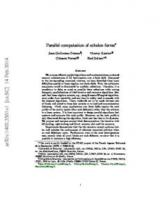
Figure 1. Parallel Computer Organizations
m
. .. ..
(1.2)
(1.3)
m
. .. ..
. .. ..
. .. ..
. .. ..
m
m
. .. ..
m
Figure 1 schematically shows the organization of several parallel computers that have been built over the years. Circles in the Figure represent a node which might consist of a processor, some memory, and a switch. The memory in a node is commonly referred to as the local memory of the processor in the node. Nodes are connected together by communication links, represented by lines in the Figure. One or several nodes in the parallel computer are typically connected to a host, which is a standard sequential computer, e.g. a PC. Users control the parallel computer through the host. Figure 1.1 shows an organization called a two dimensional array, i.e. the nodes can be thought of as placed at integer cartesian coordinates in the plane, with neighboring nodes connected together by a communication link. This is a very popular organization, because of its simplicity, and as we will see, because of the ease of implementing certain algorithms on it. It has been used in several parallel computers, including The Paragon parallel computer built by Intel Corporation. Higher dimensional arrays are also used. For example, the Cray T3E parallel computer as well as the IBM Blue Gene computer are interconnected as a 3 dimensional array of processors illustrated in Figure 1.2. Figure 1.3 shows the binary tree organization. This has been used in several computers e.g. the Database Machine parallel computer built by Teradata Corporation, or the Columbia University DADO experimental parallel computer. Besides two and three dimensional arrays and binary trees, several other organizations have been used for interconnecting parallel computers. Comprehensive descriptions of these can be found in the references given at the end.
1.1.1
Basic Programming Model
A parallel computer can be programmed by providing a program for each processor in it. In most common parallel computer organizations, a processor can only access its local memory. The program provided to each processor may perform operations on data stored in its local memory, much as in a conventional single processor computer. But in addition, processors in a parallel computer can also send and receive messages from processors to which they are connected by communication links. So for example, each processor in Figure 1.1 can send messages to upto 4 processors, the ones in Figure 1.2 to upto 6 processors, and in Figure 1.3 to upto 3 processors. For estimating the execution time of the programs, it is customary to assume that the programs can perform elementary computational operations (e.g. addition or multiplication) on data stored in local memory in a single step. It is also customary to assume that it takes a single time step to send one word of data to a neighboring processor.1 In order to solve an application problem on a parallel computer we must divide up the computation required among the available processors, and provide the programs that run on the processors. How to divide up the computation, and how to manage the communication among the processors falls under the subject of parallel algorithm design. This is explored in the following section. How the programs for the individual processors are expressed by the user, is a question concerning parallel programming languages, these are discussed in Section 1.3. 1
If a processor needs to send a message to a processor that is not directly connected to it, the message must be explicitly forwarded through the intermediate processors. In some parallel computers the switches are intelligent and can themselves forward the messages without involving the main processors. In such computers, more complex models are needed to estimate the time taken for communication.
1.2
Parallel Algorithm Design
Parallel algorithm design is a vast field. Over the years, parallel algorithms have been designed for almost every conceivable computational problem. Some of these algorithms are simple, some laborious, some very clever. I will provide a very brief introduction to the field using three examples: matrix multiplication, a problem called prefix computation, and the problem of selecting the rth largest from a given set of n numbers. These three examples will in no way cover the variety of techniques used for parallel algorithm design, but I hope that they will illustrate some of the basic issues. One strategy for designing a parallel algorithm is to start by understanding how the problem might have been solved on a conventional single processor computer. Often this might reveal that certain operations could potentially be performed in parallel on different processors. The next step is to decide which processor will perform which operations, where input data will be read and how the data structures of the program will be stored among the different processors. For high performance, it is desirable that (1) no processor should be assigned too much work– else that processor will lag behind the others and delay completion (2) The processors should not have to waste time waiting for data to arrive from other processors: whatever data is needed by them should ideally be available in their local memories, or arrive from nearby processors. The algorithms we present for matrix multiplication and for selection essentially use this strategy: the operations in well known sequential algorithms are mapped to the different processors in the parallel computer. Sometimes, however, the natural algorithm used on single processors does not have any operations that can be performed in parallel. In this case we need to think afresh. This is needed in the algorithm for prefix computation. When designing parallel algorithms, an important question to be considered is which model to use. Often, it is useful to start by considering the most convenient model. Once we have an algorithm for one model, it may be possible to simulate it on other models.
1.2.1
Matrix Multiplication
I shall consider square matrices for simplicity. The sequential program for this problem is shown in Figure 2. The program is very simple: it is based directly on the definition of matrix multiplication P (cij = k aik bkj ). More sophisticated algorithms are known for matrix multiplication, but this is the most commonly used algorithm. It is clear from the code that all the n2 elements of C can be calculated in parallel! This idea is used in the parallel program given in Figure 3. An n × n two dimensional array of processors is used, with processors numbered as shown. All processors execute the program shown in the figure. Notice that each basic iteration takes 3 steps (after data is ready on the communication links), I will call this a macrostep. Matrix B is fed from the top, with processor 1i receiving column i of the matrix, one element per macrostep, starting at macrostep i. Processor 11 thus starts receiving its column in macrostep 1, processor 12 in macrostep 2, and so on. This is suggested in Figure 3 by staggering the columns of B. Likewise, matrix A is fed from the left, with processor j1 receiving row j, one element per macrostep, starting at macrostep j. The code for each processor is exceedingly simple. Each processor maintains a local variable z, which it initializes to zero. Then the following operations are repeated n times. Each processor waits until data is available on the left and top links. The numbers read on the two links are multiplied and the product added to the local variable z. Finally,
--------------------------------------------------procedure matmult(A,B,C,n) dimension A(n,n),B(n,n),C(n,n) do i=1,n do j=1,n C(i,j)=0 do k=1,n C(i,j)=C(i,j)+A(i,k)*B(k,j) enddo enddo enddo end --------------------------------------------------Figure 2. Sequential Matrix Multiplication the data read on the left link is sent out on the right link, and the data on the top sent to the bottom link. I will show that processor ij in the array will compute element C(i, j) in its local variable z. To see this notice that every element A(i, k) gets sent to every processor in row i of the array. In fact, observe that processor ij receives elements A(i, k) on its left link at macrostep i + j + k − 1. Similarly processor ij also receives B(k, j) on its top link at the same step! Processor ij multiplies these elements, and notice that the resulting product A(i, k) ∗ B(k, j) is accumulated in its local variable z. Thus it may be seen that by macrostep i + j + n − 1, processor ij has completely calculated C(i, j). Thus all processors finish computation by macrostep 3n − 1 (the last processor to finish is nn). At the end every processor ij holds element C(i, j). The total time taken is 3n − 1 macrosteps (or 9n − 3 steps), which is substantially smaller than the approximately cn3 steps required on a sequential computer (c is a constant that will depend upon machine characteristics). The parallel algorithm is thus faster by a factor proportional to n2 than the sequential version. Notice that since we only have n2 processors, the best we can expect is a speedup of n2 over the sequential. Thus the algorithm has acheived the best time to within constant factors. At this point, quite possibly the readers are saying to themselves, “This is all very fine, but what if the input data was stored in the processors themselves, e.g. could we design a matrix multiplication algorithm if A(i, j) and B(i, j) were stored in processor ij initially and not read from the outside?” It turns out that it is possible to design fast algorithms for this initial data distribution (and several other natural distributions) but the algorithm gets a bit more complicated.
1.2.2
Prefix computation
The input to the prefix problem is an n element vector x. The output is an n element vector y where we require that y(i) = x(1) + x(2) + · · · + x(i). This problem is named prefix computation because we compute all prefixes of the expression x(1) + x(2) + x(3) + · · · + x(n). It turns out that prefix computation problems arise in the design of parallel algorithms for sorting, pattern matching
44
CODE FOR EVERY PROCESSOR local x,y,z,i z=0 do i = 1 to n Receive data on top and left links x = data read from left link y = data read from top link z = z + x*y Transmit x on right link, y on bottom link enddo
34
43
24
33
42
14
23
32
41
13
22
31
12
21 B ?
11
43
41
31
21
42
32
22
12
33
23
13
11
m
m
m
m
m
m
m
m
m
m
m
m
m
m
m
m
A44
34
24
14
Figure 3. Parallel Matrix Multiplication
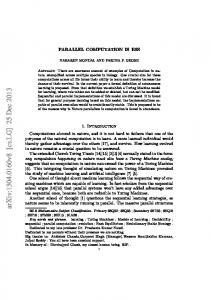
--------------------------------------------------procedure prefix(x,y,n) dimension x(n),y(n) y(1) = x(1) do i=2,n y(i) = y(i-1) + x(i) enddo end --------------------------------------------------Figure 4. Sequential Prefix Computation and others, and also in the design of arithmetic and logic units (ALUs). On a uniprocessor, the prefix computation problem can be solved very easily, in linear time, using the code fragment shown in Figure 4. Unfortunately, this procedure is inherently sequential. The value y(i) computed in iteration i depends upon the value y(i − 1) computed in the i − 1th iteration. Thus, if we are to base any algorithm on this procedure, we could not compute elements of y in parallel. This is a case where we need to think afresh. Thinking afresh helps. Surprisingly enough, we can develop a very fast parallel algorithm to compute prefixes. This algorithm called the parallel prefix algorithm, is presented in Figure 5. It runs on a complete binary tree of processors with n leaves, i.e. 2n − 1 processors overall. The code to be executed by the processors is shown in Figure 5. The code is different for the root, the leaves, and the internal nodes. As will be seen, initially all processors except the leaf processors execute receive statements which implicitly cause them to wait for data to arrive from their children. The leaf processors read in data, with the value of x(i) fed to leaf i from the left. The leaf processors then send this value to their parents. After this the leaves execute a receive statement, which implicitly causes them to wait until data becomes available from their parents. For each internal node, the data eventually arrives from both children. These values are added up and then sent to its own parent. After this the processors wait for data to be available from their parent. The root waits for data to arrive from its children, and after this happens, sends the value 0 to the left child, and the value received from its left child to its right child. It does not use the value sent by the right child. The data sent by the root enables its children to proceed further. These children in turn execute the subsequent steps of their code and send data to their own children and so on. Eventually, the leaves also receive data from their parents, the values received are added to the values read earlier and output. Effectively, the algorithm runs in two phases: in the “up” phases all processors except the root send values towards their parent. In the “down” phase all processors except the root receive values from their parent. Figure 6 shows an example of the algorithm in execution. As input we have used x(i) = i2 . The top picture shows values read at the leaves and also the values communicated to parents by each processor. The bottom picture shows the values sent to children, and the values output. Figure 6 verifies the correctness of the algorithm for an example, but it is not hard to do
--------------------------------------------------procedure for leaf processors local val, pval read val send val to parent Receive data from parent pval = data received from parent write val+pval end --------------------------------------------------procedure for internal nodes local lval, rval, pval Receive data from left and right children lval = data received from left child rval = data received from right child send lval+rval to parent Receive data from parent pval = data received from parent send pval to left child send pval+lval to right child end --------------------------------------------------procedure for root local lval, rval Receive data from left and right children lval = data received from left child rval = data received from right child send 0 to left child send lval to right child end ---------------------------------------------------
Figure 5. Parallel Prefix Computation
m . �� HH � HH 174 � 30 � HH � H ��
�� m . " b b 25 5 "" b " bb " m m 1 �� BB 4 9 �� BB 16 � B. m � B. m m m 6
1
6
4
6
9
HH H m . " b " b 113 61 " b " bb " m m
25 �� BB 36 � m
B. m
6
6
16
25
49 �� BB 64 � m
B. m
6
6
6
36
49
64
m � .H � HH � 0 �� HH30 � H � HH � � HH � m m . . b " " b " " b 5 b 91 0 " 30 " b b " " b bb b " " m m m m 0 �� BB 1 5 �� BB 14 30 �� BB 55 91 �� BB 140 � B. m � B. m � B. m � B. m m m m m . ?
1
?
5
. ?
?
?
?
14
30
55
91
?
?
140
204
Figure 6. Execution Example for Parallel Prefix
so in general. The two main insights are (a) Each internal node sends to its parent the sum of the values read in its descendant leaves, and (b) Each non root node receives from its parent the sum of the values read to the left of its descendant leaves. Both these observations can be proved by induction. In the “up” phase, the leaves are active only in the first step, their parents only at step 2, their parents in turn only at step 3, and so on. The root receives values from its children in step log n, and sends data back to them at step (log n) + 1. This effectively initiates the “down” phase. The down phase mirrors the up phase in that activity is triggered by the root, and the leaves are the last to get activated. Thus the entire algorithm finishes in 2 log n steps. Compare this to the sequential algorithm which took about n steps to complete. 2 log n is much smaller!2 In conclusion even though at first glance it seemed that prefix computation was inherently sequential, it was possible to invent a very fast parallel algorithm.
1.2.3
Selection
On a single processor, selection can be done in O(n) time using deterministic as well as randomized algorithms. The deterministic algorithm is rather complex, and the randomized rather simple. Here we will build upon the latter. The basic idea of the randomized algorithm is: a randomly choose one of the numbers in the input as a splitter. Compare all numbers to the splitter and partition them into 3 sets: those which are larger than the splitter, those which are equal to the splitter, and those that are smaller than the splitter. The problem of finding the rth smallest from the original set can now be reduced to that of finding the r0 th smallest from one of the sets, which set to consider and the value of r0 can both be determined by finding the sizes of the three sets. We next describe the parallel algorithm. For even modestly complicated algorithms, we will typically not write the code for each processor as in the previous examples, but instead present a global picture. This includes the description of what values will be computed (even intermediate values) on which processors, followed by a description of how those values will be computed. The latter will often be specified as a series of global operations, e.g. “copy the value x[1] in processor 1 to x[i] in all processors i”, or “generate array y by performing the prefix operation over the array x”. Of course, this way of describing the algorithm is only a convenience, it is expected that from such a description it should be possible to construct the program for each processor. The parallel algorithm will also run on a tree of processors with n leaves. The input, a[1..n] will initially be stored such that a[i] is on the ith leaf, and r on the root. The algorithm is as follows. 1. Construct an array active[1..n] stored with active[i] on processor i initialized to 1. This is used for keeping track of which elements are active in the problem being solved currently. 2. Next, we pick a a random active element as a splitter as follows: (a) First the rank array is constructed, again with rank[i] on leaf i. This simply numbers all active elements from 1 to however many active elements there are. This is simply 2
We can devise an algorithm that runs in essentially the same time using only p = n/ log n processors. This algorithm is more complex than the one described, but it is optimal in the sense that it is faster than the sequential version by about a factor p.
done by running a prefix over the array a[1..n]. Note that rank is also defined for non active elements, but this is ignored.3 (b) Note now that rank[n] will equal the number of active elements. This value is also obtained at the root as a part of the prefix computation. Call this value Nactive. The root processor picks a random integer srank between 1 and Nactive. This integer is sent to its children, and so on to all the leaves. Each leaf i checks the value it receives, and if active[i]=1 and rank[i]=srank then it sets splitter=a[i]. Notice that only one leaf i will set splitter=a[i]. This leaf sends the value back to the root. 3. Next we compute the number of elements which are smaller than the leaf. For this the root sends splitter to all leaves. Each leaf i sets val[i]=1 if a[i]= splitter. Similarly if r T , then it means that the value output by p is the same no matter what is read in u. This cannot be
possible, and hence Then, T ≥ d(p, u) for all u ∈ G Now, suppose diameter D = d(x, y). Thus D = d(x, y) ≤ d(x, P ) + d(P, y) ≤ 2T . Notice that this also applies to prefix computation, since the last value in the prefix is simply the sum of all elements. For a sequential array, we find that the diameter is N - 1. So, any algorithm using a sequential array of N processors will run in time T ≥ (N − 1)/2. So we can’t do better than O(N ) with such a network, if each processor reads at least one value.1
2.4.3
Bisection Width Bound
Given a graph G = (V, E), where |V | = n, its bisection width is the minimum number of edges required to separate it into subgraphs G1 and G2 , each having at most dn/2e vertices. The resulting subgraphs are said to constitute the optimal bisection. As an example, the bisection width of a complete binary tree on n nodes is 1. To see this, note that at least one edge needs to be removed to disconnect the tree. For a complete binary tree one edge removal also suffices: we can remove one of the edges incident at the root. To see the relevance of bisection width bounds, we consider the problem of sorting. As input we are given a sequence of keys x = x1 , . . . , xn . The goal is to compute a sequence y = y1 , . . . , yn , with the property that y1 ≤ y2 ≤ . . . ≤ yn such that y is a permutation of x. First, consider the problem of sorting on n node complete binary trees. We will informally argue that sorting cannot be performed easily on trees. For this we will show that given any algorithm A there exists a problem instance such that A will need a long time to sort on that instance. We will assume for simplicity that each node of the tree reads 1 input key, and outputs one key. We cannot of course dictate which input is read where, or which output generated where. This is left to the algorithm designer; however, we may assume that input and output are oblivious. Consider any fixed sorting algorithm A. Because input-output is oblivious, we know that the processor where each yi is generated (or xi read) is fixed independent of the input instance. Consider the left subtree of the root. It has m = n − 1/2 processors, with each processor reading and generating one key. Let yi1 , yi2 , . . . , yim be the outputs generated in the left subtree. The right subtree likewise has m processors and reads in m inputs. Let xj1 , xj2 , . . . , xjm be the inputs read in the right subtree. No consider a problem instance in which xj1 is set to be the i1 th largest in the sequence x, xj2 is set to be the i2 th largest, and so on. Clearly, to correctly sort this sequence, all the keys read in the right subtree will have to be moved to the left subtree. But all of these keys must pass through the root! Thus, just to pass through the root the time will be O(m) = O(n). Sequential algorithms sort in time O(n log n), thus the speedup is at most O(log n) using n processors.2 In general, the time for sorting is Ω(n/B), where B is the bisection width of the network. 1
Suppose, however, that we use only p processors out of the N . Now we can apply the theorem to the subgraph induced by the processors which read in values. Then the speedup bound is N/p, and the diameter bound is (p−1)/2. √ √ So, T ≥ (N/p, (p − 1)/2). This can be minimized by taking p = O( N ), √ √so that both lower bounds give us O( N ). This bound can √ be easily matched: read N values on each of the first N processors. Processors compute the sum locally in O( N ) time, and then add the values together also in the same amount of extra time. 2 Can we somehow compress the keys as they pass through the bisection? If the keys are long enough, then we cannot, as we will see later in the course. For short keys, however, this compression is possible, as seen in the exercises.
Notice that the diameter is also a lower bound for sorting: it is possible that a key must be moved between points in the network that define the diameter. However, sometimes the diameter bound will be worse than bisection, as is the case for trees.
2.5
Exercises
1. We argued informally that the root of the tree constituted a bottleneck for sorting. This argument assumed that all the keys could have to pass unchanged through. An interesting question is, can we some how “compress” the information about the keys on the right rather than explicitly send each key? It turns out that this is possible if the keys are short. (a) Show how to sort n keys each 1 bit long in time O(log n) on an n leaf complete binary tree. (b) Extend the previous idea and show how to sort n numbers, each log log n bits long, in time O(log n). Assume in each case that the processors can operate on log n bit numbers in a single step, and also that log n bit numbers can be sent across any link in a single step. 2. Consider the problem of sorting N keys on a p processor complete binary tree. Give lower bounds based on speedup, diameter, and bisection width.
Chapter 3 More on prefix First, note that the prefix operation is a generalization of the operations of broadcasting and accumulation defined as follows. Suppose one processor in a parallel computer has a certain value which needs to be sent to all others. This operation is called a broadcast operation, and was used in the preceding lecture in the selection algorithm. In an accumulate operation, every processor has a value, which must be combined together using a single operator (e.g. sum) into a single value. We also saw examples of this in the previous lecture. We also saw the prefix operation over an associative operator “+”. Indeed, by defining a + b = a we get a broadcast operation, and the last element of the the prefix is in fact the accumulation of the inputs. Thus the prefix is a generalization of broadcasting as well as accumulation. We also noted that these operations can be implemented well on trees. The prefix operation turns out to be very powerful. when x[1..n] is a bit vector and + represents exclusive or, the prefix can be used in carry look ahead adders. Another possibility is to consider + to be matrix multiplication, with each element of x being a matrix. This turns out to be useful in solving linear recurrences, as will be seen in an exercise. The algorithm can also be generalized so that it works on any rooted tree, not just complete binary trees. All that is necessary is that the leaves be numbered left to right. It is easy to show that if the degree of the tree is d and height h, then the algorithm will run in time O(dh).
3.1
Recognition of regular languages
A language is said to be regular if it is accepted by some deterministic finite automaton. The problem of recognizing regular languages commonly arises in lexical analysis of programming languages, and we will present a parallel algorithm for this so called tokenization problem. Given a text string, the goal of tokenization is to return a sequence of tokens that constitute the string. For example, given a string if x yk+1 for some k. We will 30
show that the algorithm will also make an error when presented with the sequence f (x1 ), . . . , f (xN ), where (
f (x) =
0 1
if x < yk otherwise
To see this let xit , Xit respectively denote the value in A[i] after step t for the two executions considered, i.e first with input x1 , . . . , xn and second with input f (x1 ), . . . , f (xn ). We will show by induction on t that Xit = f (xit ); this is clearly true for the base case t = 0. Suppose this holds at t. Let the instruction in step t + 1 be OCE(i, j). If xit ≤ xjt then there will be no exchange in the first execution. The key point is that f is monotinic. We thus have that f (xit ) ≤ f (xjt ), and hence by the induction hypothesis we also must have Xit ≤ Xjt . Thus there will be no exchange in the second execution also. If on the other hand, xit > xjt , then there is an exchange in the first execution. In the second iteration, we must have either (a) Xit > Xjt , in which case there is an exchange in the second iteration as well, or (b) Xit = Xjt in which case there really is no exchange, but we might as well pretend that there is an exchange in the second execution. From the above analysis we can conclude that sequence output in the second execution will be f (y1 ), . . . , f (yn ). But we know that f (yk ) = 1 and f (yk+1 ) = 0. Thus we have shown that the algorithm does not correctly sort the 0-1 sequence f (x1 ), . . . , f (xN ). But since the algorithm was supposed to sort all 0-1 sequences correctly it follows that it could not be making a mistake for any sequence x1 , . . . , xn . Remark: Sorting a general sequence is equivalent to ensuring for all i that the smallest i elements appear before the others. But in order to get the top i to appear first, we dot need to distinguish between them, i.e. we only need to distinguish between the top i and the rest. An algorithm that correctly sorts all arbitrary sequence of i 0s and rest 1s will in fact ensure that the smallest i elements in a general sequence will go to the front.
5.3
The Delay Sequence Argument
While investigating a phenomenon, a natural strategy is to look for its immediate cause. For example, the immediate cause for a student failing an examination might be discovered to be that he did not study. While this by itself is not enlightening, we could persevere and ask why did he not study, to which the answer might be that he had to work at a job. Thus an enquiry into successive immediate causes could lead to a good explanation of the phenomenon. Of course, this strategy may not always work. In the proverbial case of the last straw breaking the camel’s back, detailed enquiry into why the last straw was put on the camel (it might have flown in with the wind) may not lead to the right explanation of why the camel’s back broke. Nevertheless, this strategy is often useful in real life, and as it turns out, also in the analysis of parallel/distributed algorithms. In this context it has been called the Delay Sequence Argument. The delay sequence argument may be thought of as a general technique for analyzing a process defined by events which depend upon one another. The process may be stochastic; either because it employs randomized algorithms or because its definition includes random input. The technique works by examining execution traces of the process1 . An execution trace is simply a record of the 1
Sort of a post mortem..
computational events that happened during execution, including associated random aspects. The idea is to characterize traces in which execution times are high, and find a critical path of events which are responsible for the time being high. If the process is stochastic, the next step is to show that long critical paths are unlikely – we will take this up later in the course. The process we are concerned with is a computational problem defined by a directed acyclic graph. The nodes represent atomic operations and edges represent precedence constraints between the atomic operations. For example, in the sorting problem, an event might be the movement of a key across a certain edge in the network. Typically, the computational events are related, e.g. in order for a key to move out of a processor, it first has to get there (unless it was present there at the beginning of the execution). The parallel algorithm may be thought of as scheduling these events consistent with the precedence constraints. An important notion is that of a Enabling Set of a (computational) event. Let T0 denote a fixed integer which we will call the startup time for the computation. We will say Y is a enabling set for event x iff the occurrence of x at time t > T0 in any execution trace guarantees the occurrence of some y ∈ Y at time t − 1 in that execution trace. We could of course declare all events to be in the enbaling set of every event – this trivially satisfies our definition. However it is more interesting if we can find small enabling sets. This is done typically by asking “If x happened at t, why did it not happen earlier? Which event y happening at time t − 1 finally enabled x to happen at t?” The enabling set of x consists of all such events y. A delay sequence is simply a sequence of events such that the ith event in the sequence belongs to the enabling set of the i + 1th event of the sequence. A delay sequence is said to occur in an execution trace if all the events in the delay sequence occur in that trace. Delay sequences are interesting because of the following Lemma. Lemma 2 Let T denote the execution time for a certain trace. Then a delay sequence E = ET0 , ET0 +1 , . . . , ET occurs in that trace, with event Et occurring at time t. Proof: Let ET be any of the events happening at time T . Let ET −1 be any of the events in the enabling set of ET that is known to have happened at time T − 1. But we can continue in this manner until we reach ET0 . The length of the delay sequence will typically be the same as the execution time of the trace, since typically T0 = 1 as will be seen. Often, the process will have the property that long delay sequences cannot arise (as seen next) which will establish that the time taken must be small.
5.4
Analysis of Odd-even Transposition Sort
Theorem 2 Odd-even transposition sort on an N processor array completes in N steps. The algorithm is clearly oblivious comparison exchange, and hence the Zero-one Lemma applies. We focus on the movement of the zeros during execution. For the purpose of the analysis, we will number the zeros in the input from left to right. Notice that during execution, zeros do not overtake each other, i.e. the ith zero from the left at the start of the execution continues to have exactly
i − 1 zeros to its left throughout execution: if the ith and i + 1th zero get compared during a comparison-exchange step, we assume that the ith is retained in the smaller numbered processor, and the i + 1th in the larger numbered processor. Let (p, z) denote the event that the zth zero (from the left) arrives into processor p. Lemma 3 The enabling set for (p, z) is {(p + 1, z), (p − 1, z − 1)}. The startup time T0 = 2. Proof: Suppose (p, z) happened at time t. We ask why it did not happen earlier. Of course, if t ≤ 2 then this might be the first time step in which the zth zero was compared with a key to its left. Otherwise, the reason must be one of the following: (i) the zth zero reached processor p + 1 only in step t − 1, or (ii) the zth zero reached processor p + 1 earlier, but could not move into processor p because z − 1th zero left processor p only in step t − 1. In other words, one of the events (p + 1, z) and (p − 1, z − 1) must have happened at time t − 1. (p + 1, z) and (p − 1, z − 1) will respectively be said to cause transit delay and comparison delay for (p, z). Proof of Theorem 2: Suppose sorting finishes at some step T . A delay sequence ET0 , . . . , ET with T0 = 2 must have occurred. We further know that Et = (pt , zt ) occurred at time t. Just before the movement happened at step 2, we know that the z2 th zero, the z2 + 1th zero and so on until the zT th zero must all have been present in processors p2 + 1 through N . But this range of processors must be able to accomodate these 1 + zT − z2 zeros. Thus N − p2 ≥ 1 + zT − z2 . Let the number of comparison delays in the delay sequence be c. For every comparison delay, we have a new zero in the delay sequence, i.e. c = zT − z2 . Further, a transit delay of an event happens to its right, while a comparison delay to its left. Thus from pT to p2 we have T − 2 − c steps to the right, and c steps to the left, i.e. p2 − pT = T − 2 − 2c. Thus T = p2 − pT + 2 + 2c = p2 − pT + 2 + 2zT − 2z2 ≤ N − pT + 1 + zT − z2 Noting that pT = zT and z2 ≥ 1 the result follows.
Chapter 6 Systolic Conversion An important feature of designing parallel algorithms on arrays is arranging the precise times at which operations happen, and also the precise manner in which the input/output have to be staggered. We saw this for matrix multiplication. The main reason for staggering the input was the lack of a broadcast facility. If we had a suitable broadcast facility, the matrix multiplication algorithm could be made to look much more obvious. As shown, we could simply broadcast row k of B and column k of A, and each processor (i, j) would simply accumulate the product aik bkj at step k, and the whole algorithm would finish in n steps. This algorithm is not only fast, but is substantially easier to understand. Unfortunately, broadcasts are not allowed in our basic model. The reason is that sending data is much faster over point to point links than over broadcast channels, where the time is typically some (slowly growing) function of the number of receivers. All is not lost, however. As it turns out, we can take the more obvious algorithm for matrix multiplication that uses broadcasts, and automatically transform it into the algorithm first presented. Thus, the automatic transformation, called systolic conversion allows us to specify algorithms using the broadcast operation and yet have our algorithm get linear speedup when run on a network that does not allow broadcast operations! In fact using systolic conversion, we can do more than just broadcasting. To put very simply, during the process of designing the algorithm, we are allowed to include in our network special edges which have zero delay. Strange as this may seem, a signal sent on such edges arrives at the destination at the beginning of the same step in which it was sent, and the data received can in fact be used in the same cycle by the receiving processor! Using the systolic conversion theorem we can take algorithms that need the special edges and from them generate algorithms that do not need zero delay. Of course, the special edges cannot be used too liberally– we discuss the precise restrictions in the next lecture. But for many problems, the ability to use zero delay edges during the process of algorithm design substantially simplifies the process of discovering the algorithm as well as specifying it. Before describing systolic conversion, we present one motivating example.
6.1
Palindrome Recognition
Suppose we are given as input a string of characters x1 , x2 , . . . , x2n , where xi is presented at step i. We are required to design a realtime palindrome recognizer, i.e. our parallel computer should
34
indicate by step 2j + 1 for every j whether or not the string x1 , . . . , x2j is a palindrome (i.e. whether x1 = x2j and x2 = x2j−1 and so on). Shown is a linear array of n processors for solving this problem. It uses ordinary (delay 1) edges, as well as the special zero delay edges. The algorithm is extremely simple to state. In general, for after any step 2j, the array holds the string x1 , . . . , x2j in a folded manner in the first j processors. Processor i holds xi and x2j+1−i ; these are precisely two of the elements that need to be equal to check if x2j is a palindrome. Using the 0 delay edges, processor j sends the result of its comparison to processor j − 1. Processor j − 1 receives it in the same step, “ands” it with the result of its own comparison and sends it to processor j − 2 and so on. As a result of this, processor 1 generates a value “true” if the string is a palindrome, and “false” otherwise, all in the very same step!! The rest of the algorithm is easily guessed. In steps 2j + 1, the inputs x2j , . . . , xj+1 are shifted one spot to the right. Input x2j+1 arrives into processor 1. The zero delay edges are not used in this step at all. In step 2j + 2, elements x2j+1 , . . . , xj+2 moves one spot to the right and element x2j+2 arrives into processor 1. As described above, each processor compares the elements it has, and the zero delay edges are used to compute the conjuction of the comparison results. Thus at the end of step 2j + 2, the array determines whether or not x1 , . . . , x2j+2 is a palindrome. Two points need to be made about this example. First, the zero delay edges seem to provide us with more power here than in the matrix multiplication example: they are actually allowing us to perform several “and” computations in a single step. The second point is that the algorithm above is very easy (trivial!) to understand. It is possible to design a palindrome recognition algorithm without using zero delays, but it is extremely complicated, the reader is encouraged to try this as an exercise.
6.2
Some terminology
A network is represented by a directed graph G(V, E). Each vertex represents a processor with edges representing communication channels. Each edge is associated with a non-negative integer called its delay. Some vertex in the graph is designated the host. Only the host is assumed to communicate with the external world. During each step each processor does the following (1) wait until the values arriving on its input edges stabilize, (2) executes a single instruction using its internal state or the values on the input edges, and (3) possibly modify its internal state or write values onto the outgoing edges. The value written on an edge e at step t arrives into the processor into which e is directed at step t + delay(e). Notice that if delay(e) > 1 then an edge effectively behaves like a shift register. A network is semisystolic if there are no directed cycles with total delay of zero: ∀ C ∈ G,
X
delay(e) > 0.
e∈C
The requirement for a systolic network is that ∀ e ∈ E, delay(e) > 0. The palindrome recognition network and the second matrix multiplication network presented in the last lecture were semisystolic; all other networks seen in this module were systolic. We will say that a network S is equivalent to a network S0 if the following hold: (1) they have the same graph; (2) corresponding nodes execute the same computations, though a node in one
network may lag the corresponding node in the other in time by a constant number of steps; (3) the behavior seen at the host is identical.
6.3
The main theorem
Theorem 3 Given semisystolic network S we can transform it to an equivalent systolic network S0 iff for every directed cycle C in S0 we have: |C| ≤
X
delay(e)
e∈C
where |C| denotes the length of the cycle C. We shall transform S to S0 by applying a sequence of basic retiming steps. If we have a network that is semisystolic, but for which some cycle has a smaller total delay than its length, then we can still apply the above theorem after slowing down the network (section 6.8).
6.4
Basic Retiming Step
A positive basic retiming step is applied to a vertex as follows. Consider a vertex with delays i1 , i2 , . . . on its incoming edges and o1 , o2 , . . . on its outgoing edges. Suppose all the delays on the outgoing edges are larger than one. Suppose we remove one delay from every output and add one delay to the input. Suppose further that that the program for the vertex is made to execute one step later than before i.e. it executes the same instructions, but each instruction is executed one step later than before. Negative retiming steps are defined similarly. It is clear that the behavior of the network does not change because of retiming. First the values computed by the retimed vertex do not change—it does receive its inputs one step late but its program is also delayed by one step. But although the vertex produces values late, the rest of the graph cannot discover this since one delay has been removed from the outputs of the vertex, so they arrive to other vertices at precisely the right times.
6.5
The Lag Function
We shall construct a function lag(u) for each node u that will denote the total number of delays that are moved from outgoing edges of node u to the incoming edges during some sequence of retiming operations. Note that lag(u) also denotes the number of timesteps the program of u is delayed. Because of the retiming, the delay for an edge uv ~ will increase by an amount lag(v), since that many delays are moved in, and decrease by lag(u), since that many delays are moved out. Thus we will have newdelay(uv) ~ = delay(uv) ~ + lag(v) − lag(u). To prove the theorem we must show that • newdelay(uv) ~ > 0, ∀ (u, v) ∈ E. • lag(host) = 0, since the external behavior would change if we moved delays across the host. • There exists a sequence of retiming steps such that the required number of delays can be moved across each vertex. Remember that we cannot let the delay for any edge go down below zero during the retiming process.
6.6
Construction of lags
Consider any path P from a vertex u to the host. After retiming, the total number of delays along the path must be greater than the length of the path. The total number of delays that are moved out of the path during retiming is lag(u), since nothing is moved in through the host. Thus we must have ! X
delay(e) − lag(u) ≥ |P |
e∈P
Or alternatively, lag(u) ≤
X
(delay(e) − 1)
e∈P
We will define a new graph which we will call G − 1, which is same as G, except that each edge delay is reduced by 1. Think of this as the “surplus graph”; the delays in G − 1 indicate how many surplus registers the edge has for moving out. We will call the delay of an edge in G − 1 its surplus. Further, for any path P define surplus(P ) to be the sum of the surpluses of its edges. The expression above simply says that lag(u) ≤ surplus(P ). Our choice of the lags must satisfy this for all possible paths P from u to the host. In fact it turns out that this choice is adequate. In particular we choose lag(u) ≡ min{surplus(P )| P is a path from u to host.} P
In other words, we compute the lag for each node as the shortest distance from it to the host. In P G we knew for any cycle C that e∈C delay(e) ≥ |C|. Thus G − 1 does not have negative cycles, thus our lag function is well defined.
6.7
Proof of theorem
We show that the lag function defined above satisfies the three properties mentioned earlier. 1. First we show that newdelay(uv) ~ = delay(uv) ~ + lag(v) − lag(u) > 0 for every edge uv. ~ Let P denote a path from v to the host such that lag(v) = surplus(P ); we know that some such path must exist by the definition of lag. Let P 0 denote the path from u to the host obtained by adding uv ~ to P . By the definition of lag, we have:
lag(u) ≤ surplus(P 0 ) = surplus(uv) ~ + surplus(P ) = delay(uv) ~ − 1 + lag(v) From this we get newdelay(uv) ~ > 0 as needed. 2. The lag of the host is 0 by construction. 3. Now we show that the lags as computed as above can actually be applied using valid basic retiming steps.
We start with lag(u) computed as above for every vertex u. We shall examine every vertex in turn and apply a basic retiming steps if possible. Specifically we apply a positive (negative) retiming step to a node u if (1) lag(u) is greater (less) than 0, and (2) all the delays on the outgoing (incoming) edges are greater than 0. If it is possible to apply a retiming step, we do so, and decrement (increment) lag(u). This is repeated as long as possible. The process terminates if (a) All the lags are down to zero, in which case we are done. (b) There exists some u with lag(u) > 0, but for every such vertex we have some outgoing edge uv ~ with delay(uv) ~ = 0, so that the basic retiming step cannot be applied. But we knew in S that lag(v) ≥ lag(u) + 1 − delay(uv). ~ This inequality is maintained by the application of the basic retiming steps. Thus we get lag(v) ≥ lag(u) + 1, since we currently have delay(uv) ~ = 0. Thus starting at u and following outgoing edges with zero delay, we must be able to find an unending sequence of nodes whose lag is greater than 0. Since the graph is finite, this sequence must revisit a node. But we have then found a directed cycle with total delay equal to 0. Since the basic retiming steps do not change the delay along a cycle, this cycle must have also existed in S, giving a contradiction. (c) There exists some u with lag(u) < 0, but for every such vertex we have some incoming edge uv ~ with delay(uv) ~ = 0, so that the basic retiming step cannot be applied. We obtain a contradiction as in the previous case. Thus the process terminates only after we have applied all the required retiming steps, proving the existence of such a sequence.
6.8
Slowdown
If we have a network that is semisystolic, but for which some cycle has a smaller total delay than its length, then we slow down the execution of the network, i.e. slow down the execution of every component. This effectively increases the delay in each cycle. By choosing a suitable slowdown factor, we can always obtain enough delay so that the systolic conversion theorem can be applied.
6.9
Algorithm design strategy summary
The algorithm design has the following steps. 1. Design an algorithm for a semisystolic network, G. 2. For each cycle C of G, let sC = d|C|/delayCe. Let s = maxC sC . Slowdown G by a factor s. Call the new network sG. 3. Find lag(u) = weight of shortest path from u to the host in sG − 1. Here, weight = delay in sG − 1. 4. Set newdelay(u, v) = delay(u, v) + lag(v) − lag(u). Note that delay(u, v) is the delay in sG. 5. The resulting network is the systolic network equivalent to G.
6.10
Remark
Besides the ease of discovering algorithms, you will note that the semisystolic model is also easier for describing algorithms. This is also an important reason for designing algorithms using the semisystolic model and then converting it to the systolic model.
Exercises 1. Is it necessary that there be a unique systolic network that is equivalent to a given semisystolic one? Justify or give a counter example. 2. We defined lag(u) to be the length of the shortest path from u to the host. What if there is no such path? 3. We said that the nodes that are lagged need to start executing their program earlier by as many steps as the lag. Does this mean that each processor needs to know its lag? For which kinds of programs will it be crucial whether or not the processors start executing at exactly the right step? For which programs will it not matter?
Chapter 7 Applications of Systolic Conversion We will see two applications of systolic conversion. The first is to palindrome recognition. We will derive a systolic network for the problem by transforming the semistolic network developed earlier. We will then design a semisystolic algorithm for computing the transitive closure of a graph. We will show how this design can be transformed to give a systolic algorithm. We will mention how other problems like shortest paths and minimum spanning trees can also be solved using similar ideas.
7.1
Palindrome Recognition
To apply the systolic conversion theorem, we need that every cycle in the network have delay at least as large as its length. Unfortunately the semisystolic network we designed does not satisfy this requirement. So we slowdown the original network by a factor of 2. This means that each processor (as well as the host) only operates on alternate steps; each message encounters a 2 step delay to traverse each edge that originally had a delay of 1. Zero delay edges still function instantaneously, as before. With this change, each cycle in the network has delay exactly equal to its length. So we can now apply the systolic conversion theorem. The first step is to compute the surplus for each edge, then the lags are computed by doing the shortest path computation. As will be seen, the processor u at distance i from the host will have shortest path length = −i = lag(u). Now using the formula newdelay(uv) = delay(uv) + lag(v) − lag(u), we will see that each edge will endup with a unit delay. Note that we could also have retimed the network ”by hand”, by moving delays around heuristically. To get started, we move the delay around the farthest processor. As you can see, delays can be moved around so that we will reach the same solution as obtained bt applying the systolic conversion theorem.
7.2
Transitive Closure
Let G = (V, E) be a directed graph. Its transitive closure is the graph G∗ = (V, E ∗ ), where E ∗ = {(i, j)|∃ directed path from i to j in G} Sequentially, transitive closure is computed typically using the Floyd-Warshall algorithm which runs in time O(N 3 ), for an N vertex graph. Faster algorithms exist, based on ideas similar to 40
Strassen’s algorithm for matrix multiplication, but these are considered to be impractical unless N is enormous. We will present a parallel version of the Floyd-Warshall algorithm. It will run on an N 2 processor mesh in time O(N ), thus giving linear speedup compared to the sequential version. Floyd-Warshall’s algorithm effectively constructs a sequence of Graphs G0 , G1 , . . . , GN , where G0 = G and GN = G∗ . Given a numbering of the vertices with the numbers 1, . . . , N , we have Gk = (V, E k ), where E k = {(i, j)|∃ path in G from i to j with no intermediate vertex larger than k} Note that E 0 and E N are consistent with our definition. The algorithm represents each graph Gk using its adjacency matrix Ak . The matrix Ak is computed from Ak−1 using the following lemma. k−1 Lemma 4 akij = ak−1 ∨ (ak−1 ij ik ∧ akj )
Proof: If there is a path from i to j passing through vertices no larger than k then either it passes strictly through vertices smaller than k, or k lies on the path. But in that case there are paths from i to k and from k to j both of which pass through vertices strictly smaller than k. k−1 k−1 k−1 Note a small point which will be needed later akik = aik ∨ (ak−1 ik ∧ akk ) = aik . Thus the ith column of Ak is the same as the ith column of Ak−1 . Similarly, the ith row of Ak is also the same as the ith row of Ak−1 .
7.2.1
Parallel Implementation
The parallel implementation needs a square N × N mesh. We start with a semisystolic network to facilitate the design process. The network receives the matrix A0 = A from the top, fed in one row at each step. The matrix A∗ is generated at the bottom eventually, also one row at each step. The kth row of processors generates the matrix Ak given Ak−1 . Notice the manner in which input is fed; the rows of Ak−1 are fed in the order k, k + 1, k + 2, . . . , N, 1, 2, . . . , k − 1. The rows of Ak are generated in the order k + 1, k + 2, . . . , N, 1, 2, . . . , k, which is precisely the order in which the k + 1th row of processors needs its input. Row k of processors performs its work as follows. The row it first receives, row k of Ak−1 is simply stored; processor kj stores ak−1 kj . Subsequently, some row i is received. Processor kk receives k−1 aik broadcasts it to the all processors kj, and also sends it to processors k + 1, k. Simultaeously processor kj receives ak−1 from the top and ak−1 on the broadcast. Thus it can compute akij = ij ik k−1 ak−1 ∨ (ak−1 ij ik ∧ akj ), which it can pass on to processor k + 1, j. After all rows have been received from the top, it sends out what it has, i.e. row k of Ak−1 , which as we remarked is also the row k of Ak . We next estimate the time taken in this semisystolic model. Row 1 of A0 = A is sent by the host at step 1 and arrives at the first processor row at step 2. Rows are fed 1 per step after that so that row N of A0 arrives at the first processor row in step N + 1. Row N moves down one processor row per step, so that it arrives at processor row N at time 2N . Following that, row 1 arrives into processor row N at step 2N + 1, and row N − 1 at step 3N − 1. Row N − 1 arrives into the lower host at step 3N , following which row N arrives. So the entire computation takes a total of 3N + 1 steps.
7.2.2
Retiming
We first consider the case in which the upper and lower hosts are really a single processor. In this case, it is easily seen that most cycles do not have enough net delay in them. Further, that a slowdown of a factor of 3 suffices. We leave it as an exercise to compute the new delay of each edge; we only note that because of this slowdown, the entire computation will be completed in time 3(3N+1)=9N+3. Another strategy is to consider the lower host as the “real” host, and keep the upper host as a distinct node. This means that the upper host may have a nonzero lag. This will have to be accounted for in estimating the total computation time. As will be seen, if we keep the hosts separate, the graph does not have any cycles. So a slowdown is not necessary. The computation of the lags and delays is left as an exercise again, we only note that the upper host gets assigned a lag of −(2N − 2). In other words, the upper host needs to start its execution at step −(2N − 2) in order that the lower host finishes at step 3N + 1. Thus the computation really takes time 3N + 1 + 2N − 2 = 5N − 1. Notice that this is faster than the previous design which took 9N + 3 steps.
7.2.3
Other Graph Problems
As it turns out, we can use the algorithm developed above with minimal changes to compute shortest paths and minimum spanning trees. For the shortest path problem, we consider A to be edge length matrix, i.e. aij denotes the length of edge (i, j). We use the same array as before, and perform essentially the same computation, but use a different semiring[1, 4]. In particular, we replace the operator ∨ with the operator min (this takes two arguments and returns their minimum), and the operator ∧ with +, the binary addition operator. Minimum spanning trees can also be computed in a similar manner. As before, the input matrix A gives edge lengths. We modify the transitive closure algorithm by replacing ∨ with min and ∧ with max.
Exercises 1. Complete the retiming for the transitive closure networks (with and and without separate hosts). Attempt to rearrange delays so that they are uniformly distributed. 2. Show how to implement a priority queue using a linear array of N processors. The array should accept as input two operations DELETE-MIN and INSERT(x) at one end and in case of DELETE-MIN, the answer (the minimum element in the queue) should be returned at the same end (the minimum element should also be deleted from the array) in time independent of N . The array should function properly so long as the number of elements in the queue at any instant is less than N . 3. Show how to compute the strongly connected components of an N node graph (input presented as an adjacency matrix) on an N × N mesh. The output should be a labelling of vertices, i.e. vertices in each strong component should be assigned a unique label.
4. Suppose you are given a systolic network in which one node is designated the host. The network has been programmed to run some algorithm (that it runs correctly) except that a modification is needed to the algorithm which requires instantaneous broadcast from the host to all processors. This could certainly be achieved by adding additional wires from the host to every other node; but it can be done without changing the network at all, although a slowdown of a factor of 2 is necessary. In other words, show that the in addition to the communication required for the old program, it is possible to perform broadcast from the host at every step if a slowdown of a factor of 2 is allowed. 5. Consider a slightly modified palindrome recognition problem as follows. In this, the host generates the characters x1 , x2 , . . . , xn in order, but there might be a gap of one or more time steps between consecutive xi , rather than the exact one step gap in the original problem. The goal is still the same: devise a circuit which determines whether the characters received till then form a palindrome. Show how to do this.
Chapter 8 Hypercubes The main topic of this lecture is the hypercube interconnection structure. Hypercubes are a very common interconnection structure in parallel processing because of a number of reasons. First, they can effectively simulate the execution of smaller dimensional arrays and trees. Second, they allow the development of a very rich class of algorithms called Normal Algorithms. In this lecture we will define hypercubes and explore its properties. In addition we will also define the notion of graph embedding, which will be useful to develop the relationship between hypercubes and other networks. Normal algorithms will be considered in the following lecture.
8.1
Definitions
An n dimensional hypercube, denoted Hn has 2n vertices labelled 0..2n − 1. Vertex u and v are connected by an edge iff the binary representations of u and v differ in a single bit. We use ⊕ to denote the exclusive or of bitstrings. Thus u and v have an edge iff v = v ⊕ 2k for some integer k. We will say that the edge (u, u ⊕ 2k ) is along dimension k. Another definition of hypercubes expresses it as a graph product.
8.1.1
The hypercube as a graph product
The product G2H of graphs G, H is defined to have the vertex set V (G2H) = the cartesian product V (G) × V (H), and there is an edge from (g, h) to (g 0 , h0 ) in G2H iff (a) g = g 0 and h, h0 are neighbours in H, or (b) h = h0 and g, g 0 are neighbours in G. Clearly, |V (G2H)| = |V (G)| · |V (H)|. Here is a way to visualize a G2H. Consider |V (G)| rows, each containing |V (H)| vertices. Label the rows by labels of vertices V (G), and the columns by Vertices V (H). On the vertices in each row, put down a copy of H, with h in row labelled h. Similarly, in each column, put down a copy of G. This then is the product G2H. It is customary to say that g is the first coordinate of vertex (g, h) of G2H, and h the second. The hypercube is perhaps the simplest example of a product graph. Consider P2 , the path graph on two vertices, i.e. the graph that consists of a single edge. Then H1 = P2 , H2 = H1 2P2 , H3 = H2 2P2 , and so on. If we have a 3 way product, say (F 2G)2H, then each vertex in the result can be assigned a label ((f, g), h). However, as we will see next, graph products are associative, so that we may write the product as just F 2G2H, and the label as (f, g, h). 44
Lemma 5 2 is commutative and associative. Proof: Need to show that G2H is isomorphic to H2G. Recall that X is isomorphic to Y if there exists a bijection f from V (X) to V (Y ) s.t. (x, x0 ) is an edge in X iff (f (x), f (x0 )) is an edge in Y . The vertices in G2H are (g, h) and those in H2G are (h, g) where g ∈ V (G), h ∈ V (H). We use f ((g, h)) = (h, g). There is an edge from (g, h) to (g 0 , h0 ) in G2H ⇔ either (a) g = g 0 and h, h0 are neighbours in H, or (b) h = h0 and g, g 0 are neighbours in G. ⇔ There is an edge from (h, g) to (h0 , g 0 ) in H2G. ⇔ There is an edge from f ((g, h)) = (h, g) to f ((g 0 , h0 )) = (h0 , g 0 ) in H2G. Thus f is the required isomorphism. Associativitity is similar. At this point it should be clear that our new definition of Hn is really the same as the old. Let the vertices in P2 be labelled 0, 1. Then the coordinates in an n-way products will be x0 , x1 , . . . , xn−1 , where each xi is 0 or 1. In the old definition, we merely concatenated these to get a single n-bit string.
8.2
Symmetries of the hypercube
It may be obvious that all vertices of a hypercube are symmetrical, or more formally, that the hypercube is vertex transitive. This is proved using the notion of a automorphism. An automorphism is simply an isomorphism from a graph to itself. It will be convenient to think of vertices as k bit strings. It will also be useful to have the notation u ⊕ v which denotes the bit-wise exclusive or of u and v. Note that ⊕ is associative and commutative, and that the all 0s string is the identity and each element is its own inverse. Further, suppose u, v are neighbours. Thus they must differ in just one bit. Say it is the ith least significant bit. Then we may write u = v ⊕ 2i . We will show that there is an automorphism f on Qk that maps any vertex u to any vertex v. Consider f (x) = x ⊕ w where w = (u ⊕ v). 1. f (x) = f (y) ⇒ x ⊕ w = y ⊕ w ⇒ x ⊕ w ⊕ w = y ⊕ w ⊕ w ⇒ x = y. Thus f is a bijection. 2. f (u) = u ⊕ w = u ⊕ u ⊕ v = v. Thus f maps u to v as required. 3. Consider a vertex x and its neighbour x ⊕ 2i . Then we have f (x ⊕ 2i ) = x ⊕ 2i ⊕ w = x ⊕ w ⊕ 2i = f (x) ⊕ 2i . Thus f (x ⊕ 2i ) and f (x) are also neighbours across dimension i. Thus f is the required automorphism.
8.3
Diameter and Bisection Width
The diameter of an n dimensional hypercube is n. This follows because the shortest distance between u and v is the number of bits in which they differ; and this can be at most n, as is for example when u = 0 and v = 2n − 1. The bisection width of the hypercube is n/2. Clearly, we can disconnect the hypercube into two parts by removing the edges along any one dimension; it is also possible to show that at least n/2 edges must be removed to disconnect the hypercube into subgraphs of n/2 vertices each.
8.4
Graph Embedding
The formalism of graph embedding is useful to describe the simulation of one network (guest) by another (host). Consider a (guest) graph G = (VG , EG ) and a (host) graph H = (VH , GH ). An embedding of G into H : (fV , fE ) is specified by two functions: fV : V G → V H fE : EG → Paths in H with the condition that if (u, v) ∈ G then fE (u, v) is required to be a path from fV (u) to fV (v). Given an embedding we define the following: ∀w ∈ VH : LOAD(w) = | Vertices of G placed on w| ∀e ∈ EG : DILATION(e) = Length of fE (e) ∀e ∈ EH : CONGESTION(e) = |{e0 |e ∈ fE (e0 )}| Finally, we define the LOAD, DILATION and CONGESTION of the embedding to be the maximum values of the respective parameters. Finally, it is customary to implicitly consider embeddings with LOAD=1, unless the LOAD is explicitly stated. Lemma 6 Let l, d, c denote the load, congestion and dilation for embedding network G into network H. Then G can be simulated on H with a slowdown of O(l + d + c). The proof of this lemma in its most general form is beyond the scope of this course, but can be found in [6]. Here we will sketch the proof of a weaker result: we will show that the time is O(l +cd). First, consider the simulation of the computation steps of G. Each processor of H does the work of at most l processors of G, and hence a step containing only computation can be simulated on H in time O(l). A communication step of G is simulated by sending messages in H along the paths of fE . Consider any such message. The message moves at most d edges of H, and can be delayed during the movement at each step only because of other messages contending for the edge it needs to traverse (we assume unbounded queues for messages). Since there are at most c messages that may delay it at any edge, the total time it waits is at most cd. Thus it gets delivered in time d + cd = O(cd) steps. Thus a general step of G can be simulated in time O(l + cd) on H. We note that for the rest of the lecture, we will use embeddings in which l, c and d will all be constants. This will give us constant time simulations.
8.4.1
Embedding Rings in Arrays
As a very simple example, let us consider the problem of embedding the ring or the cycle network Cn on n nodes into the linear array or path Pn on n nodes. Note that Pn has connections between nodes i, i + 1 for i = 0 to i = n − 2. Cn has all these connections, and in addition has a connection from n − 1 to 0. The naive embedding would be to place node i of Cn on node i of Pn . This has dilation n − 1, for the edge in Cn from n − 1 to 0. Consider instead, the embedding in which we place node i of Cn on node 2i of Pn , for i ≤ (n−1)/2, and for other i we place node i of Cn on node 2n − 2i + 1. It is easy to see that every pair of adjacent nodes in Cn are placed at most a distance 2 in Pn . Thus this has dilation 2 (as also congestion 2, load 1), and is better than the naive embedding.
8.5
Containment of arrays
One of the reasons for the popularity of hypercubes is that Hn contains as subgraphs every 2d1 × P 2d2 × . . . 2dk array if n ≥ i di . We first consider the case k = 1, i.e. we will show that the Hn contains a Hamiltonian cycle for n ≥ 2. The proof is by induction; the base case n = 2 is obvious. Suppose Hn−1 does contain a Hamiltonian cycle. We may form Hn by taking copies H 0 and H 1 of Hn−1 and pairing corresponding vertices. We know that the two copies in turn contain Hamiltonian cycles by the induction hypothesis. We can merge the two cycles into a single cycle as follows. Let (u0 , v0 ) be any edge on the cycle in H 0 , and let (u1 , v1 ) be the corresponding edge in copy H 1 . We disconnect the cycles in these edges, but instead add in the edges (u0 , u1 ) and (v0 , v1 ) which we know must be present in Hn . This gives the larger Hamiltonian cycle as required. For k > 2 we need the notion of Graycodes. A Graycode Gn is a function that maps integer in the range 0 . . . 2n − 1 to n bit strings such that Gn (i) and Gn (i + 1 mod 2n ) differ in exactly 1 bit. Gray codes certainly exist: Gn (i) can be defined as the processor address of the ith node of the Hamiltonian cycle that Hn is known to contain. P We now present a dilation 1 embedding of a 2d1 × . . . × 2dk mesh in Hn where n = i di . Let the mesh vertices be assigned numbers (x1 , . . . , xk ) where 0 ≤ xi < 2di . Let || denote concatenation of bit strings. We place mesh vertex (x1 , . . . , xk ) on hypercube processor Gd1 (x1 )|| . . . ||Gdk (xk ). First note that this constitutes a valid hypercube address with n bits. Second, consider any neighbor in the mesh, say vertex (x1 , . . . , xi−1 , xi + 1, xi+1 , . . . , xk ). This will be placed on some processor in Hn whose address will be Gd1 (x1 )|| . . . ||Gdi−1 (xi−1 )||Gdi (xi + 1)||Gdi+1 (xi+1 )|| . . . ||Gdk (xk )). These two hypercube addresses are clearly identical in the first i − 1 fields and the last k − i fields. In the ith field the first has Gdi (xi ) whereas the second has Gdi (xi + 1). But by the definition of Gray codes, these two differ in precisely in 1 bit. Thus the entire hypercube addresses also differ in exactly 1 bit, estabilshing that mesh neighbors get placed on hypercube neighbors. To complete the proof we need to argue that each mesh processor is placed on a unique hypercube processor, which is obviously true. What if the sides of the array are not powers of two? It can be shown that a two dimensional a × b array can be embedded in the smallest hypercube with at least ab processors with dilation 2[4]. Thus, the hypercube will be able to simulate its execution with a slowdown of 2.
8.6
Containment of trees
Let Tn denote the complete binary tree with 2n − 1 nodes. Theorem 4 Tn is not a subgraph of Hn , for n ≥ 3. Proof: Suppose it is a subgraph. Without loss of generality , suppose the root is placed on vertex 0. Then the neighbours of the root will be on neighbours of 0 and so on. Define the parity of a tree node to be even if its distance from the root modulo 2. Define the parity of a hypercube node numbered x to be x it modulo 2. In both graphs, even parity nodes have odd parity neighbours and vice versa. Thus, the above places even parity tree nodes on even parity hypercube nodes, and likewise odd. In the hypercube the number of even parity nodes and odd parity nodes is both 2n−1 , because we can match them across any dimension. In the tree, the number of nodes with the same parity
as the leaves is 2n−1 + 2n−3 + . . . > 2n−1 provided n ≥ 3. Thus the nodes with the same parity as leaves will not fit in either the odd or even parity hypercube nodes. Define the double rooted complete binary tree Dn to consist of two vertices which are themselves connected together by a edge and which in addition connect to the roots of Tn−1 . Theorem 5 Dn is a subgraph of Hn . Proof: The proof is by induction. The base case is n = 2. Clearly D2 is a subgraph of H2 . Assume that Dn is a subgraph of Hn . Since the hypercube has an automorphism in which any edge can be mapped to any edge, we may assume that the two roots are at vertices 0 and 1 of Hn . Further, each root has a single child, and the child is mapped to a neighbour. Thus we can renumber the dimensions, and assume that the child of the root at 0 is at hypercube node 2. In a similar manner, we can also have an embedding in which the roots are at 0,2, and the child of the root at 0 is at 1. Consider now the hypercube Hn+1 . It is made up of two hypercubes Hn . In the first of these, L, suppose we embed the tree as per the first construction, and in the second, R, as per the second. Let us assume that in the big hypercube, node u of L has number u, whereas node u of R has number 2n + u. Notice that this is equivalent to asserting that the new dimension that we are adding to construct Hn+1 is the most significant dimension. Our construction above gives us Dn with roots at 0,1, with 0 connected to 2 under which is a copy t1 of Tn−1 . Likewise 1 has a child which is a root for another copy t2 of Tn−1 . Similarly, we have two roots at 2n , 2n + 2. The root at 2n has a child at 2n + 1, which is a root of a copy t3 of Tn−1 . Similarly, 2n + 2 has a child at a neighbouring node which is the root of another copy t4 of Tn−1 . This gives an embedding of Dn in Hn as follows. The two roots are at 0, 2n . Their children are respectively at 1, 2n + 2. The node at 1 has a subtree underneath it consisting of t2 , t3 , and the node at 2n + 2 has a subtree consisting on t1 , t4 . Since Tn has a dilation 2 embedding in Dn , we have established that Tn has a dilation 2 embedding in Hn .
8.7
Prefix Computation
Once we can embed trees into the hypercube, we can certainly perform prefix computation using the embedded tree. However, the tree embedding described in the previous section is rather complex. It is not obvious where a given node of the tree will get placed in the hypercube – to determine this we need to simulate the complex recursive algorithm defined above. Prefix computation can be done on the hypercube using a much simpler embedding called the binomial tree embedding is also useful. In this we embed a 2n leaf tree onto Hn . For this the ith leaf from the left is placed on processor i of Hn . Assuming the levels of the tree are labelled 0 through n − 1 leaf to root, the ith node in level j is placed on hypercube processor 2j i. We leave it as an exercise to show that this embedding has dilation 1. Its main problem is high load – indeed it is easily seen that processor 0 has load n. The embedding is useful nevertheless to execute those tree algorithms that operate in a level-by-level manner. Thus prefix computation can be done using the binomial tree embedding in time O(n).
8.7.1
Prefix computation in subcubes
We may view Hn as a product Hp 2Hq , for p = n. This view is useful in several algorithms. In fact, in many such algorithms it is necessary to perform prefixes in subcubes contained in the product. Such prefix computations can happen in parallel, of course. Also note that a prefix computation generalizes accumulation, e.g. computing the sum of all numbers, or broadcast, where a + b is defined to be just a.
Exercises 1. Suppose I remove all the edges along some k dimensions of an n dimensional hypercube. Characterize the resulting graph. Show this pictorially for n = 3 and k = 2. 2. Show that an N node hypercube contains as a subgraph a cycle of length l ≤ N if and only if l is even. 3. Show that an N node hypercube can be embedded in a P node hypercube (N > P ) with load N/P , dilation=1. 4. Consider an inorder numbering of a 2n−1 leaf complete binary tree where the leftmost leaf is numbered 1, and the rightmost leaf is numbered 2n − 1. Show that this defines a dilation 2 embedding into Hn . 5. Show that a n-node linear array can be embedded in an n-node complete binary tree with load 1, dilation 3, and no restriction on the congestion. This is tougher than it looks, and you should have a very clearly written induction statement. 6. Suppose you are given an (8 x 8) chessboard with two diagonally opposite corner squares removed. You are also given 31 tiles, each of dimension 2x1. You are supposed to cover the the given board with the tiles, which may be rotated as required. Express this as a graph embedding problem. Show that this is impossible. 7. Suppose a 2m × 2m matrix A is stored on a 22m hypercube, with element aij at processor i|j, i.e at the number obtained by concatenating the m bit numbers i and j, 0 ≤ i, j ≤ 2m − 1. Devise an O(m) time algorithm to compute Ax where x is a vector to be read from the external world. At which processors will you read in x (remember that each xi must be read just once) and where will the result be produced? Can you reduce the number of processors while keeping the time O(m)? 8. Show how to multiply 2m × 2m matrices in time O(m) on a 23m node hypercube. State where the inputs are read, where the outputs generated, and where each arithmetic operation is performed. P
(Hint: Suppose you want to compute C = AB, for matrices A, B, C. Then cij = k aik bkj . Then perform the multiplication aik bkj on processor i|j|k, i.e. the processor whose number is obtained by concatenating the m bit numbers i, j, k. Based on this decide on a convenient location in which to read in aij .) Can you achieve the same time using a smaller hypercube?
Chapter 9 Normal Algorithms One reason hypercubes are a popular interconnection network is that they admit a very rich class of algorithms called normal algorithms. This class contains algorithms for computing Fourier transforms, mergeing/sorting, data permutation and others. In this lecture we will study this class. A Normal Algorithm running on an n dimensional hypercube has n iterations; each iteration consisting of a computation step and a communication step. Further, in the ith step, processors communicate only along dimension i. All algorithms in the class have this high level structure, the precise computation performed in each iteration will differ for different algorithms of course. It is also customary to allow a different order for traversing the dimensions. Finally some algorithms (such as sorting) consist of a sequence of subalgorithms (mergeing steps steps in case of sorting) each of which is actually a normal algorithm. Some authors refer to the overall algorithm also as a normal algorithm informally.
9.1
Fourier Transforms
The Fourier transform of a sequence of complex numbers1 a = (a0 , a1 , . . . , aN −1 ) is the sequence P A = (A0 , A1 , . . . , AN −1 ) defined as follows. Let Pa (x) denote the polynomial i ai xi . Then Aj = j ), where ωN is a principal N th root of 1. Pa (ωN Clearly, all Ai can be computed sequentially in O(N 2 ) time using Horner’s rule. But the time can in fact be reduced to O(N log N ) using a divide and conquer strategy as follows. 1. If a has length 1, then we directly return the result. Else, we first partition a into its even and odd subsequences b and c (with bi = a2i and ci = a2i+1 ) respectively, and define the PN/2−1 PN/2−1 corresponding N/2 degree polynomials Pb (z) = i=0 a2i z i and Pc (z) = i=0 a2i+1 z i . 2. We then recursively compute the Fourier transforms B = (B0 , B1 , . . . , Bn/2−1 ) and C = (C0 , C1 , . . . , CN/2−1 ). j j 3. For 0 ≤ j < N/2 we set Aj = Bj + ωN Cj and Aj+N/2 = Bj − ωN Cj .
The correctness is proved by induction. We will assume that the recursive calls work correctly. Thus for 0 ≤ j < N/2 we have: j j j j Aj = Bj + ωN Cj = Pb (ωN/2 ) + ωN Pc (ωN/2 ) 1
Elements of some commutative ring in general.
50
N/2−1
=
X
N/2−1 j j a2i (ωN/2 )i + wN
X
i=0
j a2i+1 (ωN/2 )i
i=0
2 But note that ωN/2 = ωN . Thus we get: N/2−1
Aj = =
X i=0 N −1 X
N/2−1 2ij a2i ωN
+
j wN
X
2ij a2i+1 ωN
i=0 ij j ai ωN = Pa (ωN )
i=0 N/2
which is what we wanted. Correctness of Aj+N/2 also follows similarly, noting that ωN = −1. We will first estimate the time to execute the above algorithm on a uniprocessor. If U (N ) denotes the time to compute the transform of N elements, then we have the recurrence U (N ) = 2U (N/2) + O(N ), with U (1) = O(1). This has the solution U (N ) = O(N log N ). We now show how the transform can be computed on an N node hypercube which we will call Ha . We assume that initially each ai is present on processor Revn (i), where Revn (i) denotes the number obtained by considering the n bit string representing i in binary and reversing it. At the end Ai will be present on processor i of Ha . We show how to execute each step of the previous algorithm on the hypercube as follows: 1. If N is larger than 1, we need to split the sequence a into its even and odd parts b and c, and then recursively compute their transforms. Each transform is recursively computed using an N/2 node hypercube; to do this we must ensure that the ith element of the input sequence must be placed on processor Revn−1 (i) of the N/2 = 2n−1 node hypercube. For computing the transform of b we use the subhypercube Hb consisting of processors 0, . . . , N/2 − 1 of Ha . For computing the transform of c we use the subhypercube Hc consisting of processors N/2, . . . , N − 1. Define the local number of processor i of Ha to be i mod N . Clearly every processor in Hb and Hc gets a local number in the range 0, . . . , N/2 − 1, and the local numbers constitute a standard numbering within each hypercube. Notice that element bi = a2i is initially held on processor Revn (2i) of Ha . Whereas we require it to be on processor Revn−1 (i) of Hb . But these are in fact the same processor! To see this, note that Revn (2i) = Revn−1 (i), and that a processor with local number x in Hb is in fact processor x of Ha . Similarly, element ci = a2i+1 is initially on processor Revn (2i + 1) = N/2 + Revn−1 (i) of Ha , whereas we need it on processor Revn−1 (i) of Hc . But these are the same processor, since processor with local number x in Hc is processor x + N/2 of Ha . Thus, we can split the original problem into two smaller and similar problems at no cost. 2. The transforms of the subsequences b and c are computed recursively. At the end of this step we are guaranteed that Bi and Ci are held in processor i of Hb and Hc respectively., which are in fact processors i and i + N/2 of Ha . 3. In this step we compute Ai . This is done on processor i of Ha . For this we need the value of Bi which is available locally in processor i, and the value of Ci held by processor i + N/2. But processors i and i + N/2 are neighbors! Thus the value can be fetched in 1 step. The computation also happens in O(1) time.
For runtime analysis, let T (N ) denote the time to compute N input transform using an N node hypercube. Then T (N ) = T (N/2) + O(1), with T (1) = 1. Thus we get T (N ) = O(log N ). This can also be obtained by observing that each (parallel) recursive call of the operates on a distinct dimension of the hypercube, and O(1) time is spent on each dimension. Finally, note that the algorithm does in fact communicate along hypercube edges one dimension at a time. The outermost level of the recursion uses communication along dimension 0; the next dimension 1, and so on. Since step 1 of the algorithm does not need communication nor computation, the dimensions get used in the order n − 1, n − 2, . . . , 1, 0.
9.2
Sorting
We will present another classic normal algorithm — the Odd-Even sorting algorithm due to Batcher. The algorithm uses successive mergeing: initially the N keys to be sorted are considered to be (degenerate) sorted lists of length 1. These are merged pairwise to produce lists of length 2, then of 4 and so on until there is a single sorted list of length N . We describe the generic procedure for mergeing 2 sorted sequences. Let a = (a0 , a1 , . . . , aN/2−1 ) and b = (b0 , b1 , . . . , bN/2−1 ) be two nondecreasing sequences. The algorithm for mergeing them into a single nondecreasing sequence is as follows. We present it at a high level, as a uniprocessor algorithm; the parallel implementation is described later. The algorithm is recursive. The base case, N = 2 is easy, the merged sequence is simply (min(a0 , b0 ), max(a0 , b0 )). For larger N the algorithm is as follows. 1. Compose sequences c = (a0 , a2 , . . . , aN/2−2 ) and d = (a1 , a3 , . . . , aN/2−1 ) consisting respectively of the even and odd elements of a. Likewise compose f = (b0 , b2 , . . . , bN/2−2 ) and g = (b1 , b3 , . . . , bN/2−1 ). 2. Recursively merge the sequences c and g, and let the result be the sequence h = (h0 , h1 , . . . , hN/2−1 ). Also merge d and f , with the result being l = (l0 , l1 , . . . , lN/2−1 ). 3. Construct the sequence x = (x0 , x1 , . . . , xN −1 ) where x2i = min(hi , li ), and x2i+1 = max(hi , li ). Output x as the result. To establish correctness, we need the 0-1 sorting lemma, which we prove earlier. Clearly, the above odd-even merge algorithm only uses oblivious comparison exchange operations, and although it performs comparisons in parallel, for verifying correctness, we can certainly serialize them in some order. Thus the 0-1 lemma is applicable. So from now on we assume that the sequences a and b consist of 0s and 1s only. Let A, B, C, D, F, G, H, L respectively denote the number of 0s in a, b, c, d, f, g, h, l. Clearly we have C = dA/2e, D = bA/2c, F = dB/2e and G = bB/2c. Further since h is obtained from c and g, we have H = dA/2e + bB/2c, and L = bA/2c + dB/2e. Clearly, |H − L| ≤ 1. To complete the proof, we need consider the three possibilities: • H = L + 1: In this case, the first L elements in h as well as l are 0s, the L + 1th element of h is a 0 and that of l is 1, and the remaining N/2 − L − 1 are 1s in h as well as l. After step 3 clearly, x0 , . . . , x2L−1 will all be 0s, and x2L+2 , . . . , xN will all be 1s. The algorithm will set x2L = min(hL , lL ) = 0 and x2L+1 = max(hL , lL ) = 1. The sequence x will thus be sorted. • H = L − 1: This case is analogous to the above.
• H = L: In this case hL and lL will both be 1s. Thus, the algorithm will set all values exactly as in case 1 above, except for x2L which will be set to min(hL , lL ) = 1. Thus in each case, the sequence x is sorted. Thus the algorithm is correct.
9.2.1
Hypercube implementation
We will describe where each of the data items in the algorithm described above are stored on the hypercube and which processors perform the required operations, and then estimate time. We use an N processor hypercube which we will call H. Initially processor i holds ai , and i + N/2 holds bi for 0 ≤ i < N/2. The goal is to produce the sequence x, with xi produced in processor i. The recursive call to merge sequences c and g are executed in the subhypercube Hcg consisiting of the even numbered processors from H; and the recursive call to merge d and f in the subhypercube Pdf consisting of the odd numbered processors. To prepare for the recursive calls, we need to position the elements of c, d, f, g properly. For this we also need to consider a local numbering for Hcg and Hdf . Define the local number of processor i in H to be bi/2c; clearly if i is even, this defines a standard numbering for Hcg and if i is odd this defines a standard numbering for Hdf . We need ci = a2i to be at processor with local number i in Pcg . But processor i of Pcg is processor 2i of H, which already holds a2i . We also need processor with local number i + N/4 of Hcg to hold gi = b2i+1 . But processor i + N/4 of Hcg is processor 2i + N/2 of H. Further, gi = b2i+1 is held by processor 2i + 1 + N/2. But processors 2i + 1 + N/2 and 2i + N are neighbors along dimension 0! Thus gi = a2i+1 can be moved into processor i + N/4 of Hcg in a single step, for all i in parallel. Similarly, it can be seen that processor with local number i in Hdf already holds di = a2i+1 . Further processor i + N/4 of Hdf can fetch fi = b2i that it needs in one step from processor 2i + N/2 where it is held. Step 2 produces hi in processor i of Hcg and li in processor i of Hdf ; alternatively hi is available in processor 2i of H and li in processor 2i + 1 of H. The computation of xj in step 3 is done on processor j of H. Let j = 2i. The computation of x2i and x2i+1 both need hi and li , which are available on processors 2i and 2i + 1 of H. But 2i and 2i + 1 are neighbors along dimension 0. Thus the computation of x can be done using a single parallel communication along dimension 0, followed by a single comparison in each processor. To summarize, the first step of the algorithm needs a single communication along dimension 0, the second step is a recursive call, the third step requires a single communication along dimension 0 followed by a comparison operation. If T (N ) denotes the time to merge 2 sequences of length N/2, we have T (N ) = T (N/2) + O(1), with T (2) = 0. This has the solution T (N ) = O(log N ).
9.3
Sorting
As mentioned earlier, we can sort by using successive mergeing. We use a log N phase algorithm for sorting N element sequences. In phase i we pairwise merge N/2i−1 sequences each of length 2i−1 to form N/2i sequences each of length 2i . We do this on an N processor hypercube as follows. The jth pair of sequences are merged in processors j2i , . . . , (j + 1)2i − 1, which themselves constitute a 2i node hypercube. By the discussion of the previous section, this mergeing step takes O(i) time.
It is also easily seen that the ith step generates output in exactly the form required by the i + 1th P N 2 step. The total time taken is log i=1 O(i) = O(log N ). Note that a uniprocessor can perform sorting in time O(N log N ), thus the speedup is O(N/ log N ). Whether there exists a hypercube sorting algorithm that runs in time O(log N ) was a long standing open problem, on which there has been some advancement recently[4]. If the number of keys being sorted is substantially larger than the number of processors, then it is possible to sort with linear speedup, as will be seen in an exercise below.
9.4
Packing
Our last example of a normal algorithm is for the so called packing problem. Using this you should be able to build a radix sort; this is left to the exercises. In the packing problem, each processor i in some subset S of processors in the hypercube holds two values, xi and ri . The values ri are unique and lie in the range 0, . . . , |S| − 1, and further if processors i, j ∈ S and i < j then ri < rj . The goal is to move xi to processor ri . In other words, the values xi are to be packed into the smallest numbered processors, without disturbing their relative order. It turns out that this movement can be accomplished using a normal algorithm. The algorithm is as follows: For d = 0 to (log N ) − 1, for each processor j: If processor j holds xi , ri , and if j and ri differ in bit d, then send xi , ri to neighbour of j along dimension d. The key point, which we will prove, is that after each step, every processor will hold exactly one xi , ri pair. Given this, it is easily seen that eventually every xi , ri must arrive into a processor j whose address cannot differ in any bit, i.e. j = ri . Lemma 7 At the end of the dth iteration, every processor holds just one xi , ri pair. Proof: Suppose that some processor j in fact holds two pairs, xi , ri and xk , rk . Since these pairs have reached j after correcting bits 0, . . . , d from processors i and k, it must be that i and k differ from j in only bits 0, . . . , d. Thus, i and k must differ from each other also in only these bits. Thus words, |i − k| < 2d+1 . Assume i < k without loss of generality. Now, if all the processors i, i + 1, . . . , k are in S, then clearly, rk − ri = k − i; however since some might not be in S we know that in general rk − ri ≤ k − i. Thus we know that rk − ri < 2d+1 . Further, j agrees with bits 0, . . . , d of ri . Thus j = ri mod 2d+1 . Similarly j = rk mod 2d+1 . Thus ri = rk mod 2d+1 , and hence rk − ri ≥ 2d+1 . Thus we have a contradiction.
Exercises 1. Show that the FFT (in general any normal algorithm) can be computed on an N node linear array in time O(N ).
√ √ 2. Show that √ the FFT (in general any normal algorithm) can be computed on a N × N mesh in time O( N ). √ √ √ 3. Show that odd-even sorting can be performed on a N × N mesh in time O( N ). To show this, you need to map the operations in the algorithm to processors in the mesh, and then estimate the computation and communication time. 4. Consider the problem of sorting N = P 3 keys on a P processor network. Initially, each processor holds P 2 keys. Finally we would like processor 0 to have the P 2 smallest keys, 1 the next smallest, and so on. (a) Show that the following algorithm is correct. (a) LOCAL SORT: Each processor locally sorts its keys. (b) DISTRIBUTE: Let K[i, j] denote the jth smallest key held by processor i, after step 1. Processor i sends K[i, j] to processor j mod P . (c) LOCAL SORT: Each processor receives a total of P 2 keys, P from each processor including itself. These are sorted locally. (d) DISTRIBUTE: Let L[i, j] denote thejjth k smallest key held by processor i, after step 3. j Processor i sends L[i, j] to processor P . (e) LOCAL SORT: Each processor sorts the P 2 keys it receives. (f) MERGE-SPLIT: Processors 2i and 2i + 1 send their keys to each other. From these processor 2i retains the smaller P 2 , and processor 2i + 1 the larger P 2 . (g) MERGE-SPLIT: Processors 2i + 1 and 2i + 2 send their keys to each other. From these processor 2i + 1 retains the smaller P 2 , and processor 2i + 2 the larger P 2 . (Hint: Assume that at the beginning processor i has Zi zeroes, and rest 1s. Estimate the number of zeroes in each processor after every step.) (b) Estimate the time taken by the algorithm if the network connecting the processors is a binary hypercube. Estimate the speedup of the algorithm. This needs material from lecture 9, and should only be attempted then. 5. Suppose each processor in an n dimensional binary hypercube holds a w bit key. Show that using a radix sort, radix = 2, it is possible to sort in time O(wn). Hint: use prefix to rank keys in each iteration of the radix sort. Then move the keys using the packing ideas described earlier. 6. Suppose each processor i in a hypercube holds a key xi which is to be moved to processor ai + b, where a is odd, and a, b are known to all processors. Show that this movement can be done as a single normal algorithm.
Chapter 10 Hypercubic Networks While hypercubes are extremely powerful and versatile for algorithm design, they have one important drawback: high node degree. An interesting question is, can we get the advantages of hypercubes using a low degree network? In this lecture we will see some networks that partly achieve this. We will study the Butterfly network, the omega network, the deBruijn network, and the shuffle exchange network. The Cube connected cycles network is a minor variant of the Butterfly and will be presented in an exercise.
10.1
Butterfly Network
A butterfly network of n dimensions has N = 2n (n+1) nodes arranged in 2n rows and n+1 columns or levels. A node in row i and column j is assigned a label (i, j). Node (i, j) is connected to nodes (i, j + 1) and (i ⊕ 2j , j + 1) for 0 ≤ j < n. The former is called a straight edge, and the latter a cross edge. Edges going between vertex levels j and j + 1 are called dimension j edges. It is customary to refer to level 0 vertices as inputs, and level n vertices as outputs. Notice that if all the nodes in any single row are coalesced into a single node, we get an n dimensional hypercube. Further note that we have a unique forward path from any node (i, 0) to any node (j, n); we simply move forward using the straight edges corresponding to dimensions in which i and j do not differ, and take the cross edge wherever they do. It is a simple exercise to show that the diameter of the Butterfly is 2n. The bisection width is at most 2n ; clearly removing the cross edges in the last dimension bisects the nodes. Interestingly enough, the exact bisection width is smaller[2]! The butterfly has some very useful recursive structure. Suppose we slice the butterfly along nodes in column j, so that each node is cut into two, and the left node gets the edges on the left and the right the edges on the right. Then it turns out that on the left side of the cut we are left with 2n /2j distinct butterfly networks each with 2j inputs. This is easily verified pictorially. What is less obvious, is that on the right we are left with 2j Butterfly networks, each having 2n /2j inputs. In fact, the butterflies on the left side may be arranged vertically and those on the right vertically, so that the nodes in level j are placed at the respective contact points. Figure10.1 shows a 16 input butterfly sliced in level 2 and drawn in this manner. All the small butterflies are not drawn for clarity. Some of the input and output nodes are renumbered so that the arrangement is understood better.
56
12
8
4
0
0
1
2
3
Figure 10.1: 16 input butterfly sliced at level 2
10.1.1
Normal Algorithms
It should be clear that an N = 2n (n + 1) node butterfly can easily execute 2n input normal algorithms1 . We simply simulate the hypercube execution described earlier: Butterfly node (x, i) simulates the iteration i execution of hypercube processor x. The input is read in Butterfly level 0. In the hypercube, the computation in the ith iteration in a processor x depends upon the state of x and processor x ⊕ 2i−1 in iteration i − 1 (since in the hypercube processors communicated across dimension i − 1 in iteration i − 1). But these states are respectively computed in Butterfly processors (x, i − 1) and (x ⊕ 2i−1 , i − 1). But these processors are directly connected to processor (x, i), and so the required data can be easily obtained. Notice that whereas every processor of the hypercube is active in every step, 2n input normal algorithms execute in a level by level manner, with only one level active at any step. The total time, like the hypercube, is of course O(n). Because the Butterfly has N nodes, it is more natural to execute N input normal algorithms on it, rather than 2n = N/(n + 1) input algorithms. We will assume that N is also a power of 2. As it turns out, this can also be done in O(n) = O(log N ) time. This is a significant advantage over the hypercube: N node hypercubes as well as N node Butterflies can execute N input normal algorithms in time O(log N ), though the Butterfly has far fewer edges. We first observe that N input normal algorithms can be executed in a level by level manner on an N input (guest) Butterfly in time O(log N ). We now show how to simulate this level by level execution on an N node (host) Butterfly in essentially the same time. For this we need the recursive structure described earlier. In particular, suppose we slice the guest (N input) Butterfly in level 1
We will assume here that the normal algorithm scans hypercube dimensions in ascending order, though a similar argument will apply to scans in the reverse direction.
n. On the left side we get N/2n = n + 1 Butterflies (left Butterflies) each with 2n inputs. On the rightside we get 2n Butterflies (right Butterflies), each with N/2n = n + 1 inputs. We first consider the simulation of the left Butterflies on our host Butterfly. The n + 1 left Butterflies are exactly the same size as the host, so it would seem that simulating their execution would entail a slowdown of n + 1. But notice that these n + 1 Butterflies execute in a level by level manner when executing a normal algorithm. Thus we can simulate their execution in a pipelined manner on the host. Let the left Butterflies be numbered 0 through n in some convenient manner. The host can simulate the execution of the 0th Butterfly in a level by level manner in time n; but notice that it need not wait until step n + 1 to start simulating the execution of Butterfly 1. In step 1, column 0 of the host can right away start working on Butterfly 1. Proceeding in this manner, the simulation of Butterfly n starts in step n, and finishes in step 2n. So in 2n steps, the host has finished simulation of the entire left side. There are 2n right Butterflies, each with n + 1 inputs. Each of these Butterflies will be simulated by a row of the host. Notice that after the simulation of the left side each processor in column n of the host holds all the data that needs to be input to a single right Butterfly. This data (n + 1 values) are first distributed within the row of the host, so that each node receives 1 value. Each row then simulates the level by level execution of an n + 1 input Butterfly. Using the result of a previous exercise, this takes time O(n). The total time for the entire simulation is thus also O(n) = O(log N ). The N node Butterfly can thus execute N input normal algorithms in time O(log N ), but not in a level by level manner, as is to be expected.
10.2
Omega Network
The so called Omega network is just a redrawing of the Butterfly network. But the redrawing has a very nice property which we will see in a minute. Define the unshuffle un (i) to be number resulting when the least significant n bits of i are right rotated by 1 bit. We will use urn (i) to denote right rotation by r bits. We will need the following fact: urn (i ⊕ 2r ) = urn (i) ⊕ urn (2r ) = urn (i) ⊕ 1. Our redrawing of the Butterfly to give the Omega is as follows: move vertex (i, j) of the Butterfly to position (ujn (i), j). Notice that Butterfly vertex (i, j) is connected in the forward direction to vertices (i, j + 1) and (i ⊕ 2j , j + 1) which are themselves moved to positions (uj+1 n (i), j + 1) and j+1 j j+1 j j+1 j (un (i⊕2 ), j +1). But note that un (i) = un (un (i)). Also note that un (i⊕2 ) = un (ujn (i⊕2j )) = un (ujn (i) ⊕ 1). Let x = ujn (i). Then we get node (i, j) in the butterfly is the same as node (x, j) in the Omega, and this connects to node (i, j + 1) and node (i ⊕ 2j , j + 1) which are same as nodes (un (x), j + 1) and (un (x ⊕ 1), j + 1) respectively in the Omega. In summary, Omega node (x, j) connects in the forward direction to Omega nodes (un (x), j + 1) and (un (x ⊕ 1), j + 1). This has the remarkable property that we promised earlier: the pattern of connections between any two consecutive levels is exactly identical! It is interesting to write down the backward connections too. A node (y, j − 1) connects to −1 (un (y), j), (un (y ⊕ 1), j. Thus, writing x = un (y) we get y = u−1 n (x). Writing x = un (y ⊕ 1) we get −1 −1 y = un (x) ⊕ 1. It is customary to write sn = un to denote the left shift by single bit. Thus (x, j) connects also to (sn (x), j − 1) and (sn (x) ⊕ 1, j − 1). The use of the letters u, s for the two operators is short for “unshuffle” and “shuffle”. In the so called perfect shuffle of a deck of cards, we separate the top half of the deck and the bottom half,
and then form a new deck by interleaving the cards from the two halves. Unshuffle is the reverse of this. Note that moving node i to position un (i) is akin to unshuffling a stack of nodes labelled 0 to 2n − 1 top to bottom.
10.3
deBruijn Network
The n dimensional deBruijn network has 2n nodes numbered 0, . . . , 2n − 1. To construct it, we start with the Omega network on 2n rows and coalesce all the nodes in row i into a single node which becomes node i of the deBruijn. Since the pattern of connections between consecutive levels is identical, we now have a multigraph, from which we eliminate all the duplicate edges to get the deBruijn network. The pattern of connections is obtained simply by dropping the second coordinate from the Omega. Thus node x in the deBruijn connects to nodes un (x), un (x ⊕ 1), sn (x) and sn (x) ⊕ 1. We note that some of the connections might loop back if the bit pattern of x is special, e.g. sn (0) = un (0) = 0, and thus node 0 effectively has degree 3, while most nodes have degree 4. It is easy to see that the deBruijn graph has diameter n. Let u and v be two with un−1 un−2 . . . u0 and vn−1 vn−2 . . . v0 denoting the bits comprising the numbers u and v respectively. Consider the following sequence of nodes, denoted by their bit patterns: (un−1 un−2 . . . u0 ), (un−2 un−3 . . . u0 vn−1 ), . . . (un−j un−j−1 . . . u0 vn−1 . . . vn−j+1 ), . . . , (vn−1 . . . v0 ) Clearly, each node in the sequence can be reached from the preceding node by following an edge of the deBruijn graph. Thus we have identified a path from u to v in the graph. Note however, that path may not be simple, since some of the edges might be selfloops. But in any case the path has length at most n. This establishes that the diameter is at most n. It is easy to see that the diameter has to be at least n by considering paths connecting 0 and 2n − 1. The bisection width is θ(2n /n). This is established in a text such as [4].
10.3.1
Normal Algorithms
The Omega network was a redrawing of the Butterfly, with nodes getting rearranged only within each level. Thus level-by-level algorithms on the Butterfly will also execute on the Omega in a level by level manner. In other words, 2n input normal algorithms would execute on the Omega in time O(n). But the deBruijn can simulate any level by level algorithm on the Omega without slowdown– a single column of processors does the work of all levels. Thus deBruijn networks on 2n nodes can execute 2n input normal algorithms in time O(n).
10.4
Shuffle Exchange Network
The shuffle exchange graph is closely related to the deBruijn. It also has 2n nodes numbered 0, . . . , 2n − 1. Node x in the graph is connected to nodes sn (x), un (x) and x ⊕ 1 using the so called shuffle, unshuffle and exchange edges. Lemma 8 2n node shuffle exchange can simulate 2n node deBruijn with a slowdown of at most 2.
Proof: We will let node x in shuffle exchange simulate node x in deBruijn. Since each node is simulated by a unique node, computation is implemented without any slowdown. Communication is implemented as follows. Notice that the shuffle and unshuffle edges are present in both graphs, so communication along these edges is implemented without slowdown. The deBruijn communication between x and sn (x) ⊕ 1 can be simulated in two steps: the message is first sent to sn (x), and then using the exchange edge out of sn (x) to sn (x) ⊕ 1 as needed. Likewise the communication between x and un (x ⊕ 1) is acheived in the shuffle exchange by first following the exchange edge and then the unshuffle edge. It is also possible to show the converse (exercise), establishing the fact that the computational capabilities of the two networks are identical. Thus the 2n node shuffle exchange can also execute 2n inputs in time O(n).
10.5
Summary
We have seen 4 derivatives of the hypercube: Butterfly, Omega, deBruijn, and Shuffle-Exchange. These have bounded degree unlike the hypercube, but like the hypercube they too can execute normal algorithms (with as many inputs as the number of processors) in time logarithmic in the number of processors.
Exercises 1. Show that the Butterfly network with 2n inputs has diameter 2n. 2. What is the diameter of the 2n node shuffle exchange network? 3. Show that the deBruijn network can simulate any algorithm running on a shuffle exchange network of the same size with a slowdown of 2. 4. Consider a deBruijn network on N = 2n nodes. Show that the 2n leaf complete binary tree has an embedding in the deBruijn graph with load n and dilation 1. 5. The cube connected cycles network CCC(n) on n2n nodes is defined as follows. Each vertex is numbered (x, y), where 0 ≤ x < n, and 0 ≤ y < 2n . Vertex (x, y) connects to vertex (x+1 mod n, y) and (x−1 mod n, y) using edges called ”cycle edges”, and to vertex (x, y ⊕2x ) using edges called ”cube edges”. Show that the 2n row Butterfly can be simulated on a CCC(n) using a slowdown of 2. 6. For the case n = 2k show that CCC(n) is a subgraph of the hypercube with 2n+k nodes. 7. Show that there exists a permutation π over 2k inputs such that of all the connections from input i to output π(i), only at most 2k/2 can be established in a vertex disjoint manner in a 2k input butterfly. Hint: the answer is similar to the one in Section 11.7. Another way to see this is to consider a split of the Butterfly along level k/2, and select π so that at most one path leaves each butterfly on the left.
8. For the above problem, show that for all π, it is possible to make at least 2k/2 connections in a node disjoint manner. Hint: Show, using Hall’s Theorem for perfect matchings that you can always ensure that at least one path from each butterfly on the left as per the split above will get established.
Chapter 11 Message Routing In this lecture, we will consider the so called message routing problem. Suppose each processor in a parallel computer has 0 or more objects which we will call messages. Each message may have several fields, but it has at least two: destination, which is the number of some processor in the network, and data. The goal is to move the message (in particular, the data field) to the processor named as its destination. The destination of a message may be several links away from the processor (source) at which the message is at the beginning. This movement is required to occur in a distributed manner, using only local information available with each processor. The idea is that each processor examines the destinations of the messages it holds and sends out its messages to its neighbors so that each eventually reaches its destination.1 In the parallel algorithms we have seen so far, such a general message movement capability was not needed. This was because the problems we considered had very regular dataflow which we could analyze before hand, and then organize computation and store data such that each processor needed to communicate with nearby processors. In the general case, this need not be true. Consider an application involving pointers, e.g. algorithms on sparse, irregular, graphs, or algorithms on lists or trees. Suppose such a data structure, say a tree, is stored in a distributed manner among the memories of several processors of the parallel computer. It is highly unlikely, that the interconnection network of the parallel computer will match the particular tree we wish to store. Thus if a processor holding the data corresponding to a vertex in the tree wishes to get information regarding the parent of that vertex, this information would have to be obtained using message routing as formulated above. Message routing has been intensely studied. There are a number of different models that have been used to analyze the problem, and theoretical analysis as well as extensive simulations have been performed of several routing algorithms. Our focus, in these lectures, will be on the “packet routing” model, which also happens to be the most studied. We present some preliminary analysis of the general packet routing model (some of the ideas are applicable to other models also). Then we consider two message routing problems: (1) the problem of permutation routing in which each processor sends a single message to a unique processor (2) the all-to-all routing problem, in which 1
This problem also has a dynamic version, in which each processor continues to inject messages into the network, and the important issues are how the network behaves in the steady state (if there is a steady state etc.). We will only consider the static version described above, in which all the messages are given at the start. Note that the dynamic problem can be converted into a series of static problems by “batching”. That is, the messages grouped into batches where the ith batch of messages consists of the messages generated by the processors while the (i − 1)th batch is delivered. Each batch then can be considered to be a single static problem.
62
each processor sends a (distinct) message to every other processor in the network. We conclude with a survey of message routing models.
11.1
Model
The most common model for analyzing message routing is the store-and-forward or the packetswitched model. In this model, each message is considered to be an atomic object, or a packet. An entire packet or a message can be transmitted in one step across any link in the network. Each link can be used for transmitting only one message in each direction in each step. Further, each processor in the network is assumed to have only a limited amount of memory which can be used to hold messages in transit. Thus, the decision of whether to transmit a message along some link in the network depends firstly upon the availability of the link, and secondly on the availability of a buffer to hold the message at the receiving processor. Finally, once a message arrives at its destination, it is removed from the system, i.e. it does not need to occupy buffer space. Our model also allows auxiliary messages to be exchanged among neighbouring processors. Auxiliary messages are very similar to ordinary messages except that they are used by the processors in the network to aid in moving other messages. For example, auxiliary messages may be used to convey information such as buffer availability. We will require auxiliary messages to have a fixed length. Further, our model allows only one message (ordinary or auxiliary) to be transmitted along any link in any step. Finally, if auxiliary messages need to be forwarded for any reason, they need to be buffered like other messages. Other models have also been used to study message routing. We will survey these briefly at the end.
11.2
Routing Algorithms
A routing algorithm consist of the following generic steps repeated in parallel by all processors: 1. Of all the messages waiting in the processor, select at most one message for transmitting along each link. 2. Exchange auxiliary messages with neighbours and obtain information regarding buffer availability. 3. Transmit the selected messages subject to buffer availability. 4. Receive messages transmitted by neighboring processors. The algorithm designer must decide upon the precise implementation of step 1 and step 2. For this, the designer must select strategies for path selection, scheduling and buffer management. The path selection strategy is used to decide a path for each message. This will be useful in step 1 in the generic algorithm described above. Given a path for each message, the scheduling strategy decides when the message moves along it. In step 1 of the code above, if several messages wait to be transmitted along the same edge, which one to send out will be determined by the scheduling strategy. The buffer management strategy will determine the manner in which buffers are allocated to receive incoming messages. We will see examples of all these next.
11.3
Path Selection
We consider path selection strategies for several networks, e.g. 2 dimensional meshes, hypercubes and butterfly networks. Suppose a node (x, y) in a 2 dimensional mesh has a message with destination (x0 , y 0 ). Then a natural path for the message would be to first move the message within its row to the correct column and then on to the correct row, viz. (x, y) → (x, y 0 ) → (x0 , y 0 ). Another possibility is to first go to the correct row and then to the correct column. Finally, a rather interesting path selection strategy would be adaptive: at each point attempt to move the message closer to its destination, by making either column movement or row movement. Which movement to make could be determined dynamically, for example if some other packet also wanted to use the column edge, then we could choose the row edge, and vice versa. The first two strategies, in contrast, fix the packet path independent of the presence of other packets – and such strategies are called oblivious path selection strategies. On the hypercube, a natural path selection strategy is the so called greedy strategy, so called because it uses the most natural shortest path. Suppose u is any node in an N = 2n node hypercube. Suppose we need to find a path from u to some other node v. To do this we examine the bit patterns of u and v. Wherever the bit patterns differ, we move across the edge in the corresponding dimension. In particular, let u0 u1 . . . un−1 denote the bit pattern of u, and similarly for v. Then it is easily seen that the following sequence of nodes identifies a path in the hypercube from u to v: u0 . . . un−1 , v0 u1 . . . un−1 , v0 v1 u2 . . . un−1 , . . . , v0 . . . vn−2 un−1 , v0 . . . vn−1 . Successive nodes in the sequence are either the same node, or differ in a single bit (and are hence adjacent on the hypercube). Clearly, the sequence identifies a path with as many edges as the number of bit positions in which u and v differ, i.e. a shortest path between u and v. Adaptive strategies are also possible; suppose the source and the destination differ in some k dimensions, then these dimensions may be crossed in any of the k! different orders, with the precise path selected dynamically. At each node during transit, the path selection strategy should only attempt to move the packet towards the destination; if it is possible to get closer to the destination crossing any of several edges, the one which is needed by the fewest number of other messages (among those present at the node) might be chosen. Finally, suppose we have a packet that has to travel from node (r, c) of a 2n input butterfly to node (r0 , c0 ). In this case one possible path consists of 3 segments as follows. The message is first moved to node (r, 0) in the same row. Then it uses the unique forward path in the butterfly to go to node (r0 , n). Then it moves within the row to get to (r0 , c0 ). As you can see, this is not the shortest path; however it is intuitively simple.
11.4
Scheduling
The basic question of scheduling is “when should each packet be moved?”. We implicitly assume that the packet paths have been fixed by the path selection algorithm, so that the input to the scheduling problem is a set of packet paths. The simplest scheduling strategy is FIFO. Suppose a processor holds several packets requiring to go out on a single link. It then checks if the processor on the other end has space to receive a packet, and if so, sends out the packet that waited longest. Another scheduling strategy is to transmit packets that have the longest total waiting time in the entire system (as opposed to FIFO
which only considers the waiting time at the current node). Another strategy is “farthest to go first”. In this strategy, of all the waiting packets, the one whose destination is the farthest is transmitted first. This strategy is successful for message routing on 2 dimensional meshes[4]. Finally, each message may be assigned a priority. If several messages are waiting, the one with the highest priority might be chosen earliest. Priorities could be assigned by the sender processor based on some programming consideration (e.g. a message storing data might be assigned a lower priority than a message that is meant to release a lock).
11.5
Buffer Management
Each node in a routing network will have buffers to hold messages in transit. How should these buffers be managed, i.e. allocated to incoming messages? The primary consideration is avoiding deadlocks. Perhaps the simplest strategy is to partition the set of available buffers among the incoming edges. Each incoming edge is thus assigned a queue of buffers; requests to transmit messages on an edge are accepted only if the associated queue has a buffer available. In addition, each node has a special queue called an initial queue; this queue will contain at the start all the messages that originate at that processor. This strategy works well on networks like multidimensional arrays and hypercubes. It can be proved (exercise) that there are no deadlocks possible. We will call this the natural buffer management strategy. Unfortunately, the strategy does not work on networks like a torus, or even a simple ring. Consider an N processor ring in which each edge is associated with a queue consisting of a single buffer (capable of holding one message). Now consider the state in which each processor i sends a message to processor i + 2 mod N . Initially, the messages are in the initial queue of each processor. After one step all the messages will move one step to the right (i.e. in the direction of processor i+1 mod N from processor i). At this point no movement will be possible. This is because processor i will request to transmit to processor i + 1; but processor i + 1 will not accept this request since the queue associated with its left edge is full. This will be the case for all processors. Notice that if the ring was an array, this case would not pose a problem. The deadlock described above can be explained by using a buffer dependency graph. This is a directed graph in which each queue is a vertex and there is an edge from queue i to queue j iff it is conceivable that some message in queue i might have to be moved to queue j (in one step). A routing network is susceptible to deadlocks if its buffer dependency graph contains a cycle. On the other hand, if the buffer dependency graph is acyclic, no deadlocks are possible. As will be seen, the buffer dependency graph of the ring consists of two cycles, one going left and the other right. In the example described above, we used the rightgoing cycle to produce the deadlock. Can we design deadlockfree routing algorithms for the ring? One possibility is to ignore the wraparound connection and treat it as a linear array. This solution is very likely wasteful; in the routing problem described above processor N − 1 would need N − 2 steps to send its message to processor 1, even though N − 1 and 1 are only 2 links apart. A better solution is as follows. We let the ring simulate a (virtual) linear array of 2N processors. Processor i of the array is simulated by processor i mod N . Thus all processors simulate 2 array processors. Each array processor has at most 2 queues (one left and one right); the ring processor thus needs to allocate upto 4 queues to simulate the queues of the array processors alloted to it.
The ring processors use the simulated system for sending and receiving messages as follows. Suppose ring processor i wishes to send a message to ring processor j using a rightgoing path. Let d denote the length of this path. This message transmission is accomplished using the simulated array as follows. Processor i constructs a message with destination i + d and places it in the initial queue of array processor i which it is itself simulating. The message moves to array processor i + d, which as it turns out is simulated by processor j! This is obvious if j = i + d; the other possibility is that j = i + d mod N ; but in this case array processor i + d will also be simulated by processor j. Leftgoing messages are treated analogously. If j were to be reached by a left going path of length d, then processor i would create a message with destination j but place it in the initial queue of array processor i + N . To prove that this system is deadlock free, we need to draw its buffer dependency graph. It is easily seen that this graph is nothing but a left going array with 2N processors, and a right going array with 2N processors. This is clearly acyclic. This idea can be extended for designing deadlock free buffer management strategies for other networks also. In the literature, this idea is often referred to as the virtual channels idea.
11.6
Basic Results
We present some elementary upper and lower bounds. The path selection algorithm puts some natural lower bounds on the time to solve a routing problem. Let d denote the length of the longest path as selected by the path selection algorithm. Let c denote the congestion of the problem, i.e. the maximum number of messages passing through any link in the network. Then the time must be at least max(c, d), since time c is needed to send out all the messages passing through the most congested link, and the message needing to travel a distance d must take at least d time steps. This raises the question: given a set of messages and their paths can we route them in time max(c, d)? Notice that (c + d)/2 ≤ max(c, d) ≤ c + d. The basic question then is, can we schedule message movement so that all packets can be moved in time O(c + d), which is the best possible to within constant factors? We can derive a simple upper bound if we assume that we have unbounded buffer space at each processor. In this case it is easy to see that the only reason a message will not move is if the link it needs is alloted to some other message. With this observation it follows that each message will wait at most c time steps at each link on its path. Since no message travels more than d links, the total waiting time for any message is at most O(cd). Better upper bounds are known, but these use involved arguments which we will not cover. Good references are [4, 5, 6]. We will examine some special cases below.
11.7
Case Study: Hypercube Routing
Hypercubes are a popular interconnection network for parallel computer design, and hence message routing on hypercubes has been intensely studied. A variety of strategies have been used for path selection, scheduling and buffer management. Here we will examine in some detail the simplest possible strategies. In particular, we will consider a routing algorithm in which path selection is done using the greedy path (correct bits from least significant to most), first in first out scheduling is used, and the natural buffer management strategy
is used. We will further assume that the queue associated with each incoming edge in each node is unbounded. We consider the so called permutation routing problem. Suppose that each node in the hypercube holds a single message to be sent to a unique node. How long does it take to finish delivery? The answer turns out to depend very strongly upon the precise permutation being routed. For example, suppose each node i sends its message to node i + c mod N , for some constant c. It turns out that for this case, the greedy paths assigned to the messages are edge disjoint! Thus each message will be able to move 1 step towards its destination in each step, so that in log N steps, all messages will get delivered. The proof that messages have edge disjoint paths is by contradiction. Suppose that messages originating in nodes u and v pass through the same edge e. Let w = u + c and x = v + c be the destinations. Further let u0 u1 . . . un−1 denote the bits in u, from the least significant to the most, and similarly for other nodes in the hypercube. Now suppose the edge e lies along dimension k. Since it lies on the path from u to w, we know that one of the endpoints of e must be w0 w1 . . . wk−1 uk . . . un−1 , and the other w0 w1 . . . wk uk+1 . . . un−1 . But since e is also on the path from v to x, we have w0 w1 . . . wk−1 uk . . . un−1 = x0 x1 . . . xk−1 vk . . . vn−1 , and w0 w1 . . . wk uk+1 . . . un−1 = x0 x1 . . . xk vk+1 . . . vn−1 . In other words, w0 . . . wk = x0 . . . xk . But u = w − c, and v = x − c, and hence the k least significant bits of u and v must also be identical. But we also know that vk . . . vn−1 = uk . . . un−1 . Thus u and v are the same node, giving a contradiction. Greedy routing is however much worse for some permutations. Consider the bit reverse permutation: node x0 x1 . . . xn−1 sends to node xn−1 . . . x0 . We will show that in this case high congestion is produced in the network. Let m = n/2. Consider nodes having the bit pattern y0 , . . . ym−1 0m , i.e. bit patterns in which the most significant m bits are 0. These nodes will send a message to 0m ym−1 . . . y0 . Notice that all such messages will pass through node 0 (after the least significant m bits are corrected).√ But the number of such √ messages is simply the number of choices for y0 . . . ym , i.e. 2m √ = 2n/2 = N . Thus as many as N messages will pass through node √ 0, leading to congestion N / log N on one of its edges. Thus the total time would be at least N / log N , which is much larger than log N as in the above example. √ An interesting question then is which of the two times is more common, N / log N , or log N . It turns out, that if the permutation to be routed is selected at random from the space of all possible permutations, then the time would be O(log N ) with very high probability[4]. This suggests that the routing scheme as defined might work fairly well in practice.
11.8
Case Study: All to All Routing
In the all to all routing problem each node i in an N processor parallel computer has N messages xij , where xij is to be sent to processor j. This problem arises extremely frequently in practice. The interesting issue in designing a routing algorithm for this problem is the scheduling strategy. Since each node holds several messages at the very outset, in what order should they be sent? One possibility is to use the order in which the messages are stored in the initial queue in each node. A natural order in which messages are stored in processor i is xi0 , xi1 , . . . , xiN −1 . This order would be disastrous, since all the messages to processor 0 would be injected first into the network. Since processor 0 can only accept at each step as many messages as the network degree, the time just to deliver these messages would be N/degree. Further, all these messages to processor 0 would wait in the network and obstruct the injection of subsequent messages. The precise delays
caused by the scheme depend upon the structure of the network, and the path selection/buffer management strategies. But it is easy to see that the scheduling strategy will work badly on almost every network, and this has also been experimentally observed. A better scheduling strategy is to have processor i send out its messages in the order xii , xii+1 , . . . , xiN −1 , The first message sent out by each processor goes to itself, so it is immediately removed from the network. The next set of messages is formed by processor i sending to processor i + 1; thus each message in this set has a unique destination! This situation is very different from the one considered earlier, in which each set consisted of messages with an identical destination. As it happens this scheduling strategy will very likely work extremely well on almost all networks. On hypercubes for example, each batch will be routed in time log N by the argument of the preceding section. Subsequent batches will get injected in a pipelined manner, so that the total time will be N − 1 + log N . The scheduling scheme suggested above works only for the case in which each processor sends a message to every other processor. What if each processor sends a messages to almost every processor, but not all? We could still construct a schedule which would guarantee that each batch of messages would have messages going to distinct processors. But this would require us to know the precise message pattern in advance. One way to avoid the need for this global knowledge is to have each processor send its messages in random order. Experimentally, this strategy has been found to work well. It can also be justified theoretically using ideas from [4]. But this is beyond the scope of our course.
11.9
Other Models
In most other models of message routing, each message is not considered to be atomic, but instead consists of a sequence of flow-control units, or flits. A single flit can be sent across a link in unit time. Typically, only the few initial flits hold information regarding the message destination, while the rest hold the data. This makes it necessary to transmit flits of a message contiguously. There are several variations on precisely how this is done. One common model is the circuit-switched model. In this model, before the message actually moves, a path between the source of the message and its destination must be selected and reserved for the message. Once the path is reserved, several message may be sent along it, until the path is deallocated. Identification, reservation and deallocation of paths is done using auxiliary messages. Auxiliary messages (also called control messages) are typically only a few flits long. The advantages of circuit switching are (1) low buffering: since the path is allocated in advance, all the links are known to be available for transmission, thus little buffering (a few flits) is needed at intermediate nodes. This is in contrast to packet switching, where entire messages must be buffered at intermediate nodes. Note that the control messages are only a few flits long, so very little buffering suffices for them. (2) Low delay once the path is reserved. The major disadvantages are (1) the entire path must be reserved before message transmission can begin on any link, leading to idle links (2) Reserving the entire path might take long, because of other messages simultaneously contending for links. Two models attempt to get the best of packet switched and circuit switched routing. The first is called virtual cut-through. In this, the process of selecting and reserving the path is overlapped with the movement of the message. In particular, the source sends out a control flit which moves towards the destination, and as it does so reserves the links that it traverses. This is unlike circuit switching in which the message waits initially until the entire path is reserved. It is conceivable that
the control flit which is attempting to reserve links gets blocked at some intermediate node, because all the links in the direction of the source might be in use. In that case the message will travel to that node and wait there. The final optimization is that as the last flit of the message is transmitted across any link, it marks that link as dereserved. Thus, virtual cutthrough doesnt reserve links and leave them idle. It however needs to be able to buffer entire messages at intermediate nodes on the path of any message. Recently, a model called wormhole routing has become popular. This model is very similar to virtual cutthrough, except that every node has buffer space adequate to buffer only a few flits. As in virtual cutthrough a message starts moving as soon as the initial control flit advances and selects a path. If the control flit is forced to wait at any node, then the entire message must wait behind it. In virtual cutthrough, the node in which the control flit is waiting has enough space to allow the entire message to travel into it; in wormhole routing, the buffer space is only a few flits. So in wormhole routing, the message buffers in occupies several nodes as it waits. Further, since we require the flits of any message to be transmitted contiguously on any link, no other messages can be transmitted along the links that have been reserved. Thus, wormhole routing is closer to circuit switched routing than virtual cutthrough. Notice, that if the length of the message is exactly 1 flit, then wormhole routing and virtual cutthrough are essentially the same as packet routing. Leighton’s text[4] is a good starting point for study of routing algorithms. Also useful are the papers [12, 6, 5] and the references therein.
Exercises √ √ 1. Suppose that on the two dimensional N × N mesh paths are selected as described in the text, i.e. correct the y coordinate, and then the x coordinate. What is the maximum possible congestion for permutation routing? Suppose we use √ FIFO scheduling and the natural buffer management scheme, with each queue having length N . How long will permutation routing take in the worst case? 2. Consider the permutation routing problem on a 3 dimensional mesh of N 1/3 × N 1/3 × N 1/3 processors. Suppose that messages are moved by correcting the coordinates in some fixed order. What is the worst possible congestion? √ √ 3. Draw the buffer dependency graph for a N × N mesh. 4. Suppose each queue in the example of Section 11.5 can hold 2 messages. Can you construct an example in which deadlocks will still be produced? 5. Show that deadlocks are possible for the natural buffer management strategy on the Butterfly for the path selection strategy described. Devise a strategy that avoids deadlocks.
Chapter 12 Random routing on hypercubes Theorem 6 (Valiant [11]) Suppose each processor x in an N = 2n node hypercube as to send a packet to a unique processor π(x), i.e. π is a permutation. Then it is possible to deliver the packets in time O(log N ) with high probability using a distributed, randomized algorithm. Proof: The algorithm is as follows. Phase 1: Each processor x picks independently and uniformly randomly a processor ρ(x). Obviously ρ is unlikely to be a permutation. The packet at processor x is sent to processor ρ(x). ρ(x) is called the random intermediate destination. Phase 2: Each packet is forwarded to the correct destination. In both phases, the path is obtained by correcting bits from lsb to msb. Packet scheduling can be done anyhow, the only requirement is that some packet must be sent on a link if one is available to traverse on that link. In Lemma 9 we will show that if d packets pass through the path of any packet p then the packet p will be delivered in time at most log N + d. In Lemma 10 we will show that for any packet p in any phase, the number of distinct packets passing through its path will be O(log N ) with high probability. Since there are only N packets, it will follow that all packets will be delivered in time O(log N ).
Lemma 9 Consider the path of any packet p. If at most k packets pass through any edge of the path and enter the path at most once., then p will wait along the path for at most k steps. Proof: Draw a space time graph. y axis is the path of p, and x axis is time. Assume unit time = unit distance = length of edge. So each packet will have a trajectory that is made of lines oriented at 45 degrees to the x axis, and parallel to the x axis. Suppose p is in its origin node at t = 0. Suppose p reaches its destination at some time T . Let the path have length d. Consider lines inclined at 45 degrees starting at x = 0, 1, ..T − d, going up to y = d. Each such line must be occupied by the trajectory of p at least for a point; because the trajectory of p must cross these lines. Consider the topmost packet occupying these lines. Let p0 be one such packet. Suppose it is the topmost packet in several lines, the leftmost amongst which starts at t. Suppose 70
the packet wants to go to the end of the path. In this case it can do so unhindered along the line. Then clearly it must appear at most once as the topmost packet. Suppose it does not go all the way to the end of the path. In this case it must go unhindered to the point at which it leaves the path. So even in this case it appears exactly once as the top most packet. Thus we have identified T − d − 1 distinct packets passing through the path, which is the delay faced by p.
Lemma 10 The number of distinct packets passing through the path of any packet p is O(log N ) with high probability. Proof: Suppose the path is from x = xn−1 . . . x0 to y = yn−1 . . . y0 . Because of the correspondence between paths on the hypercube (correcting bits lsb to msb) and paths on a 2n input butterfly, we will visualize the problem on the Butterfly. On the Butterfly this path starts from input node x and goes to output node y. Suppose we start moving backward from output node y. Then as we move back, in each level we have two choices. So potentially we can reach 2n input nodes as we come back all the way to the inputs. But in fact we know that each input node has a path that reaches y. So all the nodes reached going backward from y must be distinct, i.e. if you follow the edges backward from y, they form a tree. So then it follows that if you diverge from the path at level i, you will reach 2i nodes, which will be distinct from the 2j nodes that you will reach diverging form level j 6= i. In other words, each packet can enter the path from input x to output y at most once. So if we want to know how many different packets touch the path, we can ask how many packets enter it. Let p0 be some packet which can potentially enter the path of p at level i. There are 2i such packets. We will find the probability that p0 actually enters the path. Instead of picking ρ in one shot, suppose we pick it bit by bit, as the packet moves. Then to enter the path of p, at level i, a packet must pick i bits just right. So Pr[p0 enters the path ] = 1/2i . Let C = number of packets which enter the path of p. Let Cq = random variable taking value 1 if packet q enters the path of p. This is defined for every q that can possibly enter the path. Cq is a Bernoulli random variable. All Cq are independent because whether they intersect path of p is determined by their own random bits. So C = sumq Cq E[C] = sumq E[Cq ] = sumi 2i E[Cq , q entering in level i] = sumi 1 = n, Now all that remains is to apply Chernoff bounds. Pr[C > klogN ] < (e/k)klogN < 2klogN = N −k assuming we pick k > 2e. h(k) = max(k, 2e). Thus our definition is satisfied. The idea of first sending each packet to a random intermediate destination and then forwarding it to the correct destination in two phases works for other networks besides the hypercube.
Exercises 1. Show that the number of packets passing through any edge of the hypercube is O(log N/ log log N ) w.h.p. What is the expected number of packets? Do you understand why the high probability bound is different from the expectation?
2. Consider the problem of routing permutations in a n × n × n array of processors. Here is the path selection algorithm. Suppose the processor (x, y, z) is to send a packet to processor (x0 , y 0 , z 0 ). This packet is sent using the following path: (x, y, z) − −(x00 , y, z) − −(x00 , y 0 , z) − −(x00 , y 0 , z 0 ) − −(x0 , y 0 , z 0 ) where x00 is a random number between 1 and n picked independently by each processor. Give high probability bounds on the max congestion of the edges. Note that the destination of each packet is unique, and chosen deterministically. Your bounds must be for the worst way of choosing the destination, if needed. 3. Suppose each vertex in a N = 2n node deBruijn graph sends a packet to an independently uniformly randomly chosen vertex. Show that each link will have congestion O(log N ) w.h.p. You should be able to derive this result directly, i.e. by considering the algebraic definition and arguing which processors can potentially contribute packets and with what probability. You should also be able to make the derivation by considering the relationship between the Butterfly, Omega and deBruijn networks.
Chapter 13 Queuesize in Random Destination Routing on a Mesh √ √ We study the following problem. Each processor in a N × N mesh holds a single packet which has a destination which is chosen uniformly randomly from all processors. The packet moves to the correct column first, and then to the correct row. The questions are: how much time will be needed, and how much can the queues build up, using appropriate scheduling strategies (e.g. FIFO, farthest to go first, or whatever). During the analysis we will assume that the queues are unbounded; however, if we can show that with high probability no queue builds up too much, then we can allocate short queues and expect that packets will never be rejected because of full queues, and thus the time taken will also be same as before.
13.1
√ O( N ) Queuesize
Since each processor starts with just one packet, they can all start moving horizontally right at the beginning. Since no new packets will come in in any of the later steps, once a packet starts moving horizontally it can go as far as it wants horizontally without waiting. At the point at which the packet turns, it might have to wait because there may be vertically moving packets with which it must compete for transmission. Suppose we use the following strategy: give preference to packets already moving vertically over packets which are turning. With this, once the packet starts moving vertically, it will not be delayed subsequently. So the only question is, how long is a packet delayed at the point at which it turns? Clearly, this will be√no more than the number of packets passing through any processor. This is clearly bounded by O( N ).1 Thus we have the following result. √ Lemma 11 By giving priority to packets moving vertically, routing will finish in time O( N ) with √ high probability. During this period no queue will grow beyoud O( N ). √ It is exactly N in horizontal edges, and in vertical edges this is true with high probability using a usual Chernoff bound argument. 1
73
13.2
O(log N ) Queuesize
The bound above can be tightened by getting a good estimate of the number of packets turning at any node – clearly the delay is only this, and not the total number of packets through the node. It is an easy exercise to show that the number of packets turning has expected value 1, and is a sum of independent 0-1 random variables. Thus with high probability this will be O(log N ).
13.3
O(1) Queuesize
The observation in the preceding section is also very conservative. Suppose that queues are at the inputs to the links. Suppose some queue on the downward going link in some vertex v builds up to p packets. What can we conclude? A queue builds up only when the number of packets arriving are more than the ones leaving. Thus there must have been at least p instances during which packets arrived from above as well as from the row of v. Thus p packets must turn in v, and furthermore, during the period in which these packets arrive, there must be a continuous stream (burst) of packets leaving out of v, otherwise we know that the queue has emptied.
13.3.1
Probability of Bursts
Lemma 12 The probability that some edge has a packet transmission for 9 log N consecutive steps is O(1/N ). It is easier to prove this lemma if we allow each link to carry an unbounded number of messages at each step, rather than just one (per direction) , as at present. We will call the old model the Standard model, and the new, the Wide channel model. Note that in the wide model packets will never √ wait. So all routing will finish in time equal to the length of the longest path, certainly O( N ). We first prove a Lemma relating the two models. Lemma 13 If one packet leaves processor (u, v) along the downward edge at every time step during the (maximal) interval [t + 1, t + k], with farthest to go first strategy in the standard model, then k packet will leave (u,v) during [t + 1, t + k] in the wide model too. Proof: Consider packet pi passing (u, v) at ti ∈ [t + 1, t + k] in the standard model. Suppose pi turned in some node (w, v) at time Ti . Then since there is no waiting on the horizontal portion even in the standard model, pi must turn at Ti in the wide model as well. Suppose it leaves (u, v) at time wi in the wide model. Then we show that in the standard model, some packet must be leaving (u, v) at every step during the interval [wi , ti ]. The packet arrives ti − wi steps earlier in the wide model – this is thus the amount of time pi spends waiting during its vertical movement. Consider the first time pi waits. As pi waits, it can only be because some p0 having destination further than pi is transmitted instead of it. But then p0 would have to leave (u, v) at time wi in the standard model, unless it was itself delayed by some p00 . But in turn that would have to arrive at wi and so on. Thus we have shown that some packet must leave (u, v) at wi even in the standard model. Similarly we can identify packets which must leave at all the intermediate steps.
But [t + 1, t + k] is maximal, and hence [wi , ti ] ⊆ [t + 1, t + k] In other words, wi ∈ [t + 1, t + k]. Thus every pi will arrive at (u, v) during [t + 1, t + k] in the wide model as well. Proof of Lemma 12: Because of Lemma 13 it is enough if we prove this for the wide model. Consider any outgoing edge from processor (u, v), say downward. Suppose that k packets appear on the edge during [t + 1, t + k], for k = 9 log N . Call this a D(u, v, t) event. We first estimate the probability of a D(u, v, t) event. Given a packet leaving at t + i, we know that it must have originated at distance exactly t + i, somewhere above. There are 2 choices for this in each row r for 1 ≤ r ≤ u. Now we need to estimate the probability that each such packet will in fact √ pass through (u, v). For that√the packet must have as destination some vertex (w, v) for u ≤ w ≤ N . Thus this probability is ( N − u)/N . Thus the expected √ number of packets through downward edge of (u, v) during the interval [t + 1, t + k] is k · 2u · ( N − u)/N ≤ k/2. Noting that the packets through (u, v) during [t + 1, t + k] is a sum of zero-one random variables, one for each packet, we get this number, R to be at most 1
Pr[R = k] ≤ e(1− 2 −ln 2)k ≤ N −5/2 √ But there are O(N ) choices for (u, v) O( N ) choices for t, and hence the probability of some D(u, v, t) event is at most O(N 3/2 · N −5/2 ) = O(1/N ). Considering the upward transmissions only doubles this probability.
13.3.2
Main Result
Theorem 7 If the farthest to go first rule is used to decide which packet to transmit first, then√rout√ ing finishes in time O( N ) and no queue size exceeds 4, with probability at least 1−O(log3 N/ N ). Proof: Say a vertical edge gets a burst if more than 9logN packets pass consecutively through it. Lemma 12 assures us that no edge has a burst with probability 1 − O(1/N ). We will say that a (q, t) event happens if queue q builds up to 4 at time t. Clearly, a packet must turn at time t into q. We will bound the probability that some (q, t) event happens given that no edge has a burst. √ The number of (q, t) events is O(N 3/2 ) since there are O(N ) ways to choose q, and O( N ) ways to choose t since the routing must finish it that much time. Next we calculate the probability that (q, t) happens. The last of the packets turns at time t1 = t, there must be 3 others turning into q in a time window of size 9 log N before t. Thus there are at most (9 log N )3 choices for the times t2 , t3 , t4 when these packets turn into q. Note however, that if a packet turns into q at some ti , then it must have originated at a node in the same row as q, but at distance ti , since during the horizontal movement, the packet does not wait. So there are 2 choices for where each packet originated, or 24 = 16 ways √ to decide the origin of all 4. Note however, that the probability that the packet turns in q is 1/ N . So the total probability of a (q, t) event is √ (9 log N )3 · 16 · (1/ N )4 = O(log3 N/N 2 ) √ So the probability that some bad event happens is O(N 3/2 ) · O(log3 N/N 2 ) = O(log3 N/ N ). But now the probability √ that some 3(q, t)√event happens whether or not there is a burst is at 3 most O(1/N ) + O(log N/ N ) = O(log N/ N ).
Chapter 14 Existence of schedules, Lovasz Local Lemma Suppose you have a graph + set of paths whose congestion is c and longest length d. Then there is a schedule that finishes in time O(c + d) using O(1) size queues on each edge. This is a beautiful result due to Leighton, Maggs, and Rao[7]. We will prove a simpler result. Lemma 14 (Scheideler[9]) O(c) time suffices if c > 9d log c, with queues of size c/d. Note that this is still better than the ”Obvious result” : cd time, queuesize c. However, the obvious result is backed by a distributed algorithm (keep moving packets so long as possible and necessary), whereas what we give is only an existence proof. However the time bound as well as queue size are worse than the schedules promised in the lemma above. Proof of the Lemma has many of the ingredients of [7]. Here is an outline of the proof. We present a randomized ”algorithm” for constructing the schedule: Not an algorithm in the standard sense, where we require that the construction succeed with substantial probability. However we show that the construction will succeed with non-zero probability. Thus by trying out all possible random choices you will be able to find the schedule. However, since these are too many, we will be content to consider this to be a proof of existence. Algorithm: 1. Start with a ”wide” model, width c. In this model, no packet gets delayed and everything finishes in time d. 2. Insert a random delay si at the start of each packet i where si is picked independently and uniformly from the range 1..∆. Packets will still not get delayed in between, and every packet will finish in time d + ∆. 3. If the congestion of any edge at any time is more than f then declare failure and halt. 4. Simulate each step of the wide model using f steps of the standard model. Queues of size f will be needed at each vertex. Final Result, f (d + ∆) time, using queues of size f . Lemma 15 The above procedures succeeds with non-zero probability. 76
For each edge e and time t define (e, t) to be the (bad) event that more than f edges traverse e at time t in the wide model. Clearly we want the probability that no bad event occurs.
14.0.3
Some Naive Approaches
Let p denote an upper bound on the probability of any single bad event. The total number of such events is at most nd(d + ∆) where nd is the maximum number of edges possible in the network. By choosing f to be large, it is possible to ensure that nd(d + ∆) · p < 1. This would establish that a schedule exists for the chosen f . Exercises ask you to find out what f is needed for this. You will see that f is too large – the length of the schedule f (d + ∆) will not be O(c + d). So we need a finer argument. Notice that if the bad events are independent, then clearly none happens with probability at least (1 − p)nd(d+∆) . However, the events are not independent.
14.0.4
The approach that works
The important observation is that each event is related to only a small number of other events, and independent of most events. Specifically, (e, t) and (e0 , t0 ) are related only if e, e0 are on the path of the same packet. Thus there are c ways to choose this packet, and of the d edges on its path we may choose any. t0 can be chosen in any of the d + ∆ ways. Thus for any (e, t) there are at most cd(d + ∆) other events that are related. Lemma 16 (Lovasz Local Lemma) Suppose we have some events x1 , x2 , . . . , xm . Each event has probability at most p of happening. Each is mutually independent of all but R other events. Further 4pR ≤ 1. Then the probability that none of the events x1 , . . . , xm occurs is strictly positive. Proof: We know Pr(¯ x1 x¯2 . . . x¯m ) = Pr(¯ x1 |¯ x2 . . . x¯m )P r(¯ x2 . . . x¯m ) = (1 − Pr(x1 |¯ x2 . . . x¯m ))P r(¯ x2 . . . x¯m ) Applying this idea several times we get: Pr(¯ x1 x¯2 . . . x¯m ) = (1 − Pr(x1 |¯ x2 . . . x¯m )) . . . (1 − Pr(xm )) ≥ (1 − 2p)m where the last step comes from Lemma 17. But 1 − 2p > 0 since 4p ≤ 1
Lemma 17 For any y, y1 , . . . , yk ∈ {x1 , . . . , xm } and y 6= yi we have Pr(y|¯ y1 . . . y¯k ) ≤ 2p. Proof: The proof is by induction on k. For the base case note that Pr(y) ≤ p ≤ 2p. Renumber events so that the r ≤ R dependent events for y come first. So our probability is Pr(y|¯ y1 . . . y¯r y¯r+1 . . . y¯k ) =
Pr(y y¯1 . . . y¯r |¯ yr+1 . . . y¯k ) Pr(¯ y1 . . . y¯r |¯ yr+1 . . . y¯k )
Noting that Pr(A|BC) = Pr(ABC)/ Pr(BC) = Pr(AB|C) Pr(C)/ Pr(BC) = Pr(AB|C)/ Pr(B/C). Consider the numerator first. Pr(y y¯1 . . . y¯r |¯ yr+1 . . . y¯k ) ≤ Pr(y|¯ yr+1 . . . y¯k ) ≤ p
with the last inequality arising because y is mutually independent of yi . Consider the denominator.
Pr(¯ y1 . . . y¯r |¯ yr+1 . . . y¯k ) = Pr(y1 + . . . + yr |¯ yr+1 . . . y¯k ) = 1−Pr(y1 + . . . + yr |¯ yr+1 . . . y¯k ) ≥ 1−
i=r X
Pr(yi |¯ yr+1 .
i=1
But using the induction hypothesis we know Pr(yi |¯ yr+1 . . . y¯k ) ≤ 2p. Thus Pr(¯ y1 . . . y¯r |¯ yr+1 . . . y¯k ) ≥ 1 − r · 2p ≥ 1 − 4Rp ≥ 1/2 The last inequality follows since 4Rp ≤ 1. But then putting together what we know about the numerator and the denominator, we get Pr(y|¯ y1 . . . y¯r y¯r+1 . . . y¯k ) ≤
p = 2p 1/2
Now Lemma 14 can be proved, as the exercise shows.
Exercises 1. Express p as a function of f . What bound will you get on the time and queuesize if you choose f so that nd(d + ∆) · p < 1? 2. Use ∆ = dδ and δ =
q 3
�
c/6d log c, and f = 1 +
1 δ
�
C dδ
and prove Lemma 14.
Chapter 15 Routing on levelled directed networks Packet routing is a fundamental problem in parallel and distributed computing. Here we consider a formulation of it on levelled directed networks[5]. This formulation is interesting because routing problems on many networks can be formulated as routing problems on appropriate levelled directed networks. A levelled directed network with levels 0 . . . L is a directed acyclic graph in which each node v is assigned a number Level(v) ∈ [0, L], such that Level(v) = 1 + Level(u) for any edge (u, v). In our packet routing problem, we are given a levelled directed network with a total of N packets distributed amongst its nodes. Each packet has an assigned path in the network along which the packet must be moved, subject to the following restrictions: (i) it takes one time step to cross any edge, (ii) only one packet can cross any edge in one time step, (iii) the decision of which packet to send out along an edge (u, v) must be taken by node u based only on locally available information, i.e. information about paths of packets that are currently residing in u or have already passed through it. The packet routing algorithm may associate small amount of additional information with each packet which can be used while taking routing decisions and which moves with the packets. It is customary to characterize a routing problem in terms of two parameters: d, which denotes the length of the longest packet path, and c, which denotes the maximum number of packet paths assigned through any network edge. Clearly max(c, d) = Ω(c + d) is a lower bound on the time needed. The question is how close to this can an algorithm get. Assuming that each processor has unbounded buffer space for holding messages in transit, we will show that with high probability packet routing can be finished in time O(c + L + log N ), where c denotes the maximum number of packets required to pass through any single edge. If d = Ω(L + log N ), as is the case in the problems arising in the use of this framework as in [5], our result is clearly optimal to within constant factors. Our time bound actually holds even if the buffer space is bounded[5], but the proof as well as the algorithm are substantially more complex. Deterministic algorithms are not known to work very well for this problem. In fact, Leighton, cd ) time is necessary for a large natural class of deterMaggs, and Rao[7] show that in general Ω( log c ministic algorithms that includes FIFO (send first the message which arrived first into the node), farthest to go first (send first the message which has the longest distance yet to go) and several others. The best known upper bound for deterministic algorithms is O(cd). This is applicable for almost any algorithm which sends some packet on every link if possible:1 no packet need wait for more than c − 1 steps to let other packets pass at each of the at most d edges along it’s path. This 1
Algorithms which may hold back packets even though a link is free are interesting when the buffer space in the receiving nodes is bounded. In fact, in this case it sometimes makes sense to withhold transmission even on occasions when unused buffer space is available in the receiving node[4, 5, ?].
79
bound is substantially worse than O(c + L + log N ) for the typical setting.
15.1
The Algorithm
Our routing algorithm, following [5, ?], is simple but randomized. We assume that each node has a queue at each input. In each node there is an initial queue, which contains the packets that originate at that node. In the initial queue, there also is an EOS (end of stream) packet, whose purpose will become clear later. The algorithm also uses so called ghost packets, whose creation and processing will be described shortly. For each packet we choose a rank independently and uniformly randomly from the range [1, ρ] where ρ is a number which will be fixed later. The EOS packets are considered to have rank ∞. At each step, we maintain the following invariant: For every link (u, v) packets will be sent in non-decreasing order of rank, the sequence finally ending with an EOS packet. Further, after the first packet is sent, real or artificial packets will get sent at each step till the EOS packet is sent. The key idea is to maintain this invariant inductively. For this, each node waits until there is at least one packet in each incoming queue. Note that nodes in level 0 have no incoming queues, and so do not wait. If a packet is present in each node, a smallest rank waiting packet over all queues is chosen, and it is sent on the link its needs to traverse. At the same time, a ghost packet of the same rank is sent on all other outgoing links. If the selected packet is a ghost packet, then it is replicated and sent out on all links. If each queue only contains EOS packets, then all are removed, and one EOS packet is sent out on all links. After transmission, all ghost packets that might have been waiting but did not get transmitted are discarded. Arriving packets are placed in the incoming queues at the nodes, in FIFO order. It should be clear that the above process will enforce the claimed invariant.
15.2
Events and Delay sequence
By (u, v, p, r) we will denote the event that a packet p gets assigned rank r and gets transmitted on link (u, v). Suppose (u, v, p, r) happens at step t > 1. Then one of the following is true. 1. At step t − 1, p arrived into u, or a packet p0 whose ghost p is arrived into u. We will say that (u, v, p, r) is transit delayed. 2. At step t − 1, some other packet of rank at most r was transmitted on (u, v). We will say that (u, v, p, r) is rank delayed. Let the last real packet be delivered at step T . Then we will have a sequence E = (E1 , . . . , ET ) with Et = (ut , vt , pt , rt ), where Et−1 is either a rank delayer or transit delayer of Et . We note its following properties: 1. Either (ut , vt ) = (ut+1 , vt+1 ), or vt = ut+1 . 2. All (ut , vt ) are edges on some (directed) path P (not necessarily of any packet).
3. At least δ ≥ T − L events Et−1 are rank delayed of Et . This is because we can only have one transit delay per edge in the path P , and there are at most L edges in P . 4. r1 ≤ r2 ≤ . . . ≤ rT . Abbreviated delay sequence Consider E 0 ⊆ E consisting only of rank delayed events. Clearly all the packets in such events must be distinct. Also, all packets must be real, because ghost packets do not wait but get discarded if they are not transmitted immediately. Clearly E 0 must have length at least T − L, and must satisfy properties 2 and 4 above.
15.3
Analysis
Theorem 8 With high probability the time T required to finish routing is O(c + L + log N ). Proof: We will estimate the probability that some abbreviated delay sequence of length δ = T − L occurs. This clearly bounds the probability that time T is needed to finish routing. Number of abbreviated delay sequences This is simply the number of ways of choosing (ui , vi , pi , ri ) for i = 1 to δ such that properties 2,4 above are satisfied. To ensure this, we use an indirect procedure that first chooses a path in the network, then chooses each edge (ui , vi ) from the path. Each pi is then constrained to be one of the packets through the chosen (ui , vi ). Finally the ri are chosen so that they are non-decreasing. The path must begin at the origin of some packet. Thus the origin can be chosen in N ways. Each consecutive edge on the path can be chosen in ∆ ways, where ∆ is the degree of the network. Thus the total number of ways in which the path can be chosen is at most N ∆L ≤ 2δ ∆δ , assuming δ ≥ log N, L. The edge (ui , vi ) must be selected such that the edge�(ui−1 , �vi−1 ) is the same or occurs earlier in the path. Thus all the edges together can be chosen in L+δ−1 ≤ 22δ ways, assuming δ ≥ L. Given that edge (ui , vi ) is fixed, the packet pi δ traversing it can be chosen in at most c ways, for a total of cδ ways. Finally the ranks of the packets � � � �δ 2ρe ways assuming ρ ≥ δ. The number must be chosen in non-decreasing order, i.e. in ρ+δ−1 ≤ δ δ �δ
�
of abbreviated sequences of length δ is thus no more than 2∆ · 4 · c 2ρe . δ Probability of fixed sequence The events in each sequence concern distinct packets. Any event (ui , vi , pi , ri ) occurs if pi gets assigned rank ri . Thus all events together happen with probability at most ρ1δ . The probability of some abbreviated delay sequence occurring is thus at most 2ρe 1 2∆ · 4 · c δ ρ
!δ
16ec∆ ≤ δ �
�δ
So choose T = 2L + 32ec∆ + k log N . Noting δ = T − L we have the probability of time T at most N −k . Note that we must choose the ranks to be in the range [1, L + 32ec∆ + k log N ]. The rank must be included in each packet; however the number of bits needed is just the log of the range, and is thus small.
15.4
Application
The theorem proved above enables us to devise good packet movement algorithms for many networks. This can be typically done in two parts: 1. Fix a path selection algorithm which likely produces low congestion. This may require random intermediate destinations. 2. Devise a levelled directed network which contains the possible paths. The levelled directed network should be simulatable by the original network with O(1) slowdown. Also, the levelled directed network should not have too many levels. It is usually possible to use the above to get algorithms that deliver packets in time proportional to the natural lower bounds.
15.4.1
Permutation routing on a 2d array
√ √ Our first example is permutation√routing on a N × N 2d array. The natural lower bound, based on diameter or congestion, is Ω( N ). If we send packets directly to their destinations say by going to the correct column and then to √ the correct row, then the congestion is N even in the worst case. This is because √ the congestion in each row edge comes only from the processors in that row, and there are only N of these. The congestion in every column comes only from packets destined to processors in that column. √ Since each processor is the destination of a single packet, this congestion is likewise at most O( N ). Thus it appears we do not need randomization in path selection. Now we must view the packet movement as happening on a levelled directed network. For this we consider a levelled directed network which is in 4 parts. Each part is a copy of the original network. In the first copy the edges are directed left and up. In the second, right and up. In the third, √ right and down. In the fourth left and down. Each copy is a levelled directed subnetwork, with 2 N − 1 levels. The copies will be simulated by the original network. This will thus give a slowdown of 4. Note however, that every message has its destination in either the northwest, northeast, southeast, southwest quadrants relative to the origin. Thus one of the 4 copies respectively should be able to deliver the message. √ √ The congestion in each copy is at most N and the number of levels is 2 N − 1. Thus using random ranks, ghosts etc. we are guaranteed that all packets will get delivered in time √ O(c + L + log N ) = O( N ) time with high probability.
15.4.2
Permutation routing from inputs to outputs of a Butterfly
We know that every input has a unique path to every output. However, we also know √ that there exist permutations (e.g. bit-reverse) for which the congestion can be as high as N . Thus we cannot use the direct paths, since we want our algorithm to work for all possible permutations π. Here is a possible path for a packet originating at input i. It first moves to a randomly chosen output α(i). Then it comes back to input α(i) by following just the straight edges. Then it goes to its actual destination π(i). It should be possible to show that the congestion due to this in every edge is O(log N ), where N is the number of inputs.
Now we use a levelled directed network having consisting of 3 copies joined serially: a butterfly network, then a series of N paths, and another butterfly network following it. This network has 1 + 3 log N levels, and can be simulated by the original network with a slowdown of 3. Thus the packet delivery must finish in time O(c + L + log N ) = O(log N ) with high probability. Remember that in this case the probability space is the choice of random intermediate destinations as well as the random ranks.
Exercises 1. Design an algorithm for permutation routing on a Butterfly. In this each processor sends a message and receives one message. 2. Design an algorithm for permutation routing on a d dimensional mesh with side length n. Your algorithm should run in time O(nd). You can assume that in a single step each processor can send messages on all its d links. You may also assume that in a single step it can also perform O(d) operations locally (e.g. such as comparing packet priorities). As a warmup, do the case d = 3. 3. In this problem you will devise a sorting algorithm based on routing. The number of keys is N , the network is a P = 2p (p + 1) processor butterfly, with N = kP . You are to fix the value of k and other parameters which will emerge later so that the time taken by the algorithm is O((N log N )/P ), i.e. so that the speedup is linear. It is of course desirable to have k as small as possible. Here is the outline of the algorithm. (a) Select a sample of size about S out of the N the keys. You may do this in any way you think convenient for the analysis: the possibilities are (a) Pick S randomly from N with repetition. (b) Same, without repetition. (c) Pick each key with probability S/N . In this case the expected number is S, and the sample will have size essentially S with high probability, but you will have to prove this. (b) Sort the sample using some convenient method, say odd-even merge sort. Remember that S need not be P (though it possibly is a fine choice – you might start with that for convenience) – and hence the odd-even merge sort will have to be simulated on the P processor network. (c) From the sample of size S, select every dth element, to form a splitter set R. It is suggested that this be done so that at least one element from any set of Ω(N/R) consecutive keys appears in the set with high probability. This property is important for the last two steps. (d) Distribute the splitters so that first column of the reverse butterfly has the median, next has median of top half and median of bottom half and so on. (e) Perform splitter directed routing. Evaluate the congestion and estimate the time taken using the levelled directed network theorem. (f) Locally sort the elements. Actually, you should not sort the elements in just the last column of the reverse butterfly, but spread the elements into a row and then sort them separately in each row.
(Hint: Start by choosing d = k = log N or thereabouts and increase only if really needed.) 4. Suppose you are given a circuit consisting of gates with at most d inputs and one output. Each gate works as follows: it waits until all inputs are available and then generates the output (which is connected to the input of at most one gate). The gates in this problem behave probabilistically (this is to model asynchronous circuit behaviour). The time required to generate the output after all the inputs are available is an independent random variable, taking the value 1+� with probability p and the value � with probability 1−p. The parameters � and p are common to all gates, but may depend upon, say the number of gates. In other words, in the analysis they should not be treated as constants. The delay of a circuit is defined as the time taken by the output to be generated after all inputs have arrived. (a) Consider a circuit which is just a long chain of h unary gates. There is a single input and single output. In the best case, the output will have a delay of h�, and in the worst case, the output will have a delay of h + h�. What is the expected delay of the output? (b) What is the probability that the delay in the above circuit will be at least h/2 (c) Consider a circuit whose graph is a directed tree, with at most h gates are present on any path from any input to the output. The gates may have degree upto d, but the number of inputs is N . Show that the circuit delay is O(hp + h� + log N ) with high probability. Give a delay sequence argument.
Chapter 16 VLSI Layouts So far we have considered the number of vertices and edges of a graph to be indicative of its cost. However, when the graph becomes large, other considerations come into the picture. This is because at the lowest level, a circuit or a computer network is designed by laying it out on the nearly planar surface of a VLSI (very large scale integration) chip. In this the same resource: chip area, is used to build processing components as well as wires. To a first approximation, the cost of a chip may be considered to be proportional to its area. It is conceivable that a network with fewer edges than another may require more area, and hence should be considered more expensive. So we need a clear model for estimating the layout area. To formulate the model we need to understand something about the process used to fabricate chips, and the imperfections in it. It should seem reasonable that every wire or processor (or really a gate or a transistor) must have some finite area on the chip. The process by which the wires and devices are configured on a chip is photographic. A drawing is made of the circuit and is projected onto the silicon surface coated with photo sensitive materials in various combinations. Light reacts with the photosensitive material and renders it dissolvable in acids which might subsequently used to wash it out, leaving behind components that we want. This may be done several times, and in addition there maybe other processes such as implanting specific dopants into the exposed areas. The important point is that the photographic and other processes only have a certain finite geometric precision: whatever gets constructed on the silicon surface may be different from what was intended by a certain length parameter λ which is a property of the fabrication process. This implies, for example, that all wires that will be fabricated must have width substantially larger than λ, so as to ensure that errors will not cause them to be broken. Likewise two wires or other components should be substantially farther from each other than λ, otherwise they may get shorted because of errors in the fabrication process. In the rest of this chapter, we will define the model used to layout networks onto a chip, and then use that model to layout different networks and compare their area. See the texts [10, 3] for details.
16.1
Layout Model
Based on the above considerations, Thompson proposed a model for circuit layouts. It is designed to be simple while representing all the essential features of the layout process. It makes it easy to analyze layouts mathematically (albeit with a certain over simplification). Indeed the model used by circuit designer will be more complex, but probably not different in any essential sense. 85
In Thompson’s model, a chip is regarded as a two dimensional grid, with horizontal and vertical tracks drawn at regular spacing. Each track can accommodate one edge, and each track intersection can accommodate a node of the network. A node need not be placed in every intersection, instead the intersection could be occupied by edges connecting distant nodes. In fact, the edges in horizontal and vertical tracks may cross and will be deemed to not have any electrical connection between them. An edge may also change direction at an intersection, from running horizontal to running vertical. The primary cost measure for the layout is the area of the bounding box of the circuit, defined as the product of the height and width of the box measured in number of tracks. Roughly, it may be considered that the inter track separation is λ (something larger, say 3λ will be better, but we will ignore this constant factor), to ensure that distinct wires or nodes do not get accidentally connected in the fabrication process. The width of the tracks is also O(λ), for similar reasons. The idea of placing a node in a vertex is appropriate if the node is small; if the node is large (say a processor), it is more appropriate to assign it a bigger region covering several adjacent track intersections. With this it is also possible to allow more than 4 wires from entering a node. For simplicity we will assume that a node fits in the track intersection.
16.1.1
Comments
The model may seem too simple and overly rigid, and it is. But it is possible to argue that it is right in essence: if you get a layout of area A in a more relaxed model, it is possible to automatically transform it into a layout of area O(A) in the Thompson model. For example, a more relaxed model might allow wires to run at arbitrary directions rather than just horizontally or vertically. Note that these would still need to be separated from other wires/components by distance Ω(λ), and the width of the wires (at whatever orientation) would also need to be Ω(λ). Any such layout can be digitized, i.e. we magnify it enough so that the magnified image of each wire contains a continuous sequence of horizontal and vertical tracks from one end of the wire to the other. Now we simply use this track sequence rather than the original wire which could be at an arbitrary inclination or even curved. The key point is that the amount of magnification needed is θ(1), assuming the original wires have width λ. Thus the area required in the new (Thompson) layout is worse only by a constant multiplicative factor. Another way in which actual layouts differ from the Thompson model is that they may have several layers. Indeed modern chips can have wires in as many as 8 or more layers, one on top of another. One way to imagine this is to consider tracks with depth h, the number of layers, and allow h wires to be stacked one on top of another in each track. In fact, we may allow h devices also to be stacked one on top of the other, and each device to have 6 connections, one in each direction. Suppose a chip of area A is fabricated using h layers. It is possible to show that the same chip can indeed be fabricated in the Thompson model in area O(h2 A) 1. Suppose the layers are in the z dimension. 2. First apply the transformations listed above to ensure that wires run only in the x, y dimensions. For this, we may need to scale the layout by a constant factor. 3. Next, stretch the chip by a factor h along the x, y dimension. This makes the area O(h2 A). 4. We will further stretch by a factor of 2 so as to make each device occupy a 2 × 2 subgrid.
5. Displace the ith pair of layers by 2iλ in the x, y dimensions each. the width. As a result of this, no device will be on top of another device. Also no wire along the x dimension will be on top of a wire along the x dimension. Likewise for wires along the y dimension. Further, vertical connections between devices can also be accommodated since our devices have been stretched. 6. Project the layers in the z direction. This will produce a layout with wires crossing at intersections but not overlapping. So this can now be layed out using two standard layers.
16.1.2
Other costs
It should be mentioned that the model ignores an important electrical issue: long wires have greater signal propagation delays. If we consider wires to be mainly capacitative, the delay turns out to be O(log L) where L is the length of the wire. If the wires are capacitative, the delay is O(L2 ), but it can be made O(L) by introducing repeaters. Thus if we have two networks with same total area but one containing longer wires, the one with longer wires will likely slower (i.e. have a smaller clock speed). The basic Thompson model rates both networks to be equivalent. To address this somewhat, we will characterize a layout by not only its area, but also the length of the longest wire in it. In other words, our goal will be to get layouts which simultaneously have small areas as well as small longest wire lengths.
16.2
Layouts of some important networks
The two dimensional array with N processors clearly has area N . A 3 dimensional n × n × n array can be layed out in n layers in area n2 . By implementing the procedure above we can turn this layout into a 2 layer layout of area O(n2 A) = O(n4 ) = O(N 4/3 ). The length of the longest wire in this layout is O(n2 ) = O(N 2/3 ). A complete binary tree can be layed out recursively. Place the root at the center of a square. The 4 subtrees will be layed out in the smaller squares left behind when you remove the central horizontal track and the central vertical track. The children of the root can be placed in the central horizontal track, between their children. This gives √ the recurrence S(N ) = 2S(N/4) + 1 for the layout of an N leaf tree. This solves to S(N ) = O( N ).
16.2.1
Divide and conquer layouts
The binary tree layout is a special case of a general divide and conquer strategy. For this we need the notion of a graph bisector. A set S of edges and vertices of a graph G is said to be a bisector for G if on removing S from G we have G splitting into disconnected subgraphs G1 and G2 such that the number of vertices in G1 as well as G2 is at most half of those in G. We will say that a graph has a f (n) bisector if |S| = f (n) where n = number of vertices in the graph. We will say that the graph has a f (n) bisector recursively if G1 , G2 also have f (n) bisectors and so on. As an example, a N node butterfly has a N/ log N bisector, a complete binary √ tree has O(1) bisector, and by the theorem of Lipton-Tarjan, any N node planar graph has a O( N ) bisector.
Theorem 9 If a bounded degree graph has f (n) bisector recursively, then it can be layed out with side length S(n) where S(n) = 2S(n/4) + O(f (n)). Proof: Divide the graph into 4 parts by applying two bisections. Lay out the 4 parts in 4 squares of side length S(n/4). Now we must insert the removed edges and vertices. For each of these the side length increases by O(1). For trees we get S(N ) = 2S(N/4) + 1, which is the same recurrence as before. For N node butterflies we get S(N ) = 2S(N/4) + O(N/ log N ). This solves to S(N ) = O(N/ log N ) which is optimal as will be seen later. For planar graphs we get S(N ) = O(N log N ).
16.3
Area Lower bounds
The simplest lower bounds come from the bisection width. Theorem 10 Area = Ω(B 2 ) where B = bisection width. Proof: Consider the optimal layout. Let its length be l and height h, with h ≤ l. Number the track intersections in it 1 through A in column major order. Let Pi denote a partition of the layout consisting of intersections 1√ . . . i on one side and the rest on the other. All such partitions have at √ most h + 1 ≤ A + 1 ≤ 2 A wires crossing them. Since there is at most one processor in each intersection, one of the partitions√say, Pj is a bisection of the graph. This partition will be crossed by at least B wires. Thus B ≤ 2 A. This shows that the area of an n × n × n array must be Ω(n2 ), which was matched above. Likewise the area of a butterfly must be Ω(N 2 / log2 N ), also matched above.
16.4
Lower bounds on max wire length
√ Theorem 11 Max wire length Lmax = Ω( A/d), where A is the minimum area needed for the layout and d the diameter of the network. Proof: Consider the smallest possible layout with side lengths l ≥ h. Let s denote an active element, i.e. a wire or a node on the left edge of the layout, and t an active element on the right edge. Consider the shortest path in the graph that completely includes the elements√s, t. This path must√have length at most d + 2 ≤ 2d. The length in the layout is at least l ≥ A. Thus 2dLmax ≥ A.
Exercises 1. Show that any N node binary tree can be bisected by removing O(log N ) vertices (and incident edges). Show first that any N node tree can be partitioned into two forests each having at most 2N/3 nodes by removing exactly one node. Using all this show that any N node binary tree can be layed out in area O(N ).
2. Show that an N node torus can be layed out in area O(N ) such that the length of the longest wire is O(1). 3. Give tight upper and lower bounds to lay out a n × n × n × n mesh. Assume each processor occupies a 2 × 2 region. 4. Write a recurrence to lay out a 2n node hypercube (assume that each processor occupies an n × n region). Give matching lower bound.
Chapter 17 Area Universal Networks A network U is said to be universal for are A if (i) U has area O(A), (ii) U can simulate any network requiring area A with polylog(A) slowdown. A natural question is to ask whether standard networks, e.g. trees, mesh, or butterfly are area universal. Given area A, it is possible to build these networks with respectively O(A), O(A) and √ O( A log A) processors at most. Noting that the tree has too small a bisection width, the mesh has too small a diameter, and the butterfly has too few processors, it√will be seen that these networks cannot be universal. Specifically, a√tree must have slowdown Ω( A) in simulating the mesh, the mesh and butterfly a slowdown Ω( A/ log A) in simulating a tree. These are simple exercises. So we will define a new network, called the fat-tree, and prove that it is area universal.
17.1
Fat Tree
We describe the construction of a fat tree Fl (h), where l, h are integer parameters. The fat-tree which we ultimately need is Fh (h) which we will denote as F . Fl (0) consists of a l × l mesh, with one of the corners designated as the root. For i > 0 a fat-tree Fl (i) consists of 2i vertices v0 , . . . , v2h −1 designated its roots connected to four copies T0 , T1 , T2 , T3 of Fl (i − 1) as follows: the kth root in every Tj is connected to the vk and vk+2h−1 . Note that v0 , . . . , v2i −1 can be thought of as the least common ancestors of vertices x ∈ Tj and y ∈ Tj 0 , j 0 6= j. The following facts about the fat-tree = Fh (h) are easily checked. The total number of nodes in the meshes is N = h2 4h . The total number of nodes is O(N ). The diameter is about 6h = O(log N ). Next we define a layout for fat trees. We will use a divide and conquer strategy and let Sh (i) denote the side-length of the layout for Fh (i). Then we will have for i > 0: Sh (i) = 2Sh (i − 1) + O(2i ) while for i = 0 we have: Sh (0) = h This has the solution Sh (h) = h2h , or in other words the area of the fat-tree F = Fh (h) is O(h2 4h ) = O(N ).
90
17.2
Simulating other networks on Fh
For the simulation, we must first map the given guest network G (requiring area A) onto the fat-tree F . For this we assume that we are given a square layout of G of area A. We will use a fat tree with N = A processors at the leaves. The layout area of such a fattree was proved to be O(A), as desired for the definition of area universality. We next give a strategy to map processors of G onto some leaf mesh processor in Fh which will simulate it. This idea uses the natural divide and conquer strategy. We divide the layout of G into 4 equal square tiles, and assign each tile to one of the fat-trees Fh (h − 1) contained in Fh (h). In general, a tile of area N/4j is assigned to some fat-tree Fh (h − j). This continues until j = h, where we are left with a N/4h = h2 area tile, which is simulated directly by the h2 node mesh. So this maps each processor of G onto a unique leaf mesh processor in F .
17.2.1
Simulating wires of G
Each wire from node u to node v in G is simulated by sending a message between corresponding nodes u0 , v 0 of F . We need to determine a path for this communication. Let U 0 and V 0 denote the root corners of meshes in the fat-tree in which u0 , v 0 respectively lie. Then the path from u0 to v 0 will start at u0 , go up to U 0 then go to a least common ancestor of U 0 , V 0 , then down to V 0 and finally to v 0 . There will in general be several least common ancestors, and one of them will be chosen at random.
17.2.2
Congestion
Let T be a Fh (i) fat-tree in F . Let T1 be a sub-fat-tree of T . Let a be one of the roots of T and b of T1 . We will estimate the congestion edge (b, a). Suppose (b, a) is used by some message simulating the wire (u, v). The message goes from u0 to v 0 in F . There are two important facts: 1. Since u0 is in T1 , u must lie in a tile t of G of area N/4h−i associated with T1 . Vertex v 0 must lie outside this tile. 2. Since the path is randomly chosen from u0 ti v 0 , the message could have passed through any of the 2i+1 edges connecting the roots of T1 to those of T , and hence the probability that wire (u, v) is mapped to edge (b, a) is 2−(i+1) . Thus the number of messages passing through (a, b) is a sum of independent zero one random variables, corresponding to each wire leaving t. Since t has area N/4h−i = h2 4i its side length is h2i . Thus even considering the entire perimeter, there can be just 4h2i such wires and variables at most. Each variable has probability 2−(i+1) of taking value 1, and hence the expected congestion is 4h2i · 2−(i+1) = 2h. With h = O(log N ) it is easy to show that the congestion is O(log N ) with high probability, over all the edges in the network.
17.2.3
Simulation time
Now we know that the length of the longest path is 6h = O(log N ), and the congestion is also O(log N ). Hence we know that there exists a schedule using which the messages can be delivered in time O(log N ). Alternatively, we can do this by constructing a levelled directed network, with O(log N ) levels.
Exercises Note that while proving that A cannot be simulated by B, it is necessary to consider all possible ways of mapping A onto B, hence it is best to show a computation that can be done well by A but not by B and thereby prove the result. 1. Show that the neither of the mesh, the tree, and the Butterfly all taking area A can simulate each other with at most polylog slowdown. 2. Conside a mesh on area A. Consider a tree also on area A, layed out using the H-tree layout. Now consider the union of these two, i.e. each node in the new has mesh connections, as well as a connection to the parent (if √ any) in the H-tree layout. Clearly the new graph has diameter O(log A), bisection width O( A) and number of processors A. Determine whether this graph is universal (I dont know the answer to this.). 3. What is area of F0 (h)? Is this area universal? 4. In this problem we consider F0 (h) which we will call the simple fat-tree. The nodes in this naturally fall into levels, with 2h at level h, and 4h at the leaves. Suppose each node in level 0 sends a message to a randomly chosen node in level h. The message must move using the unique upward path. Evaluate the congestion in different levels of the network assuming (a) that messages destined for the same node cannot be combined, and (b) messages destined for the same node can be combined. √ √ 5. Consider a A × A mesh. It requires layout area A, and we know it can be simulated with slowdown O(log A) using a fat-tree of area O(A). In this problem we will argue that the simulation overhead is the same, even if we allow some additional operations in the mesh such as√unit time √ broadcasting.√ Using this we will be able to show that the fat-tree can multiply a A × A matrix by a A long vector in time O(log A). The additional operations allowed are: broadcasting within rows or columns, and accumulation (i.e. computing the sum) within rows or columns. Clearly, using this the matrix multiplication can be done. Here is how accumulation over rows is implemented (broadcast is analogous, as are operations over columns). Corresponding to each row i we will designate a memory location li . This will be assumed to be held in some randomly chosen root at level h. Now to implement the accumulation, the processors in row i simply store their value in location li , specifying addition as the combining operator. While sending these messages we will use random priorities p(i) where p is a hash function. Using the levelled directed network theorem we will have at most one message to any li passing through any link (because messages will get combined). So the question is what is the link congestion. Show that the link congestion is O(log A). For this you need to understand how exactly a row or column is mapped to the fat-tree – specifically, bound the number of different rows that can get (partially) placed in any single sub-fattree.
Bibliography [1] Alfred V. Aho, John E. Hopcroft, and Jeffery D. Ullman. The design and analysis of algorithms. Addison-Wesley, 1974. [2] C. F. Bornstein, A. Litman, B. M. Maggs, R. K. Sitaraman, and T. Yatzkar. On the Bisection Width and Expansion of Butterfly Networks. Theory of Computing Systems, 34:491–518, 2001. [3] B. Codenotti and M. Leoncini. Introduction to Parallel Processing. Addison Wesley, 1992. [4] F. T. Leighton. Introduction to parallel algorithms and architectures. Morgan-Kaufman, 1991. [5] Tom Leighton, Bruce Maggs, Abhiram Ranade, and Satish Rao. Routing and Sorting on Fixed-Connection Networks. Journal of Algorithms, 16(4):157–205, July 1994. [6] Tom Leighton, Bruce Maggs, and Satish Rao. Universal Packet Routing Algorithms. In Proceedings of the IEEE Annual Symposium on The Foundations of Computer Science, 1988. [7] Tom Leighton, Bruce Maggs, and Satish Rao. Packet routing and job-shop scheduling in O(congestion+dilation) steps. Combinatorica, 14(2):167–180, 1994. [8] Abhiram Ranade. The Delay Sequence Argument. In S. Rajasekaran, P. Pardalos, J. Reif, and J. Rolim, editors, Handbook of Randomized Computing, volume 1, pages 133–150. Kluwer Academic Publishers, 2001. [9] C. Scheideler. Universal Routing Strategies for Interconnection Networks. Lecture Notes in Computer Science 1390, Springer Verlag, 1998. [10] J. D. Ullman. Computational aspects of VLSI. Computer Science Press, 1984. [11] L. G. Valiant. A scheme for fast parallel communication. SIAM Journal of Computing, 11:350– 361, 1982. [12] L. G. Valiant and G. J. Brebner. Universal schemes for parallel communication. In Proceedings of the ACM Annual Symposium on Theory of Computing, pages 263–277, 1981.
93