Advances in Applied Mathematics and Mechanics Adv. Appl. Math. Mech., Vol. 1, No. 6, pp. 845-861
DOI: 10.4208/aamm.09-m09S06 December 2009
Fourth Order Compact Boundary Value Method for Option Pricing with Jumps Spike T. Lee1 and Hai-Wei Sun1, ∗ 1
Department of Mathematics, University of Macau, Macao, China
Received 26 February 2009; Accepted (in revised version) 28 August 2009 Available online 18 November 2009 Abstract. We consider pricing options in a jump-diffusion model which requires solving a partial integro-differential equation. Discretizing the spatial direction with a fourth order compact scheme leads to a linear system of ordinary differential equations. For the temporal direction, we utilize the favorable boundary value methods owing to their advantageous stability properties. In addition, the resulting large sparse system can be solved rapidly by the GMRES method with a circulant Strang-type preconditioner. Numerical results demonstrate the high order accuracy of our scheme and the efficiency of the preconditioned GMRES method. AMS subject classifications: 65T50, 65M06, 65F10, 91B28 Key words: Partial integro-differential equation, fourth order compact scheme, boundary value method, preconditioning, Toeplitz matrix.
1 Introduction One of the most influential financial models is the jump-diffusion model presented by Merton [19] in 1976. In Merton’s model, the asset return follows a standard Brownian process impelled by a compound Poisson process with normally distributed jumps. Under this assumption, the value of a contingent claim satisfies a partial integrodifferential equation (PIDE). A PIDE usually comprises a differential operator and a non-local integral term. Numerical methods for solving PIDEs have already been widely studied [1, 2, 10–12, 15, 24]. However, the commonly used central difference discretization is only second order accurate in the spatial direction. Recently the authors of this paper proposed to apply a fourth order compact (FOC) finite difference scheme with local mesh refinement strategy to attain fourth order convergence in the spatial direction [18]. The approach in [18] is to firstly discretize the temporal direction of the PIDE by an implicit-explicit (IMEX) scheme. Then the semi-discretized equation ∗ Corresponding author. URL: http://www.fst.umac.mo/en/staff/fsthws.html Email:
[email protected] (S. T. Lee),
[email protected] (H. W. Sun)
http://www.global-sci.org/aamm
845
c °2009 Global Science Press
846
S. T. Lee, H. W. Sun / Adv. Appl. Math. Mech., 6 (2009), pp. 845-861
at each time step can be naturally approximated by the FOC scheme. Though convenient to use, the IMEX scheme is only first order accurate. Therefore one has to employ the extrapolation strategy to reach high order accuracy for the time direction [12], and thus the operation cost depends highly on the number of extrapolation stages. The unwanted workload of the above treatment pushes us to seek an alternative path. In 2003, Sun and Zhang [23] combined the boundary value method (BVM) with FOC scheme to solve one-dimensional heat equations. The main concept in [23] is as follows. After discretizing the derivatives of the spatial variable by FOC scheme, they utilize a high order BVM to approximate the semi-discretized linear system of ordinary differential equations (ODEs). The BVMs are a class of numerical methods based on the linear multistep formula (LMF) for solving initial value problems (IVPs) of ODEs [5,6]. In particular, the unconditional stability properties of BVMs make them preferable over other initial value methods (IVMs) [6]. Furthermore, one can obtain a high order BVM by implementing the LMF properly [5], i.e., there is no need to use any extrapolation strategy. In this paper, we consider solving a PIDE by extending Sun-Zhang’s idea. Unlike [18], we first carry out a three point FOC discretization for the spatial direction, and then a high order BVM is employed for the semi-discretized ODE system. This combination, known as the FOCBVM, retains high order accuracy and remarkable stability property at the same time. Unfortunately, we remark that the initial condition is always non-smooth in option pricing theory. In the spatial direction, a specific local mesh refinement strategy [18, 25] is required to ease the impact of the non-smooth payoff function and restore fourth order convergence of the FOC scheme. In the temporal direction, as stated in [13, 20, 24], a numerical correction process should be executed beforehand or numerical oscillations are likely to spoil the desired convergence. For a high order BVM, we can retrieve the expected result by replacing the approximations of the beginning time steps with the second order backward difference formula (BDF2). The BDF2 has been previously used by Almendral and Oosterlee [1] to achieve second order convergence in time, and they showed that the linear system at each time step can be swiftly solved by an iterative method based on the regular splitting of matrices. Nevertheless, a direct solver for FOCBVM may not be a wise move because of the incredibly huge size of the resulting system. In fact, this is a major challenge for solving systems of LMF-based ODE codes. In 2000, Bertaccini [3] proposed to use the Krylov subspace method with block-circulant preconditioners to solve such systems. From then on, many circulant preconditioners are designed to pair with the GMRES method for the same purpose [8,16,17]. In this paper, we follow [8] ’s idea to speed up calculation by constructing a Strang-type circulant preconditioner. We will see from the numerical results that the preconditioned GMRES method works very well. The rest of the paper is organized as follows. In Section 2 we apply the FOC scheme with local mesh refinement strategy to discretize the spatial direction of the PIDE. In Section 3 we introduce the BVM implementation and the BDF2 startup procedure. The preconditioning technique is discussed in Section 4. In Section 5 we illustrate the
847
S. T. Lee, H. W. Sun / Adv. Appl. Math. Mech., 6 (2009), pp. 845-861
numerical results. Concluding remarks are given in Section 6.
2
FOC scheme and local mesh refinement
First we briefly introduce how to price a European call option for a single underlying asset in Merton’s jump-diffusion model [19], where jumps are normally distributed with mean δ and variation γ. The option value v( x, t) with logarithmic price x and backward time t satisfies a forward PIDE on (−∞, +∞) × [0, T ]: vt =
σ2 σ2 v xx + (r − λκ − )v x − (r + λ)v + λ 2 2
Z ∞ −∞
v( x + z, t) f (z)dz,
(2.1)
where T is the maturity time, σ is the stock return volatility, r is the risk-free interest rate, λ is the arrival intensity of a Poisson process, κ = e(δ+γ
2 /2)
− 1,
is the expectation of the impulse function and f is the probability density function of the Gaussian distribution given by −(z−δ)2 2γ2
e f (z) = √
2πγ
.
For an European call option, the initial condition is v( x, 0) = max(Ke x − K, 0), where K is the strike price. Boundary conditions are ½ 0, as x → −∞, v( x, t) ≈ Ke x − Ke−rt , as x → +∞.
(2.2)
(2.3)
See [1, 2, 10–12, 15, 18, 19, 24] for details. Our aim is to determine the option value v( x, T ).
2.1
FOC scheme
Here we will apply an FOC scheme to discretize the spatial variable of (2.1), see [18, 22, 23] for details. The coefficients of (2.1) are transformed into constants only for simplicity and boundary conditions can be imposed when a finite computational domain is used [15]. Hence we first truncate the infinite x-domain (−∞, ∞) to [ xmin , xmax ]. Let h x be a uniform mesh size, then the computational spatial domain is denoted by
{ xl ∈ R : xl = xmin + lh x , l = 0, 1, 2, . . . , m + 1} , Ωm ∪ { xmin, xmax },
848
S. T. Lee, H. W. Sun / Adv. Appl. Math. Mech., 6 (2009), pp. 845-861
where x0 = xmin , xm+1 = xmax and Ωm denotes the set of inner grid points. Note that xmin , xmax are selected appropriately such that x ∗ = 0 ∈ Ωm . Rewrite the PIDE (2.1) as vt = av xx + bv x − (r + λ)v + λ(v ∗ f ), where a=
1 2 σ , 2
b = r − λκ −
(2.4)
σ2 , 2
(2.5)
and the convolution integral
(v ∗ f )( x, t) =
Z ∞ −∞
v( x + z, t) f (z)dz =
Z ∞ −∞
v(y, t) f (y − x )dy.
Let vl (t) and (v ∗ f )l (t) be the discrete approximations to v( xl , t) and (v ∗ f )( xl , t) respectively. A three point stencil of FOC difference scheme for (2.4) can be written in matrix form:
[ Bv(t) + c(t)]0 = Av(t) + d1 (t) + λB(v ∗ f )(t) + d2 (t), where the entries of tridiagonal matrices B, A ∈ Rm×m are ζ 1 − ( r + λ ) η1 , −ζ 1 − ζ 2 − (r + λ)(1 − η1 − η2 ), A(k1 , k2 ) = ζ − ( r + λ ) η2 , 2 0, η1 , if k1 = k2 + 1, 1 − η1 − η2 , if k1 = k2 , B(k1 , k2 ) = η , if k1 = k2 − 1, 2 0, otherwise,
(2.6)
if k1 = k2 + 1, if k1 = k2 , if k1 = k2 − 1, otherwise,
and
bh x 1 bh x 1 η2 = + , η1 = 12 − 24a , 12 24a b2 b b a b2 a ζ1 = + 2− , ζ2 = + 2+ . 12a h x 2h x 12a h x 2h x All the vectors are given by v1 ( t ) ( v ∗ f )1 ( t ) v2 ( t ) ( v ∗ f )2 ( t ) v(t) = , ( v ∗ f )( t ) = , c ( t ) = η .. .. 2 . . vm (t) d 1 ( t ) = [ ζ 2 − ( r + λ ) η2 ]
(v ∗ f )m (t) 0 0 , .. . Ke xmax − Ke−rt
(2.7)
0 0 .. .
,
Ke xmax − Ke−rt d2 (t) = λη2
0 0 .. .
(v ∗ f )max (t)
.
849
S. T. Lee, H. W. Sun / Adv. Appl. Math. Mech., 6 (2009), pp. 845-861
2.2
Evaluation of the convolution integral
To obtain (v ∗ f )(t) and d2 (t), we have to evaluate the following convolution integral:
(v ∗ f )( x, t) =
Z ∞ −∞
v(y, t) f (y − x )dy.
For the non-local y-domain, we apply the splitting method which is used in [1, 11]. The concept of this method is to divide the y -domain into [ x1 , xm ] and [ x1 , xm ]c = (−∞, x1 ] ∪ [ xm , ∞). It follows that
(v ∗ f )( x, t) =
Z xm x1
Z
v(y, t) f (y − x )dy +
[ x1 ,xm ]c
v(y, t) f (y − x )dy
, vloc ( x, t) + vc ( x, t). Hence we have
(v ∗ f )(t) = vloc (t) + vc (t), where
vloc (t) = [vloc ( x1 , t), vloc ( x2 , t), . . . , vloc ( xm , t)]| , and
vc (t) = [vc ( x1 , t), vc ( x2 , t), . . . , vc ( xm , t)]| .
To evaluate the first local integral, we discretize the integral domain by the uniform mesh { x1 , x2 , . . . , xm } and write its discrete form by using fourth order accurate composite Simpson’s rule: m −3
2 hx h vloc ( x, t) = v( x1 , t) f ( x1 − x ) + 2 ∑ v( x2k+1 , t) f ( x2k+1 − x ) 3 k =1
+4
m −1 2
∑
i v( x2k , t) f ( x2k − x ) + v( xm , t) f ( xm − x ) + O(h4x ).
(2.8)
k =1
Substituting the spatial nodes x1 , x2 , . . . , xm form T f v(t), where f (0) 4 f ( x2 − x1 ) f ( x1 − x2 ) 4 f (0) hx f ( x1 − x3 ) 4 f ( x2 − x3 ) Tf = 3 .. .. . . f ( x1 − x m ) 4 f ( x2 − x m )
into (2.8), we can write vloc (t) in a matrix 2 f ( x3 − x1 ) 2 f ( x3 − x2 ) 2 f (0) .. .
··· ··· ···
2 f ( x3 − x m ) · · ·
f ( x m − x1 ) f ( x m − x2 ) f ( x m − x3 ) .. .
,
f (0)
is an m-by-m matrix. We now reduce the local integral to a matrix-vector product T f v(t). Note that T f is restored to an m-by-m Toeplitz matrix when the coefficients [1, 4, 2, . . . , 4, 2, 1]| of the composite Simpson’s formula are transferred to the vector v(t). If a matrix-vector multiplication T f v(t) is required, we can carry out a fast Fourier transform (FFT) for rapid evaluation [7, 9].
850
S. T. Lee, H. W. Sun / Adv. Appl. Math. Mech., 6 (2009), pp. 845-861
For the second integral vc (t), we have already known from (2.3) that v(y, t) can be approximated by asymptotic boundary conditions. Hence direct calculation gives Z ∞
(Key − Ke−rt ) f (y − x )dy µ ¶ µ ¶ x − x m + δ + γ2 x − xm + δ x +δ+γ2 /2 −rt = Ke N − Ke N , γ γ
vc ( x, t) ≈
xm
(2.9)
where N is the standard normal cumulative distribution function. After all, we obtain
(v ∗ f )(t) = vloc (t) + vc (t) = T f v(t) + vc (t). Moreover, the integral on the boundary point xmax is derived in the same way: d2 (t) = λη2 [ Tmax v(t) + d3 (t)] , where
Tmax =
hx 3
0 0 .. .
0 0 .. .
0 0 .. .
··· ···
f ( x1 − xmax ) 4 f ( x2 − xmax ) 2 f ( x3 − xmax ) · · ·
0 0 .. .
,
f ( xm − xmax )
and d3 (t) = [0, 0, . . . , vc ( xmax , t)]| . Consequently, the ODE system (2.6) is simplified as (2.10) [ Bx v(t) + c(t)]0 = A x v(t) + d(t), where Bx = B,
A x = A + λBx T f + λη2 Tmax ,
d(t) = d1 (t) + λBvc (t) + λη2 d3 (t).
2.3 Local mesh refinement However, it is shown in [18] that the FOC scheme on a uniform grid only achieved second order accuracy. It is because the financial payoff function of a European call option (2.2) is non-smooth around x ∗ =0. Thus grid points concentration near x ∗ is necessary. In this paper, we prefer the local mesh refinement strategy [18, 25] because it is easily adapted to the three-point stencil of FOC scheme. Assume that the spatial direction is first discretized by a uniform mesh containing x ∗ with initial mesh size h x . After applying the local mesh refinement strategy in [18], there are 4 d− log2 h x e new nodes all together, where the operator d x e rounds x to the nearest integer greater than or equal to x. Let Ωnew be the set of new grid points and n = m + 4 d− log2 h x e . Note that 4 d− log2 h x e is a number of order O(log m), thus n is close to m. Then the refined computational domain is the following union:
{ xmin , x1 , . . . , xm , xmax } ∪ Ωnew , Ωn ∪ { xmin, xmax },
S. T. Lee, H. W. Sun / Adv. Appl. Math. Mech., 6 (2009), pp. 845-861
851
where Ωn =Ωm ∪ Ωnew denotes the set of inner grid points in the refined domain. After refining the grid nodes, we need to move from Ωm to Ωn and modify all the operator matrices. For the differential operators, the original tridiagonal matrices B, A ∈ Rm×m b ∈ Rn×n . Note that B b remain sparse b A b and A are now tridiagonal-like matrices B, as the three-point stencil of FOC scheme only produces three non-zero entries on each row. For the integral operator, we keep the splitting method as before and compute the second non-local integral directly by (2.9). The local integral is similarly approximated by the fourth order composite Simpson’s rule and its corresponding operator is an nbf . Note that T f ∈ Rm×m is a submatrix of T bf ∈ Rn×n and n − m is merely by-n matrix T bf a number of order O(log m). Therefore T f takes an overwhelmingly large part of T and we can make good use of the Toeplitz-like structure of T f . The semi-discretized ODE system (2.10) is then altered to h
bx v B b(t) + b c(t)
i0
b ( t ), bx v =A b(t) + d
(2.11)
bx is a combination of A, b λB bx = B, b A bx T bf and a certain rank-1 matrix. The definiwhere B b (t) of length n are analogous to those of v(t), c(t), tions of all the vectors v b ( t ), b c ( t ), d d(t) of length m.
3 3.1
BVMs for ODE system and BDF2 startup BVMs and their matrix forms
After the discretization of spatial direction, the semi-discretized system (2.11) is an IVP of ODEs with initial condition (2.2). That is why we turn to the BVMs, which are numerical methods based on the LMF for solving ODEs. For simplicity, we first consider solving the following general IVP: ½
u0 (t) = g(t, u), u (0) = u0 ,
t ∈ [0, T ],
(3.1)
by BVMs. Suppose the time direction [0, T ] is first divided into s time steps with ht = T/s and t j = jht , j=0, 1, 2, . . . , s. Let u j be an approximation to u(t j ) and g j be an approximation to g(t j , u(t j )). By using a µ-step LMF, we have the following relations: µ−ν
∑
l =−ν
µ−ν
αl +ν u j+l = ht
∑
β l +ν g j+l ,
j = ν, . . . , s − µ + ν,
(3.2)
l =−ν
where αl and β l are determined by different choice of BVM [5]. The BVM in (3.2) should be used with υ initial conditions and (µ − υ) final conditions. However, the IVP (3.1) only gives the initial value u0. To obtain the other initial and final values, we
852
S. T. Lee, H. W. Sun / Adv. Appl. Math. Mech., 6 (2009), pp. 845-861
can apply adequate difference methods and obtain the additional µ − 1 equations: µ
µ
(k)
(k)
∑ α l u l = h t ∑ β l gl ,
l =0 µ
∑
l =0
k = 1, . . . , ν − 1,
(3.3)
l =0
(k) αµ−l us−l
µ
(k)
= h t ∑ β µ − l gs − l ,
k = s − µ + ν + 1, . . . , s.
(3.4)
l =0
Suppose p-th order accurate BVM formulas (3.2), (3.3) and (3.4) are chosen. Applying these formulas to (3.1), we obtain a linear system in matrix form as follows: p
At u = ht Bt g + e1 u0 + O(ht ), where u = [u0 , u1 , . . . , us ]| , g = [ g0 , g1 , . . . , gs ]| , e1 = [1, 0, . . . , 0]| ∈ R(s+1) and At and Bt are (s + 1) -by-(s + 1) banded matrices: 1 ··· 0 (1) α (1) · · · αµ 0 .. .. .. . . . α ( ν −1) · · · α ( ν −1) µ 0 α ··· αµ 0 α · · · α µ 0 , . . . At = .. .. .. .. .. .. . . . α0 ··· αµ ( s − µ + ν +1) ( s − µ + ν +1) · · · αµ α0 . . . .. .. .. (s) (s) ··· αµ α0 and
0
··· ··· .. .
β (1) 0 .. . β ( ν −1) · · · 0 β ··· 0 β0 Bt =
0 (1)
βµ .. . ( ν −1) βµ βµ ··· .. .
βµ .. .
..
.
..
..
.
.
β0
( s − µ + ν +1) β0
.. .
(s)
β0
See [3, 5, 8] for details.
..
. ··· ··· .. .
βµ ( s − µ + ν +1) βµ
···
βµ
.. .
(s)
.
853
S. T. Lee, H. W. Sun / Adv. Appl. Math. Mech., 6 (2009), pp. 845-861
3.2
FOCBVM
Recall the FOC-discretized ODE system (2.11) and let ϕ be the discrete initial condition. We consider the solution of ( h i0 b ( t ), bx v bx v B b(t) + b c(t) = A b(t) + d (3.5) v b(0) = ϕ, by BVMs. We remark that the formulas (3.2), (3.3) and (3.4) are still applicable in block cases. After applying the p-th order BVM for (3.5), we derive the following discretized form [23]: bx )v + ( At ⊗ In )c ( At ⊗ B bx )v + (ht Bt ⊗ In )d + e1 ⊗ ξ + O(h4x + h p ), =(ht Bt ⊗ A t
(3.6)
where ⊗ is the Kronecker product, At and Bt are defined in the previous section, the vectors are v = [v b ( t0 ), v b ( t1 ), . . . , v b(ts )]| , b ( t0 ), d b ( t1 ), . . . , d b (ts )]| , d = [d
c = [b c ( t0 ), b c ( t1 ), . . . , b c(ts )]| , bx ϕ + b ξ=B c ( t0 ).
The matrix form of (3.6) is where
Mv = q,
(3.7)
bx , bx − ht Bt ⊗ A M = At ⊗ B
(3.8)
and the right-hand side is q = (ht Bt ⊗ In )d + e1 ⊗ ξ − ( At ⊗ In )c.
3.3
BDF2 startup
However, in the framework of BVMs, we have not taken into account the situation of the initial condition and are unaware of the numerical disasters it might bring. To uncover the temporal malfunction caused by initial conditions, we start with the classic Black-Scholes option pricing model [4]. In the Black-Scholes model, the price of an option satisfies a partial differential equation (PDE) and hence the well-known CrankNicolson method is highly recommended. Unfortunately, the unconditionally stable Crank-Nicolson method has been shown to have oscillation issues in time because most of the financial payoff contracts are non-smooth or discontinuous [24]. Take the European call option as an example, the second derivative of the initial data is the Dirac delta function. As a result, the Crank-Nicolson method does not restrain numerical oscillations effectively and fails to converge with second order accuracy as the mesh size decreases.
854
S. T. Lee, H. W. Sun / Adv. Appl. Math. Mech., 6 (2009), pp. 845-861
Since the non-decaying parts usually disappear after a small number of time steps [24], special initialization treatment should be satisfactory. In [20], Rannacher diagnosed the convergence of convection-diffusion approximations with discontinuous initial data. He managed to recover the second order convergence of Crank-Nicolson method by replacing the Crank-Nicolson approximation of the very first time step by two half time steps of Backward Euler timestepping. We refer to this technique as Rannacher timestepping, and it has been significantly used for numerical solutions in computational finance. Giles and Carter [13] also examined the convergence of Crank-Nicolson approximations of one-dimensional convection-diffusion equations and provided an asymptotic analysis. Consider the semi-discretized (2.11), it is possible to achieve quadratic convergence by Crank-Nicolson approximations and Rannacher timestepping. Since we are aiming for high order convergence, another startup procedure should be exploited. Note that the BDF2 simply reaches second order accuracy in time because it already includes one step of fully implicit method [1]. Thus we decide to choose the second order accurate BDF2 as the startup unit. By any means, the fundamental idea is to replace the approximations of the starting time steps with BDF2 before applying BVMs to the adjusted data. In this paper, we tend to replace the approximations of the first two time steps {0, ht , 2ht } to make sure oscillations are dampened. For brevity, we consider applying the BDF2 to the following ODE: ½ 0 w (t) = φ(t, w), t ∈ [0, 2ht ], w ( 0 ) = w0 , Suppose the interval [0, 2ht ] is first divided into a uniform mesh with a smaller step size b ht . The step size b ht is selected in accordance with the convergence order of the chosen BVM. For instance, if a fourth order BVM is used, then we can simply set b ht ≤ h2t because the BDF2 is second order accurate. The BDF2 approximations are as follows. For the first step, we employ a fully implicit scheme to approximate w(b ht ). For the b b remaining steps, we have the following three-steps algorithm for t = ht , 2ht , . . .: ¤ ¡ ¢ 1 £ 3w(t + b ht ) − 4w(t) + w(t − b ht ) = φ t + b ht , w(t + b ht ) . 2b ht According to the above relations, we apply the BDF2 to (2.11) on a uniform mesh
{0, b ht , 2b ht , . . . , 2ht }, and the related linear system can be quickly solved by the iterative method in [1] or the fixed point iteration in [15]. Eventually, the BDF2 solution on 2ht is reckoned as the renewed initial condition and the BVM is implemented on the uniform grid
{2ht , 3ht , 4ht , . . . , T }, instead. Note that all the items in the BVM are now linked with the number s − 1 since we have already moved two steps forward.
855
S. T. Lee, H. W. Sun / Adv. Appl. Math. Mech., 6 (2009), pp. 845-861
4
GMRES method with Strang-type preconditioners
4.1
Strang-type circulant preconditioner
Though BVMs are known for their stability properties, the large size of the resulting system (3.7) makes direct methods numerically expensive. Consider the matrix (3.8) in system (3.7), the components At and Bt are Toeplitz matrices plus small rank perturbation. Hence preconditioned iterative methods are favorable [3, 8, 16, 17]. Instead of solving (3.6) directly, we consider the following preconditioned system: P−1 Mv = P−1 q,
(4.1)
where P is called the preconditioner of M. If P is set accordingly, then we can accelerate the convergence rate of GMRES method [21] and solve (4.1) efficiently. In particular, P can be chosen as a circulant-type matrix as in [3, 8]. In this paper, we apply a Strang-type preconditioner, which is similar to the one in [8], for solving (3.7): b bx − ht s( Bt ) ⊗ A, P = s( At ) ⊗ B
(4.2)
where s( At ), s( Bt ) ∈ R(s−1)×(s−1) are the generalized Strang-type preconditioners of At and Bt [7, 9]. More specifically, s( At ) and s( Bt ) are circulant matrices generated by column vectors [αν , . . . , α0 , 0, . . . , 0, αµ , . . . , αν+1 ]| and [ β ν , . . . , β 0 , 0, . . . , 0, β µ , . . . , β ν+1 ]| respectively. Here αl and β l for l = 1, 2, . . . , µ are the coefficients in the BVM formula (3.2). To study the invertibility of the preconditioner P, we first introduce the two characteristic polynomials related to the given BVM (3.2) on the complex plane C: µ−ν
ρ(z) = zν
∑
µ−ν
αl +ν zl ,
and
ς(z) = zν
l =−ν
∑
β l +ν zl .
l =−ν
Define
Dν,µ−ν = {ω ∈ C : ρ(z) − ως(z) has ν zeros in |z| < 1 and µ − ν zeros in |z| > 1}. Then a BVM is said to be Aν,µ−ν -stable if C− ⊆ Dν,µ−ν [5], where C− is the negative half of the complex plane. The following theorem is a straightforward result of the Corollary 1 in [8]. b are in the bx−1 A Theorem 4.1. [8] If the chosen BVM is Aυ,µ−υ -stable and the eigenvalues of B negative half of the complex plane, then the preconditioner P (4.2) is invertible.
4.2
Operation cost of preconditioned system
In this section, we will study the operation cost of the preconditioned system (4.1). b are n-by-n tridiagonal-like matrices, A bx is a combination of A, b λB bx , A bx T bf Recall that B
856
S. T. Lee, H. W. Sun / Adv. Appl. Math. Mech., 6 (2009), pp. 845-861
and a rank-1 matrix, and the two numbers m, n are about the same. Both At , Bt are (s − 1)-by-(s − 1) banded matrices and s( At ), s( Bt ) are their circulant preconditioners respectively. The main work of the GMRES method in each iteration is the following matrix-vector product [21]: b)−1 ( At ⊗ B bx )ψ, bx − ht s( Bt ) ⊗ A bx − ht Bt ⊗ A P−1 Mψ = (s( At ) ⊗ B where P is the preconditioner (4.2), M is the coefficient matrix (3.8) and ψ is a given vector. We first consider the latter part: bx )ψ. bx − ht Bt ⊗ A Mψ = ( At ⊗ B bx is tridiagonal-like, these matrices do not cause too Since At and Bt are banded, B much trouble when they are involved in matrix-vector multiplications. Note that the bx is mainly composed of T bf and the Toeplitz-like matrix T f is a major subfull matrix A bf . It is well known that the matrix-vector product for Toeplitz-like matrices matrix of T can be calculated by FFTs [7, 9]. Totally speaking, the matrix-vector product Mψ is obtained in O(sm log m) operations. To get P−1 ( Mψ), we first diagonalize the circulant matrices s( At ) and s( Bt ) by the Fourier matrix F [7, 9]: s( At ) = FΛ At F ∗ ,
and
s( Bt ) = FΛ Bt F ∗ ,
where Λ At and Λ Bt are (s − 1)-by-(s − 1) diagonal matrices holding the eigenvalues of s( At ) and s( Bt ) respectively. It follows that b)−1 ( F ⊗ In )( Mψ). bx − ht Λ Bt ⊗ A P−1 ( Mψ) = ( F ∗ ⊗ In )(Λ At ⊗ B Note that F is an (s − 1)-by-(s − 1) Fourier matrix, therefore ( F ⊗ In )( Mψ) is a direct outcome of FFTs with O(ms log s) complexity. The product for ( F ∗ ⊗ In ) is a similar b are tridiagonal-like, the central matrix bx , A case. As B b bx − ht Λ Bt ⊗ A, Λ t = Λ At ⊗ B is a large sparse matrix and consists of s − 1 smaller systems with size n. Note that all these sub-systems are tridiagonal-like, they can be solved effortlessly and the related operation cost can be omitted. In conclusion, the operation cost of the product P−1 ( Mψ) is of order
O(sm log m) + O(ms log s) = O(ms log ms).
5 Numerical results In the following experiments, we utilize two special families of BVMs, known as the Extended Trapezoidal Rules of first kind (ETR) and second kind (ETR2 ). The ETR
857
S. T. Lee, H. W. Sun / Adv. Appl. Math. Mech., 6 (2009), pp. 845-861
and ETR2 are families of symmetric schemes and the generalization of the trapezoidal rules. Such methods are noted for having good stability properties [5, 6]. To match up the FOC scheme in spatial direction, here we prefer fourth order ETR and ETR2 with µ=3 and ν=2. The associated equations for initial and final conditions can be found in [5]. After selecting the fourth order BVM, we can specify how the BDF2 startup procedure is to be used in our case. For the sake of fourth order convergence, we replace the approximations of the first two time steps by using BDF2 with step size h2t as discussed before. We regard the analytical formula of pricing European call options for Merton’s model [19] as the true solution. For the GMRES method, the initial guess is the zero vector and the stopping criterion is
k r k k2 < 10−14 , k r0 k2 where rk is the residual after k iterations, see [21] for details. We remark that the true solution increases exponentially along the spatial direction and hence a relatively small tolerance is needed to lower the errors. The choice of truncation points xmin and xmax is also crucial. As mentioned before, xmin and xmax should be adjusted properly such that x ∗ = 0 belongs to the spatial computational grid. Moreover, we need to make sure x ∗ is the common boundary point of two integral subdomains, i.e., the term v( x ∗ , t) f ( x ∗ − x ) should hold the coefficient 2 of the composite Simpson’s rule. We can achieve this by using asymptotic grid points outside of the computational domain when we calculate the integral. We first try out the FOCBVM with ETR2 , and compare the iteration numbers required for convergence of the preconditioned GMRES method with the unpreconditioned one. The first set of input parameters are T = 0.25,
K = 100,
σ = 0.25,
r = 0.05,
λ = 0.1,
δ = −0.9,
γ = 0.45.
b for different n are all negative bx−1 A In Fig. 1, we see that the eigenvalues of the matrix B real numbers and bounded away from zero. Since the fourth order ETR2 is A2,1 -stable [5, 6], according to Theorem 4.1, the preconditioner P is invertible. 3.5
log10(n)
3 2.5 2
−0.2001
−0.1999 −0.1997 largest eigenvalue
−0.1995
b for different n. bx−1 A Figure 1: Largest eigenvalues of the matrix B
858
S. T. Lee, H. W. Sun / Adv. Appl. Math. Mech., 6 (2009), pp. 845-861
Table 1: Errors and numbers of iterations of FOCBVM with no preconditioner or Strang-type preconditioner for pricing a European call option under Merton’s jump-diffusion model.
n 41 73 133 249 509 1059
s 5 10 20 40 80 160
l ∞ ( h x , ht ) 2.17e-2 4.62e-3 3.87e-4 2.76e-5 1.88e-6 1.22e-7
order 2.23 3.58 3.81 3.87 3.95
Is 26 74 242 711 >1000 >1000
Ps 23 25 27 30 38 50
Recall that n is the number of grid nodes in the refined spatial grid minus xmin and xmax , and s is the number of time steps. In Table 1, l ∞ (h x , ht ) is the maximum absolute error between the true solution and the approximation with mesh size h x and ht . The “order” is the log 2-ratio of l ∞ (h x , ht ) to l ∞ (h x /2, ht /2). Since the FOCBVM is now fourth order accurate in both directions, we simultaneously halve h x and ht after each approximation and the convergence order should gradually approach 4. The term “Is ” denotes the number of iterations of the GMRES method without preconditioning, and “>1000” means that the scheme needs more than 1000 iterations to converge. Similarly, “Ps ” denotes the number of iterations of the GMRES method with Strangtype preconditioner. We observe fourth order convergence from the numerical results, though the ordinary GMRES method demands a dramatic number of iterations to converge as the grid is refined. On the other hand, the preconditioned GMRES method needs far fewer iterations for convergence. We would also like to compare the FOCBVM with other existing efficient methods, e.g., the Crank-Nicolson (CN) scheme. It is shown in [15] that the CN scheme with Rannacher timestepping procedure obtains second order accuracy, and systems at each time step can be rapidly solved by fixed point iteration. In Table 2, the column ”CPU” displays the CPU time in seconds, and the other columns are analogous to Table 1. Though the FOCBVM is more costly to carry out than the CN scheme, it can 3.5
log10(n)
3 2.5 2
−1.9
−1.7 largest real part
−1.5
b for different n. bx−1 A Figure 2: Largest real parts of eigenvalues of the matrix B
859
S. T. Lee, H. W. Sun / Adv. Appl. Math. Mech., 6 (2009), pp. 845-861
Table 2: Errors and CPU time of CN scheme and FOCBVM.
s 5 10 20 40 80 160 320
m 31 63 127 255 511 1023 2047
CN l ∞ ( h x , ht ) 2.08e+0 7.40e-1 1.57e-1 3.74e-2 9.27e-3 2.31e-3 5.78e-4
order 1.49 2.24 2.07 2.01 2.00 2.00
CPU 0.01 0.02 0.02 0.05 0.15 0.58 5.04
n 41 73 133 249 -
FOCBVM l ∞ (h x , ht ) order 2.17e-2 4.62e-3 2.23 3.87e-4 3.58 2.76e-5 3.81 -
CPU 0.07 0.12 0.30 0.97 -
Table 3: Errors, numbers of iterations and CPU time of FOCBVM with Strang-type preconditioner for pricing a European call option under Merton’s jump-diffusion model.
n 41 89 229 561 1313
s 10 20 40 80 160
l ∞ ( h x , ht ) 3.24e-4 4.46e-5 3.50e-6 2.70e-7 2.04e-8
order 2.86 3.67 3.69 3.73
Ps 14 17 22 27 50
CPU 0.08 0.15 0.71 3.88 44.53
reach the same error level as the second order scheme with fewer grid points and less time. In such sense, the FOCBVM is more effective than the CN scheme. For example, if a solution with maximum absolute error around 10−4 is wanted, the CN scheme finishes the job with m=2047 in about 5 seconds. However, the FOCBVM can do the same thing with only n=133 in 0.3 seconds. At last we will test another set of parameters, which will show the essence of our proposed method. This time we choose the fourth order ETR as the BVM for time direction, and the input parameters are T = 0.5,
K = 1,
σ = 0.1,
r = 0,
λ = 1,
δ = 0,
γ = 0.5.
b for different n all lie in the bx−1 A In Fig. 2, we see that the eigenvalues of the matrix B negative half of complex plane. Since the fourth order ETR is also A2,1 -stable [5, 6], according to Theorem 4.1, the preconditioner P is invertible. In Table 3, all the column tags are similar to the ones in the previous tables. We see that the FOCBVM still achieves fourth order convergence for both directions.
6
Concluding remarks
In this paper, we have shown that the FOCBVM with local mesh refinement and BDF2 startup procedure achieves high order convergence in both spatial and temporal directions for solving a PIDE, and the preconditioned GMRES method outperforms the
860
S. T. Lee, H. W. Sun / Adv. Appl. Math. Mech., 6 (2009), pp. 845-861
original one. We once again remark that the constant coefficient assumption is only for simplicity. In fact, the spatial operators will still be sparse matrices after applying an FOC scheme for variable coefficients. Therefore, the total operation cost is pretty much the same after all. Also, we note that inaccuracies mostly appear at the strike price and both ends of the spatial domain. Hence, we should concentrate grid nodes in these regions, especially when we are pricing other discontinuous options or maturity time T gets larger. For the BDF2 startup procedure, it is of great interest to optimize the number of initial time steps required for convergence. By recalling the construction of the Strang-type preconditioner (4.2), we chose the b over full matrix A bx because of the resulting sparse subsystridiagonal-like matrix A bx , which contains a Toeplitz-like submatrix, in the pretems. Suppose we embed A conditioner. Then all the subsystems after Fourier diagonalization will turn out to be Toeplitz-like, hence it is possible to create another preconditioner for these subsystems. In our numerical tests, we also notice that the iteration number of the preconditioned GMRES method steadily increases as we halve the mesh size in spatial direction. Therefore, for future work, we would consider other preconditioners for (3.7) so that we can further reduce the number of iterations and CPU time. We would also like to price different types of options and extend our method to advanced financial models.
Acknowledgments The research was supported by the research grant UL020/08-Y2/MAT/JXQ01/FST, RG063/08-09S/SHW/FST from University of Macau, and the research grant from FDCT of Macao.
References [1] A. A LMENDRAL AND C. O OSTERLEE, Numerical valuation of options with jumps in the underlying, Appl. Numer. Math., 53 (2005), pp. 1–18. [2] L. A NDERSEN AND J. A NDEASEN, Jump-diffusion processes: volatility smile fitting and numerical methods for option pricing, Rev. Deriv. Res., 4 (2000), pp. 231–262. [3] D. B ERTACCINI, A circulant preconditioner for the systems of LMF-based ODE codes, SIAM J. Sci. Comput., 22 (2000), pp. 767–786. [4] F. B LACK AND M. S CHOLES, The pricing of options and corporate liabilities, J. Polit. Economy, 81 (1973), pp. 637–654. [5] L. B RUGNANO AND D. T RIGIANTE, Solving Differential Problems by Multistep Initial and Boundary Value Methods, Gordan and Berach, Amsterdam, 1998. [6] L. B RUGNANO AND D. T RIGIANTE, Stability properties of some BVM methods, Appl. Numer. Math., 13 (1993), pp. 291–304. [7] R. C HAN AND M. N G, Conjugate gradient methods for Toeplitz systems, SIAM Rev., 38 (1996), pp. 427–482. [8] R. C HAN , M. N G AND X. J IN, Strang-type preconditioners for systems of LMF-based ODE codes, IMA J. Numer. Anal., 21 (2001), pp. 451–462.
S. T. Lee, H. W. Sun / Adv. Appl. Math. Mech., 6 (2009), pp. 845-861
861
[9] R. C HAN AND X. J IN, An Introduction to Iterative Toeplitz Solvers, SIAM, Philadelphia, 2007. [10] R. C ONT AND P. TANKOV, Financial Modeling with Jump Processes, Chapman & Hall/CRC Press, 2004. [11] R. C ONT AND E. V OLTCHKOVA, A finite difference scheme for option pricing in jump diffusion and exponential L´evy models, SIAM J. Numer. Anal., 43 (2005), pp. 1596–1626. [12] L. F ENG AND V. L INETSKY, Pricing options in jump-diffusion models: an extrapolation approach, Oper. Res., 56 (2008), pp. 304–325. [13] M. G ILES AND R. C ARTER, Convergence analysis of Crank-Nicolson and Rannacher timemarching, J. Comput. Fin., 9 (2006), pp. 89–112. [14] M. G UPTA, A fourth-order poisson solver, J. Comput. Phys., 55 (1984), pp. 166–172. [15] Y. D’H ALLUIN , P. F ORSYTH AND K. V ETZAL, Robust numerical methods for contingent claims under jump diffusion processes, IMA J. Numer. Anal., 25 (2005), pp. 87–112. [16] X. J IN , S. L EI AND Y. W EI, Circulant preconditioners for solving differential equations with multi-delays, Comput. Math. Appl., 47 (2004), pp. 1429–1436. [17] X. J IN , S. L EI AND Y. W EI, Circulant preconditioners for solving singular perturbation delay differential equations, Numer. Linear Algebra Appl., 12 (2005), pp. 327–336. [18] S. L EE AND H. S UN, Fourth order compact scheme with local mesh refinement for option pricing in jump-diffusion model, unpublished. [19] R. M ERTON, Option pricing when underlying stock returns are discontinuous, J. Financ. Eco., 3 (1976), pp. 125–144. [20] R. R ANNACHER, Finite element solution of diffusion problems with irregular data, Numer. Math., 43 (1984), pp.309–327. [21] Y. S AAD AND M. S CHULTZ, GMRES: a generalized minimal residual algorithm for solving non-symmetric linear systems, SIAM J. Sci. Stat. Comput., 7 (1986), pp. 856–869. [22] W. S POTZ AND G. C AREY, High-order compact scheme for the steady stream-function vorticity equations, Internat. J. Numer. Methods Engrg., 38 (1995), pp. 3497–3512. [23] H. S UN AND J. Z HANG, A high-order compact boundary value method for solving onedimensional heat equations, Numer. Methods Partial Differential Equations, 19 (2003), pp. 846–857. [24] D. TAVELLA AND C. R ANDALL, Pricing Financial Instruments: The Finite Difference Method, John Wiley and Sons, New York, 2000. [25] J. Z HANG , H. S UN AND J. Z HAO, High order compact scheme with multigrid local mesh refinement procedure for convection diffusion problems, Comput. Methods Appl. Mech. Engrg., 191 (2002), pp. 4661–4674.