Apr 21, 2016 - are given. Numerical solutions of this method are compared with the Runge-Kutta method ...... by using Microsoft Visual C++ platform. In Table ...
International Journal of Pure and Applied Mathematics Volume 107 No. 3 2016, 635-660 ISSN: 1311-8080 (printed version); ISSN: 1314-3395 (on-line version) url: http://www.ijpam.eu doi: 10.12732/ijpam.v107i3.12
AP ijpam.eu
FOURTH ORDER DIAGONALLY IMPLICIT MULTISTEP BLOCK METHOD FOR SOLVING FUZZY DIFFERENTIAL EQUATIONS Azizah Ramli1 , Zanariah Abdul Majid2 § 1,2 Institute
for Mathematical Research Universiti Putra Malaysia 43400 UPM Serdang, Selangor, MALAYSIA Abstract:
A fourth order diagonally implicit multistep block method is introduced to
approximate the solution of fuzzy differential equations (FDEs). The problem is interpreted by using Seikkala’s derivative. This method approximates two points simultaneously in a block along the interval. The Lagrange interpolating polynomial is applied in the formation of the formulas. The stability and convergence of this method at each computation points are given. Numerical solutions of this method are compared with the Runge-Kutta method of order four (RK(4)). The numerical results are given to highlight the performance of the proposed method when solving FDEs. Key Words: block method, fuzzy differential equations, lower triangular matrix
1. Introduction The first-order linear FDEs occurred in many real-world applications such as engineering [1], medicine (see [2], [3]), finance [4] and population models [5]. The problems are permeating with uncertainty. FDEs is a theory of differential equations (DEs) that consist initial values of fuzzy numbers. This leads to a fuzzy initial-value problem (FIVP). Kaleva [6] and Seikkala [7] handle the FIVP. The FIVP provides initial condition which is the solution to the FDEs. There are a few derivatives of fuzzy functions to the FIVP whereby Buckley Received:
February 3, 2016
Published: April 21, 2016 § Correspondence
author
c 2016 Academic Publications, Ltd.
url: www.acadpubl.eu
636
A. Ramli, Z.A. Majid
and Feuring [8] have generalized it. Among widely used derivative is Seikkala’s derivative. Under this interpretation, the existence and uniqueness of the solutions are considered. For more information, refer to [6] and [7]. Since the exact solution is complicated to obtain, a method for approximating the solutions are used. The earliest numerical method for solving this problem is the Euler method. Ma et al. [9] introduce it and has contributed significantly in numerical area. The FDEs is solved numerically whereby a new system of ordinary differential equations is formed after substituted by its parametric form. Meanwhile, Abbasbandy and Viranloo [10] apply the fourth order RK method to solve FDEs while Palligkinis et al. [11] propose RK method for a generalized problem and show the convergence of the method. Ghazanfari and Shakerami [12] present the extended RK-like formulae to increase the accuracy of the solutions. Meanwhile, Allahviranloo et al. (see [13], [14], [15]) use predictor-corrector method for solving FDEs by considering the Adams methods. Mehrkanoon et al. [16] and Zawawi et al. [17] propose block methods to solve FDEs. However, the convergences of the methods are not being discussed. In Bede [18], the FDEs is able to be converted into a ODEs system by using characterization theorem. This theorem shows that the FDEs and the ODEs are similar under specific conditions. Therefore, any numerical method to solve the ODEs can be used. Recent works with the block methods to solve ODEs are done by Majid and Suleiman [19], and Ibrahim et al. [20]. In this paper, a combination of predictor and corrector formulas in the form of block is emphasized. A 2-point 1 block fourth order diagonally implicit multistep method is proposed to solve the FDEs based on Seikkala’s derivative. A constant step size is being considered. The aim is the implementation of the block method in order to obtain accurate approximate solutions under this interpretation. This method has advantages such as less function evaluations number, total steps and execution times. The convergent of the block method based on FDEs is proven. The paper is organized as follows: In Section 2, some basic definitions are reviewed while in Section 3, the FIVP is defined. The derivation of the block method is shown in Section 4 and the implementation of the block method for FIVP is presented Section 5. The results of this numerical method are discussed in section 6. The final section is the conclusion.
FOURTH ORDER DIAGONALLY IMPLICIT MULTISTEP...
637
2. Preliminaries In this section, some definitions for the fuzzy numbers are reviewed. Further information; refer Xu et al. [21]. Definition 1. Let R denotes the set of all real numbers. A fuzzy number is a fuzzy set u : R → [0, 1] with the following properties: a. u is upper semi continuous, b. u is fuzzy convex, i.e., u(λx1 + (1 − λ)x2 ) ≥ min{u(x1 ), u(x2 )} for all x1 , x2 ∈ R, λ ∈ [0, 1], c. u is normal, i.e., ∃x ∈ R for which u(x) = 1, d. supp u = {x ∈ R|u(x) > 0} is the support of the u, and its closure cl(supp u) is compact. Definition 2. Let E be the set of all fuzzy numbers on R. The r-level set of a fuzzy number u ∈ E, 0 ≤ r ≤ 1, denoted by [u]r , is defined as ( {x ∈ R|u(x) > 0} if 0 < r ≤ 1, [u]r = cl(supp u) if r = 0. The r-level set of a fuzzy number is a closed and bounded interval [u(r), u(r)], where u(r), u(r) refer to the lower bound and the upper bound of [u]r . On behalf of u, v ∈ E and λ ∈ R, the sum u + v and the product λ ⊙ u are denoted by [u + v]r = [u]r + [v]r ; [λ ⊙ u]r = λ[u]r , ∀r ∈ [0, 1] where [u]r + [v]r represents the addition of two intervals (subsets) of R and λ[u]r is the usual product between a scalar and a subset of R. The distance between two S fuzzy numbers is known as the Hausdorff distance, given by D : E × E → R+ 0, D(u, v) = sup max{|u(r) − v(r)|, |u(r) − v(r)|}. r∈[0,1]
D is a metric in E and has the following conditions [22]: a. D(u ⊕ w, v ⊕ w) = D(u, v), b. D(k ⊙ u, k ⊙ v) = |k|D(u, v),
∀u, v, w ∈ E, ∀k ∈ R,
c. D(u ⊕ v, w ⊕ e) ≤ D(u, w) + D(v, e),
u, v ∈ E, ∀u, v, w, e ∈ E,
638
A. Ramli, Z.A. Majid
d. (D, E) is a complete metric space. Definition 3. [23] Let f : R → E is called a fuzzy function. If for arbitrary fixed t0 ∈ R and ε > 0, δ > 0 such that |t − t0 | < δ ⇒ D(f (t), f (t0 )) < ε, f (t) is said to be continuous. Definition 4. [12] A mapping y : I → E is called a fuzzy process. The parametric form of y(t) is denoted by |y(t)|r = [y(t; r), y(t; r)], t ∈ I, r ∈ (0, 1], where I is a real interval. The Seikkalas derivative of y ′ (t) is defined |y ′ (t)|r = [y ′ (t; r), y ′ (t; r)], t ∈ I, r ∈ (0, 1], provided that this equation defines a fuzzy number y ′ (t) ∈ E. A first-order FIVP is shown below
y ′ (t) = f (t, y(t)), t ∈ [t0 , T ],
y(t0 ) = y0 ,
(1)
where y indicates a fuzzy function of t, y0 is fuzzy number, y ′ is the fuzzy derivative of y while f (t, y) is a fuzzy function of crisp variable t and fuzzy variable of y. By characterization theorem, the FDEs is able to be translated into ODEs system. Theorem 5. (Characterization Theorem) Consider the FIVP (1), where f : [a, b] × E → E such that a. [f (y)]r = [f (y(t; r)), f (y(t; r))], b. f and f are equicontinuous (that is, for any ε > 0 and any (t, y) ∈ [a, b]×E such that |f (y(t; r)) − f (y(t1 ; r))| < ε and |f (y(t; r)) − f (y(t1 ; r))| < ε for all r ∈ [0, 1], whenever (t, y), (t1 , y1 ) ∈ [a, b]×R2 and ||(t, y)−(t1 , y1 )|| < δ and uniformly bounded on any bounded set, c. there exits an L > 0 such that |f (t; y) − f (t1 ; y1 )| ≤ L|y − y1 | for all r ∈ [0, 1],
|f (t; y) − f (t1 ; y1 )| ≤ L|y − y1 | for all r ∈ [0, 1].
FOURTH ORDER DIAGONALLY IMPLICIT MULTISTEP...
639
Then the FIVP and the systems of ODEs are equivalent. The equivalence means that each solution of FDEs is a system of ODEs and vice versa. y ′ (t; r) = f (y(t, r)), y ′ (t; r) = f (y(t, r)), (2) y(0; (r), r) = y 0 y(0; r) = y (r) 0 See Bede [18] and Dizicheh et al. [24] for further details.
3. Fuzzy Initial Value Problem Based in [12], the FIVP (1) and Zadehs extension principle cause to the following definition of f (t, y(t)) when y = y(t) is a fuzzy number f (t, y)(s) = sup{y(τ )\s = f (t, τ )}, s ∈ R. That is [f (y(t))]r = [f (y; r), f (y; r)], r ∈ (0, 1], where
f (y; r) = min{f (u)|u ∈ [y(t; r), y(t; r)]},
f (y; r) = max{f (u)|u ∈ [y(t; r), y(t; r)]}.
(3)
The mapping of f (y) is a fuzzy function. Meanwhile the Seikkala’s derivative is defined by ′
[f ′ (y(t))]r = [f ′ (y; r), f (y; r)], t ∈ I, r ∈ (0, 1], whereby this validate the fuzzy number f ′ (y) ∈ E, such that f ′ (y; r) = min{f ′ (u)|u ∈ [y(t; r), y(t; r)]}, ′
f (y; r) = max{f ′ (u)|u ∈ [y(t; r), y(t; r)]}.
(4)
f satisfies the Lipschitz condition since it is the condition for the existence of a unique solution to (1). ||f (y) − f (z)|| ≤ L||y − z||, L > 0.
(5)
Therefore the FIVP (1) has a unique solution. The proof can be found in [7].
640
A. Ramli, Z.A. Majid
4. Derivation of Block Method The proposed block method is a numerical method that is based on multistep formulas. The block method has the advantage to estimate solutions more than one point at a time. According to [19], the IVP consists of interval [a, b] y ′ = f (t, y), y(a) = y0 , t ∈ [a, b]
(6)
is able to split into a series of block. The proposed method is a two-point one block diagonally implicit multistep method; hence, each block contains two points. The two-point one block method estimated the solution for yn+1 and yn+2 at the points tn+1 and tn+2 through moving two points in a single block. As a multistep method, it requires more than one back values. The formulas for
Figure 1: 2-point Block Method diagonally implicit multistep block method are formulated by using Lagrange interpolating polynomial. The values for yn+1 at interpolation points of (tn−1 , fn−1 ), (tn , fn ), (tn+1 , fn+1 ) and yn+2 at interpolation points of (tn−1 , fn−1 ), (tn , fn ), (tn+1 , fn+1 ), (tn+2 , fn+2 ) are interpolated. Based from (6), y ′ = f (t, y) is integrated and will produce
y(tn+1 ) = y(tn ) +
tZn+1
f (t, y)dt.
(7)
tn
Lagrange interpolating polynomial is used to replace the function f (t, y) while t − tn+1 the integral is evaluated with s = , dt = hds and taking the integration h limit from −1 to 0 in (7). This will generate corrector formula for yn+1 , yn+1 = yn +
h (9fn+1 + 19fn − 5fn−1 + fn−2 ) 24
(8)
641
FOURTH ORDER DIAGONALLY IMPLICIT MULTISTEP...
t − tn+2 , dx = hds and taking the integration h limit from −2 to 0 in (7) will generate corrector formula for yn+2 , Meanwhile, by considering s =
yn+2 = yn +
h (29fn+2 + 124fn+1 + 24fn + 4fn−1 − fn−2 ). 90
(9)
The derivation for predictor formulas are the same to that of corrector formulas and the order is one less. The formulas (8) and (9) are writable in matrix form such as
9 24 124 90
� 0 � f n+1 = 29 fn+2 90 5 19 � 1 � � � − 0 fn−3 24 24 fn−1 24 + h + h fn 4 24 1 fn−2 0 − 90 90 90 (10) From (10), the lower triangular matrix is formed, therefore the method is called diagonally implicit. �
1 0 0 1
��
yn+1 yn+2
�
�
0 1 0 1
��
yn−1 yn
�
+ h
Based on (8), the error coefficient for yn+1 is
Cq =
k � q X j αj j=0
j q−1 βj − q! (q − 1)!
C1 = (0) .. . � � 19 C5 = − . 720
� (11)
Since C5 6= 0, the yn+1 is order four. Meanwhile, based on (9), the error
642
A. Ramli, Z.A. Majid
coefficient for yn+2 is Cq =
k � q X j αj j=0
j q−1 βj − q! (q − 1)!
�
C1 = (0) .. . � � 1 C6 = − . 90
(12)
Given that C6 6= 0, the yn+2 is order five. Further information, refer Lambert [25]. Consequently, the block method is order four since it will take the smallest order.
5. Implementation of Block Method for Solving FIVP In this section, the implementation of the block method for FIVP is given. Consider the FIVP (1), where f is a continuous mapping from E into E and y0 ∈ E by means of r-level sets [y0 ]r = [y(0; r), y(0; r)], r ∈ (0, 1].
(13)
The interval [0, T ] is replaced by a set of grid points 0 = t0 < t1 < t2 < . . . < tN = T . The exact solution which is [Y (t)]r = [Y (t; r), Y (t; r)]
(14)
[y(t)]r = [y(t; r), y(t; r)].
(15)
is approximated by T − t0 , tn = N t0 + nh where (0 ≤ n ≤ N ). The exact and approximate solutions at tn are defined by [Y (tn )]r = [Y (tn ; r), Y (tn ; r)] (16)
The grid points in which the solutions are calculated are h =
and [y(tn )]r = [y(tn ; r), y(tn ; r)].
(17)
FOURTH ORDER DIAGONALLY IMPLICIT MULTISTEP...
643
From the block method formulas (8) and (9), the fuzzy two-point one block fourth order diagonally implicit multistep method for the exact and approximate solutions are able to be denoted as h [9f (tn+1 , Y (tn+1 ; r)) 24 + 19f (tn , Y (tn ; r)) − 5f (tn−1 , Y (tn−1 ; r))
Y (tn+1 ; r) = Y (tn ; r) +
(18)
+ f (tn−2 , Y (tn−2 ; r))],
h [9f (tn+1 , Y (tn+1 ; r)) 24 + 19f (tn , Y (tn ; r)) − 5f (tn−1 , Y (tn−1 ; r))
Y (tn+1 ; r) = Y (tn ; r) +
(19)
+ f (tn−2 , Y (tn−2 ; r))],
h [29f (tn+2 , Y (tn+2 ; r)) 90 + 124f (tn+1 , Y (tn+1 ; r)) + 24f (tn , Y (tn ; r))
Y (tn+2 ; r) = Y (tn ; r) +
(20)
+ 4f (tn−1 , Y (tn−1 ; r)) − f (tn−2 , Y (tn−2 ; r))], h [29f (tn+2 , Y (tn+2 ; r)) 90 + 124f (tn+1 , Y (tn+1 ; r)) + 24f (tn , Y (tn ; r))
Y (tn+2 ; r) = Y (tn ; r) +
(21)
+ 4f (tn−1 , Y (tn−1 ; r)) − f (tn−2 , Y (tn−2 ; r))], and h [9f (tn+1 , y(tn+1 ; r)) 24 + 19f (tn , y(tn ; r)) − 5f (tn−1 , y(tn−1 ; r))
y(tn+1 ; r) = y(tn ; r) +
(22)
+ f (tn−2 , y(tn−2 ; r))],
h [9f (tn+1 , y(tn+1 ; r)) 24 + 19f (tn , y(tn ; r)) − 5f (tn−1 , y(tn−1 ; r))
y(tn+1 ; r) = y(tn ; r) +
(23)
+ f (tn−2 , y(tn−2 ; r))],
h [29f (tn+2 , y(tn+2 ; r)) 90 + 124f (tn+1 , y(tn+1 ; r)) + 24f (tn , y(tn ; r))
y(tn+2 ; r) = y(tn ; r) +
+ 4f (tn−1 , y(tn−1 ; r)) − f (tn−2 , y(tn−2 ; r))],
(24)
644
A. Ramli, Z.A. Majid
h [29f (tn+2 , y(tn+2 ; r)) 90 + 124f (tn+1 , y(tn+1 ; r)) + 24f (tn , y(tn ; r))
y(tn+2 ; r) = y(tn ; r) +
(25)
+ 4f (tn−1 , y(tn−1 ; r)) − f (tn−2 , y(tn−2 ; r))]. The following algorithm is based on using the two-point one block diagonally implicit method. Algorithm. To approximate the solution of the FIVP y ′ (t) = f (t, y), a ≤ t ≤ b, y(a) = η.
An arbitrary positive N is chosen. The initial value, y0 = η0 is obtained from the FIVP and starting point, η1 , η2 , η3 , η4 , η5 , η6 are obtained by RK(4) where tn = a + nh. b−a , Step 1. Set h = N w(t0 ) = η0 , w(t1 ) = η1 , w(t2 ) = η2 , w(t3 ) = η3 , w(t4 ) = η4 , w(t5 ) = η5 , w(t6 ) = η6 . Step 2. Set n = 1. Step 3. Set tn+1 = t0 + nh and tn+2 = t0 + nh Step 4. Set h [9f (tn+1 , y(tn+1 ; r)) + 19f (tn , y(tn ; r)) 24 − 5f (tn−1 , y(tn−1 ; r)) + f (tn−2 , y(tn−2 ; r))],
y(tn+1 ; r) = y(tn ; r) +
h [9f (tn+1 , y(tn+1 ; r)) + 19f (tn , y(tn ; r)) 24 − 5f (tn−1 , y(tn−1 ; r)) + f (tn−2 , y(tn−2 ; r))],
y(tn+1 ; r) = y(tn ; r) +
h [29f (tn+2 , y(tn+2 ; r)) + 124f (tn+1 , y(tn+1 ; r)) 90 + 24f (tn , y(tn ; r)) + 4f (tn−1 , y(tn−1 ; r)) − f (tn−2 , y(tn−2 ; r))],
y(tn+2 ; r) = y(tn ; r) +
h [29f (tn+2 , y(tn+2 ; r)) + 124f (tn+1 , y(tn+1 ; r)) 90 + 24f (tn , y(tn ; r)) + 4f (tn−1 , y(tn−1 ; r)) − f (tn−2 , y(tn−2 ; r))].
y(tn+2 ; r) = y(tn ; r) +
Step 5. n = n + 2. Step 6. If tn < T − h, go to Step 3.
645
FOURTH ORDER DIAGONALLY IMPLICIT MULTISTEP...
Step 7. Set h [9f (tn+1 , y(tn+1 ; r)) + 19f (tn , y(tn ; r)) 24 − 5f (tn−1 , y(tn−1 ; r)) + f (tn−2 , y(tn−2 ; r))],
y(tn+1 ; r) = y(tn ; r) +
h [9f (tn+1 , y(tn+1 ; r)) + 19f (tn , y(tn ; r)) 24 − 5f (tn−1 , y(tn−1 ; r)) + f (tn−2 , y(tn−2 ; r))],
y(tn+1 ; r) = y(tn ; r) +
Step 8. End. In order to show the convergence of these approximates lim y(t; r) = Y (t; r),
h→0
lim y(t; r) = Y (t; r),
h→0
the following lemma will be considered. Lemma 6. [13] Let a sequence of numbers {wn }N n=0 satisfy: |wn+1 | ≤ A|wn | + B|wn−1 | + C,
0≤n≤N −1
for some given positive constants A, B, and C. Then |wn | ≤ +
� n �!
An−1 + β1 An−3 B + β2 An−5 B 2 + . . . + βs B 2 � n �!
An−2 B + γ1 An−4 B 2 + . . . + γt AB 2
|w1 |
|w0 |
� � + An−2 + An−3 + . . . + 1 C + δ1 An−4 + δ2 An−5 + . . . + δm A + 1 BC � + ζ1 An−6 + ζ2 An−7 + . . . + ζl A + 1 B 2 C � + λ1 An−8 + λ2 An−9 + . . . + λp A + 1 B 3 C + . . . ,
when n is odd and |wn | ≤ +
n−1
A
n−3
+ β1 A
n−5
B + β2 A
�n�
2
B + . . . + βs AB 2 � n �!
An−2 B + γ1 An−4 B 2 + . . . + γt B 2
−1
!
|w1 |
|w0 |
� � + An−2 + An−3 + . . . + 1 C + δ1 An−4 + δ2 An−5 + . . . + δm A + 1 BC � + ζ1 An−6 + ζ2 An−7 + . . . + ζl A + 1 B 2 C � + λ1 An−8 + λ2 An−9 + . . . + λp A + 1 B 3 C + . . . ,
646
A. Ramli, Z.A. Majid
when n is even, where βs , γt , δm , ζl , λp are constants for all s, t, m, l and p. The proof can be done by mathematical induction. Theorem 7. For arbitrary fixed r : 0 ≤ r ≤ 1, the corrector of the block method approximates of (22) and (23) converge to the exact solutions Y (t; r), Y (t; r) for Y , Y ∈ C 5 [t0 , T ]. Proof. It is ample to show lim y(t; r) = Y (t; r),
h→0
lim y(t; r) = Y (t; r).
h→0
With the exact value, the following results will be yielded 9h 19h f (tn+1 , Y (tn+1 ; r)) + f (tn , Y (tn ; r)) 24 24 5h h 19 5 5 f (tn−1 , Y (tn−1 ; r)) + f (tn−2 , Y (tn−2 ; r)) − h Y (ξn ), − 24 24 720
Y (tn+1 ; r) = Y (tn ; r) +
9h 19h f (tn+1 , Y (tn+1 ; r)) + f (tn , Y (tn ; r)) 24 24 h 19 5 5 5h f (tn−1 , Y (tn−1 ; r)) + f (tn−2 , Y (tn−2 ; r)) − h Y (ξn ), − 24 24 720
Y (tn+1 ; r) = Y (tn ; r) +
where tn < ξ n , ξ n < tn+1 . Consequently Y (tn+1 ; r) − y(tn+1 ; r) = Y (tn ; r) − y(tn ; r) 9h + {f (tn+1 , Y (tn+1 ; r)) − f (tn+1 , y(tn+1 ; r))} 24 19h {f (tn , Y (tn ; r)) − f (tn , y(tn ; r))} + 24 5h {f (tn−1 , Y (tn−1 ; r)) − f (tn−1 , y(tn−1 ; r))} − 24 h + {f (tn−2 , Y (tn−2 ; r)) − f (tn−2 , y(tn−2 ; r))} 24 19 5 5 h Y (ξn ), − 720
647
FOURTH ORDER DIAGONALLY IMPLICIT MULTISTEP...
Y (tn+1 ; r) − y(tn+1 ; r) = Y (tn ; r) − y(tn ; r) 9h + {f (tn+1 , Y (tn+1 ; r)) − f (tn+1 , y(tn+1 ; r))} 24 19h {f (tn , Y (tn ; r)) − f (tn , y(tn ; r))} + 24 5h {f (tn−1 , Y (tn−1 ; r)) − f (tn−1 , y(tn−1 ; r))} − 24 h + {f (tn−2 , Y (tn−2 ; r)) − f (tn−2 , y(tn−2 ; r))} 24 19 5 5 h Y (ξn ). − 720 Denote wn = Y (tn ; r) − y(tn ; r), vn = Y (tn ; r) − y(tn ; r). Then � � 5h h 19h L1 |wn | + L2 |wn−2 | − L3 |wn−1 | |wn+1 | ≤ 1 + 24 24 24 9h 19 5 + L4 |wn+1 | − h M, � 24 � 720 19h 5h h |vn+1 | ≤ 1 + L5 |vn | + L6 |vn−2 | − L7 |vn−1 | 24 24 24 9h 19 5 + L8 |vn+1 | − h M, 24 720 5
where M = maxt0 ≤t≤T |Y 5 (tn ; r)| and M = maxt0 ≤t≤T |Y (tn ; r)|. Take into account L = max{L1 , L2 , L3 , L4 , L5 , L6 , L7 , L8 }