FPGA-GPU-CPU Heterogenous Architecture for Real-time Cardiac Physiological Optical Mapping Pingfan Meng, Matthew Jacobsen, and Ryan Kastner Department of Computer Science and Engineering, University of California, San Diego 9500 Gilman Dr. La Jolla, CA 92093, USA. pmeng,mdjacobs,
[email protected]
Abstract—Real-time optical mapping technology is a technique that can be used in cardiac disease study and treatment technology development to obtain accurate and comprehensive electrical activity over the entire heart. It provides a dense spatial electrophysiology. Each pixel essentially plays the role of a probe on that location of the heart. However, the high throughput nature of the computation causes significant challenges in implementing a real-time optical mapping algorithm. This is exacerbated by high frame rate video for many medical applications (order of 1000 fps). Accelerating optical mapping technologies using multiple CPU cores yields modest improvements, but still only performs at 3.66 frames per second (fps). A highly tuned GPU implementation achieves 578 fps. A FPGA-only implementation is infeasible due to the resource requirements for processing intermediate data arrays generated by the algorithm. We present a FPGAGPU-CPU architecture that is a real-time implementation of the optical mapping algorithm running at 1024 fps. This represents a 273× speed up over a multi-core CPU implementation.
I. I NTRODUCTION Optical mapping technology has proven to be a useful tool to record and investigate the electrical activities in the heart [1][2]. Unlike other cardio-electrophysiology technologies, it does not physically interfere with the heart. It provides a dense spatial electrical activity map of the entire heart surface. Each pixel acts as a probe on that location of the heart. Variation in pixel intensity over time is proportional to the voltage at that location. Thus a 100 × 100 resolution video is equivalent to 10,000 conventional probes. This produces more accurate and comprehensive information than conventional electrode technologies. The process of optical mapping involves processing video data to extract biological features such as depolarization, repolarization and activation time. The challenge in this process is primarily in the image conditioning. Raw video data contains appreciable sensor noise. Direct extraction of biological features from the raw data yields results too inaccurate for most medical use. Therefore, the process includes an image conditioning algorithm, which has been presented and validated by Sung et. al [3]. The effect of this image conditioning is shown in Figure 1. Real-time optical mapping is useful and potentially necessary in a wide range of applications. One domain is real-time c 2012 IEEE 978-1-4673-2845-6/12/$31.00
1 sec
(a)
(b)
1 sec
Fig. 1. Image conditioning effect (left: the grayscale image of a random frame, right: the waveform of a random pixel over time). (a) before image conditioning. (b) after image conditioning.
closed loop control systems. This includes dynamic clamp [4], [5], and the usage of tissue-level electrophysiological activity to prevent the onset of arrhythmia [6], [7]. These systems offer the unique ability to understand the heart dynamics by observing real-time stimulus/response mechanisms over a large area. Another domain of applications is immediate experimental feedback. The ability to see the optical mapping results during the experimental procedure can significantly reduce both the duration of the experiment and the required number of experiments. Achieving real-time optical mapping is computationally challenging. The input data rate and the required accuracy for biological features results in a throughput on the order of 10, 000 fps. At such high throughput, a software implementation takes 39 mins to process just a second of data. Even a highly optimized GPU accelerated implementation can only reach 578 fps. A FPGA-only implementation is also infeasible due to the resources required for processing intermediate data arrays generated by the optical mapping algorithm. In this paper, we propose a real-time FPGA-GPU-CPU heterogenous architecture for cardiac optical mapping that runs
in real-time, capturing 100 × 100 pixels/frame at 1024 fps with only 1.86 seconds of end to end latency. Experimental parameters and data are based on the experiments by Sung et. al [3]. Our design has been implemented on an Intel workstation using an NVIDIA GPU and a Xilinx FPGA. The implementation is a fully functioning end to end system that can work in an operating room with a suitable camera. The contributions of this paper are: • •
A real-time optical mapping system using a FPGA-GPUCPU heterogeneous architecture. An optical mapping partitioning analysis for heterogeneous accelerators.
The rest of the paper is organized as follows. We discuss related work in Section II. In Section III, we describe the optical mapping algorithm in detail. We discuss algorithm partitioning decisions in Section IV. We describe the design and implementation of the heterogenous architecture in Section V. In Section VI, we present the experimental results and accuracy of our implementation. In Section VII, we conclude. II. R ELATED W ORK The optical mapping process involves three types of computations: spatiotemporal image processing, spectral methods, and sliding-window filtering that can result in performance challenges. A variety of approaches have been proposed to accelerate image processing algorithms that have one or more of these computations. There are FPGA and GPU accelerated approaches for real-time spatiotemporal image processing [8] [9]. Govindaraju et. al have analyzed the GPU performance on spectral methods [10]. Pereira et. al have presented a study of accelerating spectral methods using FPGA and GPU [11]. Many sliding-window filtering applications have been presented in the past [12] [13]. None of the approaches described above combine all three of the computations as in the optical mapping algorithm. Several FPGA-GPU-CPU heterogeneous acceleration systems have been proposed in recent years. Inta et. al have presented a general purpose FPGA-GPU-CPU heterogeneous desktop PC in [14]. They reported that an implementation of a normalized cross-correlation video matching algorithm using this heterogeneous system achieved 158 fps with 1024 × 768 pixels/frame. However, they ignored the throughput bottleneck of the PCIe which is critical in real-time implementations. Bauer et. al have proposed a real-time FPGA-GPU-CPU heterogeneous architecture for kernel SVM pedestrian detection [15]. However, instead of having spatiotemporal image processing and spectral methods (across frames), this application only has computations within individual frames. We present a stage level algorithm partitioning according to the computational characteristics and data throughput. To the best of our knowledge, the system presented in this paper is the first implementation of a real-time optical mapping system on a heterogenous architecture.
III. O PTICAL M APPING A LGORITHM Figure 2 (a) depicts an overview of the algorithm. Video data is provided by a high frame rate camera. The input video data is zero score normalized to eliminate the effects of varying background intensities. After normalization, there are two major noise removing facilities: a phase correction spatial filter and a temporal median filter. A. Normalization Normalization is performed for each pixel in a temporal fashion, across frames. In our experiments the input video arrives at 1024 fps. Normalization is performed on each second of video, disjointly. To compute the normalization base value for pixel location, we find the weighted mean of the largest three values in the temporal array. We can then normalize each pixel in the frames using Equation 1 with the correspondent normalization base value. −(raw pixel − base val.) base val. B. Phase Correction Spatial Filter normed. pixel = 100
(1)
The action potential is distributed as a waveform on the heart surface. Thus, if we merely apply a Gaussian spatial filter on the video data, we will lose the critical depolarization properties (the sharp edges of the waveform in cardiac physiology). Therefore, a phase correction algorithm needs to be applied to cause the pixels in the window to be in phase before the Gaussian spatial filter. The phase correction spatial filter operates as a sliding window function across the entire frame, where each operation uses all frames across time (see Figure 2 (b)). Figure 2 (c) illustrates an example 5 × 5 Gaussian filter. C. Phase Correction Algorithm In order to correct the phases of the pixels, the phase difference must be computed between the center pixel and all of its surrounding neighbors in the filter window. We can calculate this difference using a bit of signal processing theory as presented by Sung et. al [3]. This phase correction operation is illustrated graphically in Figure 2 (d). First, the frame arrays are interpolated by a factor of 10 using an 81 tap FIR filter. This provides a higher resolution for phase differences. Then pairs of temporal arrays are compared, the center pixel array and a neighbor pixel array. The arrays are converted into the Fourier domain by a FFT. After that, the neighbor FFT array is conjugated and multiplied with the center FFT array. The result of the multiplication is converted back into time domain by an IFFT. The index of the pulse in the IFFT array represents the phase difference. After finding the phase difference, the interpolated neighbor array is shifted by the relative position/time difference and down sampled by 10 to obtain the phase corrected neighbor array. Usually, the phase correction algorithm requires two long input arrays to obtain accurate phase difference result. In our implementation, the length of the input arrays is chosen to
Input raw video Normalization Interpolation
Phase correction spatial filter
FFT Conj. Mult. IFFT Peak Search
Phase correction algorithm
Phase Shift Spatial Gaussian Filter
Temporal Median Filter Output image conditioned data
(a) In each phase correction filter: 5X5 pixels, 1024 frames
Frame T Frame 2 Frame 1
5x5 Gaussian Filter
rolling
Phase correction filter window
phase corrected frames
(b)
(c)
Phase correction algorithm center pixel
neighbor pixel
filtered pixel
FFT. -> Conj. Mult.-> IFFT
Interp.
interp. ref. array
Peak Search
Interp.
interp. target. array
decimate& phase shift
phase corrected neighbor pixel
(d)
Fig. 2. Optical mapping algorithm. (a) Overview of the image conditioning algorithm. (b) Visualization of the rolling spatial phase correction filter on the entire video data. (c) Visualization of a phase correction spatial filter window. Arrows on the pixels represent phase shifting (correction). (d) Visualization of the phase correction algorithm.
be 1024 because this is an empirically good tradeoff between the precision and runtime performance [3]. D. Temporal Median Filter The temporal median filter is applied at the end to further remove noise after the phase correction spatial filter. The temporal median filter replaces each pixel with the median value of its temporal neighbors within a 7-element tap. After filtering, the image is conditioned and ready for analysis. IV. A PPLICATION PARTITIONING Partitioning a high throughput video application requires careful analysis at design time. Our initial design was to accelerate the software version of the algorithm developed by Sung et. al [3] using a FPGA. However, the algorithm operates on a second’s worth of captured data at a time. This became problematic for our FPGA as the phase correction FFT would need to support a length of 32 K (1024 frames, interpolated to 10,240 frames, then padded out to 32 K frames). A single
FFT core of this size would consume nearly all the resources of our FPGA. Piecewise execution of the FFT was considered, but was quickly discarded in favor of using a GPU. Using a GPU matched well with the large array and massively parallel operations. But the frame interpolation and peak search computations are data flow barriers in the algorithm. This causes poor GPU performance. This phenomenon is discussed in [16], where a GPU implementation of the optical mapping algorithm achieves a rate about half as fast as realtime. We chose instead to design a heterogenous system with both a GPU and FPGA. This allowed us to map the portions of the design that can benefit from deep pipelining and small buffers to the FPGA. Steps requiring large buffers with massively parallel operations leveraged the GPU. Finally, coordination, low throughput, and branching dominated tasks were assigned to the CPU. Table I shows our partitioning decisions. The granularity of our partition is based largely on the algorithm blocks, illustrated in Figure 2(a). In addition to the inherent strengths of different hardware in our system, the I/O bandwidth between portions of the algorithm drove many of our design decisions. Limited bandwidth interconnects can make it challenging to quickly and efficiently transfer data between the GPU, FPGA, and CPU. Thus, we attempted to move data as little as possible while matching algorithmic blocks to the most appropriate device. Video is captured using the FPGA. The FPGA also performs frame interpolation and normalization of base values. This decision was based on the fact that we can pipeline the interpolation on the FPGA so that interpolated frames would be produced concurrently with camera input. Our FPGA-PCIe connection is limited to a single PCIe lane (bandwidth limit of 250 MB/s). Thus we represented pixels using 8 bits of precision. However, the normalization step uses 32 bit floating point numbers. To adapt, we decomposed the normalization step into a calculation of base values and normalization of pixels. We compute the the base values on the FPGA and reordered the algorithm to perform normalization on the GPU. The reordered algorithm is equivalent to the original algorithm. However, representing pixels with 8 bits introduces errors in the result. We demonstrate that the error is tolerable in Section VI-C. The FFT, conjugate multiplication, and IFFT computations run on the GPU. Massive data parallelism in each butterfly stage of the FFT and IFFT improves core occupancy on the GPU’s SIMD architecture. Instead of calculating the relative positions between all pixels and their neighbors, we calculate partial relative positions and use the fact that they are transitive between pixel array pairs to optimize the process. It results in reducing redundant computation by 5×. For I/O bandwidth reasons, we perform the peak search on the GPU, but chose to allocate the relative phase difference conversion to the CPU. The phase difference conversion is a low throughput and intensively branched process aiding the peak search. We describe this optimization in Section V-C.
Input Bandwidth (MB/s) Output Bandwidth (MB/s) Accelerator Allocation
Interp. 9.5 95.4 FPGA
Norm. Base Val. 9.5 0.0098 FPGA
Norm. Pixels 95.4 381 GPU
FFT 381 2304 GPU
Conj. Mult. 2304 2304 GPU
IFFT 2304 2304 GPU
Relative Phase Diff. 0.009 38.1 CPU
Lean Peak Search 2304 0.009 GPU
Spatial Filter 38.1 38.1 GPU
Phase Shift 381 38.1 GPU
Temp. Filter 38.1 38.1 GPU
TABLE I O PTICAL MAPPING ALGORITHM PARTITION DECISIONS .
The final processing steps are run on the GPU: phase shifting, 2D spatial Gaussian filter, and temporal median filter. The GPU already has the interpolated frame data stored in memory at this point, so it is the obvious location to shift the pixel arrays and perform filtering.
Raw video: 9.5 MB/s
FPGA Norm. Base Values Cal.
GPU Interp.
V. D ESIGN AND I MPLEMENTATION A. Overall System The architecture of the system is shown in Figure 3. It illustrates which portions of the optical mapping algorithm run on which hardware. The shaded boxes encapsulate computation groups. The architecture is designed to run continuously on a system with constant camera input. Thus, it runs in a pipelined 1 runs in a pipelined stage concurrently with fashion. Group 2 3 and 4 in a separate pipeline stage. groups , Camera data is captured by the FPGA at a rate of 1024 fps and up sampled (interpolated) to 10,240 fps. Frames of interpolated data and normalization base values are DMA transferred to the host workstation’s GPU over a PCIe con1 The GPU nection. This represents computation group . normalizes the pixels then performs a FFT, conjugate multiplication operation, and IFFT on arrays of pixels across frames (temporally). The result of this spectral processing produces large 32 K length arrays for each pixel location. The max value in each array is found using a max peak search over all the 2 is the relative position of the data. The output of this group max values in each array. These relative positions are used to calculate the absolute positioning for each pixel array. This is 3 The CPU is used because performed on the CPU in group . it is faster to transfer the data out of the GPU, iterate over it on the CPU and transfer it back, than to utilize only a few cores on the GPU. Once calculated, the absolute positions are sent back to the GPU where they are used to shift each array temporally. The arrays are shifted and then down sampled back 4 consists of a 2D to 1024 fps. The rest of computation group Gaussian filter and a temporal median filter to remove noise. B. FPGA Design FPGA processing is performed in a streaming fashion. For temporal interpolation, only 8 frames of video are buffered. This buffering is necessary for the FIR filter. The most challenging aspect of the FPGA design is keeping the FIR filter pipeline full. The pixel data arrives from the camera in a row major sequence, one frame at a time. The FIR interpolation filter operates on a sequence of pixels across frames. Each interpolated frame must be produced one pixel at a time, using
CPU
Interpolated data: DMA 95.4 MB/s ②
①
Norm. Pixel Base values: 9.8 KB/s
DMA
FFT Interpolated & Normalized data: FFTed data: 2.25 GB/s 381MB/s
Conj. Mult.
Conj. Mult. data: 2.25 GB/s
IFFT IFFTed data: 2.25 GB/s
Lean Peak Search
DMA
Peaks: 9 KB/s
④
③
Relative Phase Diff. Conversion
Phase Shift
Phase Diffs: 225 KB/s
Phase Shifted data: DMA 38.1 MB/s
Spatial Gaussian Filter Spatial Filtered data: 38.1 MB/s Temporal Median Filter Temporal Filtered data: 38.1 MB/s
(a) CPU GPU FPGA ① Camera Video Capturing 0
③ ②
②
① Video Capturing 1
③
③ ④
④ ① Video Capturing ②
④
① Video Capturing 2
(b)
3
4 Time (secs)
Fig. 3. FPGA-GPU heterogenous architecture. (a) Algorithm execution diagram with throughput analysis. (b) Computation groups running concurrently 1 , 2 3 and 4 are the shaded regions shown in (a). in the system. Groups ,
the pixels from the previous frames. This means filling the FIR filter with previous values for one pixel location, capturing interpolated pixels for 10 cycles, then re-filling the pipeline with a temporal sequence for another pixel location. Most of the time is spent filling and flushing the FIR filter (80 out of every 90 cycles). To avoid this inefficiency, we parallelized the FIR filter with 9 data paths and staggered the inputs by 10 cycles. This allows the FIR filter to produce valid output every cycle from one of the 9 data paths. The output is then used to calculate the
C. GPU Design We designed each component on the GPU as an individual CUDA kernel. Kernels use global memory for inter-kernel coordination and for I/O data transfer. Using multiple computation dedicated kernels can improve performance over a single monolithic kernel. The data access strategies and thread dimensions can vary from kernel to kernel to more closely reflect the computation. This results in overall faster execution of all the components. In the design of each kernel, we fully parallelized each stage to obtain the highest GPU core occupancy. We implemented the normalized pixel calculation, conjugate multiplication, and phase shift using straight forward element-wise parallelism. The spatial Gaussian filter and temporal median filter use window/tap-wise parallelism. We used the cuFFT library provided by NVIDIA to implement the 32 K element FFT and IFFT operations. The peak search is implemented as a CUDA reduction, which uses memory access optimizations such as shared memory, registers, and contiguous memory assignment. The FFT, conjugate multiplication, IFFT, and peak search are the major components of the algorithm on the GPU. Each requires ultra-high throughput and their performance is directly related to the amount of data they must process. We were able to reduce the throughput requirements for these computations, and thus improve performance, with the aid of the CPU. To do so, we created two stages, a lean peak search and a relative phase difference conversion (RPDC) to replace the original peak search stage. The lean peak search only calculates the necessary peaks by the same reduction method used in the original peak search stage. The RPDC converts the result of the lean peak search stage to the full phase difference by using the fact that relative differences are transitive. For example, we calculate the phase difference between pixel arrays a and b, and between arrays b and c using lean peak search. Let these differences be tab and tbc respectively. Then tac = tab − tbc . This optimization reduces the throughput in the FFT, conjugated multiplication, IFFT and peak search by 5×. The RPDC is a low-throughput computation, dominated by branching logic. This would execute with low efficiency on the GPU’s SIMD architecture. We therefore implemented 3 the relative phase conversion stage on the CPU shown as in Figure 3. VI. R ESULTS AND A NALYSIS A. Experimental Setup We use the same experimental parameters described by Sung et. al [3] to guide our experiments. Input video is 100 × 100 resolution 8 bit grayscale video. All our experiments are run on an Intel i7 quad-core 3.4 GHz workstation running Ubuntu 10.04. The FPGA is connected to the workstation via x1 PCIe Gen1 connector.
1024 FPS
1000 Processing Rate (FPS)
normalization base values and both are DMA transferred to the host workstation over a PCIe connection. We used the RIFFA [17] framework to connect the FPGA to the host workstation (and thus the GPU).
800 578 FPS
600 400 200 0.437 FPS
3.66 FPS
0 Original Matlab OpenMP CPU
GPU only
FPGA-GPU-CPU heterogeneous
Fig. 4. The performance of the FPGA-GPU-CPU heterogenous implementation in comparison to the original Matlab, the OpenMP C++, and the GPU .only implementation.
We use a Xilinx ML506 development board with a Virtex 5 FPGA. All FPGA cores were developed using Xilinx tools, ISE and XPS, version 13.3. The GPU is an NVIDIA GTX590 with 1024 cores. Our heterogenous design is controlled by a C++ program and compiled using GCC 4.4 and CUDA Toolkit 4.2. The C++ program interfaces with the CUDA API and the RIFFA API [17] to access the GPU and FPGA respectively. It provides simulated camera to the FPGA and coordinates transferring data to and from the FPGA and CPU/GPU. B. Performance 1 and groups , 2 Our design can execute both stages (group 3 and ) 4 concurrently as stage one executes on the FPGA
, and stage two executes on GPU/CPU. Stage one can process a second’s worth of video in 0.82 seconds, at a rate of 1248 fps. However since the camera only delivers data at a rate of 1024 fps, the FPGA takes a full second to complete stage one. Transfer time is masked by pipelined DMA transfers. Thus at the end of one second, effectively all the data from stage one is in CPU memory. The GPU executes all computations in stage two in 0.86 seconds. Because an entire second’s worth of data must be processed in at a time in stage two, the total latency is 1.86 seconds from the time the camera starts sending data until the time a full second’s worth of processed data is available in CPU memory. This only affects latency. Both stages execute at, or faster than real-time. A video of our FPGA-GPU-CPU implementation working on captured data can be found at: http://www.youtube.com/watch?v=EfvXenkiGAA. We compare our performance against the original serial software implementation, an optimized C++ multi-threaded software implementation, and an optimized GPU implementation in Figure 4. The original serial software implementation was designed and published by Sung et. al [3]. The authors did not provide execution times for a full second’s worth of data. However, running the same software on our i7 workstation takes 39 mins for one second’s worth of data. To attempt a more fair comparison that uses all the cores of a modern workstation, we implemented an optimized C++ version (with the same algorithm implemented on the heterogeneous system). This version uses the OpenMP API to parallelize portions of the
100
VII. C ONCLUSION
Percentage of Pixels (%)
90 80 70 60
Image Conditioning Error
50 40 30
Repolarization Error
20 10 0 0
10
20
30
40
50
60
70
80
90
100
Error (%)
Fig. 5. Error of the output of the optical mapping image conditioning (blue line) and error in repolarization analysis (red line). For any point (x, y) on the curve, the x represents the error in percentage scale while the y represents the percentage of pixels whose errors are greater than x.
application across multiple cores. The optimized C++ program also used direct access tables to avoid computation such as trigonometric functions and the FFT output indices. This implementation took 4.6 mins to perform the same task. This is equivalent to 3.66 fps. We feel that this is an appropriate baseline for a software comparison. Our FPGA-GPU-CPU design runs 273× faster that an optimized C++ software version. An optimized GPU implementation is described fully in [16]. It represents months of optimization tuning. It performed at a respectable rate of 578 fps. But it would have to be nearly twice as fast to achieve real-time performance. Additionally, like all the other implementations except the FPGA-GPU-CPU implementation, it would require the use of a frame capture device to be used in any real world scenario. This is a detail often overlooked when comparing performance. C. Accuracy As described in Section IV, the 8 bit representation of pixels (instead of 32 bit) introduces errors to the result. Algorithmic parameters limit processing of pixel arrays to those with values above 60 and with variance above 2. This limits the amount of error any one pixel can incur to 0.83 % when using 8 bits instead of 32 and rounding to the nearest integer. However the normalization base value may be arbitrarily close to to any pixel value. Therefore, the normalized error for any pixel is unbounded. Indeed, this is evident in Figure 5. Some of the pixel locations show relatively significant errors. For example, about 13.8% of pixels have error greater than 10%. In practice however, we show that this is not as significant to the medical analysis. We applied the repolarization extraction algorithm described in [3] on both the FPGA-GPU-CPU and baseline CPU implementation outputs. Figure 5 shows the repolarization error. This error is significantly lower than the image conditioning error. Only 2.6% of the repolarization analysis have error greater than 10%. This result indicates that using an 8 bit representation of interpolated pixels only slightly impacts biomedical features that would be extracted from the output.
We have addressed the challenge of real-time optical mapping for cardio-electrophysiology and presented a heterogeneous FPGA-GPU-CPU architecture for use in medical applications. Our design leverages the stream processing of a FPGA and the high bandwidth computation of a GPU to process video in real-time at 1024 fps with an end to end latency of 1.86 seconds. This represents a 273× speed up over a multicore CPU OpenMP implementation. We also described our partitioning decisions and discussed how designs leveraging only a GPU or only a FPGA were insufficient to achieve realtime performance. R EFERENCES [1] S. Iravanian and D. J. Christini, “Optical mapping system with real-time control capability,” Am. J. Physiol. Heart Circ. Physiol., vol. 293, no. 4, pp. H2605–2611, Oct 2007. [2] H. N. Pak, Y. B. Liu, H. Hayashi, Y. Okuyama, P. S. Chen, and S. F. Lin, “Synchronization of ventricular fibrillation with real-time feedback pacing: implication to low-energy defibrillation,” Am. J. Physiol. Heart Circ. Physiol., vol. 285, no. 6, pp. H2704–2711, Dec 2003. [3] D. Sung, J. Somayajula-Jagai, P. Cosman, R. Mills, and A. D. McCulloch, “Phase shifting prior to spatial filtering enhances optical recordings of cardiac action potential propagation.” Ann Biomed Eng, vol. 29, no. 10, pp. 854–61, 2001. [4] R. J. Butera, C. G. Wilson, C. A. Delnegro, and J. C. Smith, “A methodology for achieving high-speed rates for artificial conductance injection in electrically excitable biological cells,” IEEE Trans Biomed Eng, vol. 48, no. 12, pp. 1460–1470, Dec 2001. [5] A. D. Dorval, D. J. Christini, and J. A. White, “Real-Time linux dynamic clamp: a fast and flexible way to construct virtual ion channels in living cells,” Ann Biomed Eng, vol. 29, no. 10, pp. 897–907, Oct 2001. [6] B. Echebarria and A. Karma, “Spatiotemporal control of cardiac alternans,” Chaos, vol. 12, no. 3, pp. 923–930, Sep 2002. [7] G. M. Hall and D. J. Gauthier, “Experimental control of cardiac muscle alternans,” Phys. Rev. Lett., vol. 88, no. 19, p. 198102, May 2002. [8] J. Chase, B. Nelson, J. Bodily, Z. Wei, and D.-J. Lee, “Real-time optical flow calculations on fpga and gpu architectures: A comparison study,” in FCCM, 2008, pp. 173–182. [9] K. Pauwels, M. Tomasi, J. Diaz, E. Ros, and M. M. V. Hulle, “A comparison of fpga and gpu for real-time phase-based optical flow, stereo, and local image features,” IEEE Transactions on Computers, vol. 61, pp. 999–1012, 2012. [10] N. K. Govindaraju, S. Larsen, J. Gray, and D. Manocha, “Memory - A memory model for scientific algorithms on graphics processors,” in SC. ACM Press, 2006, p. 89. [11] K. Pereira, P. Athanas, H. Lin, and W. Feng, “Spectral method characterization on FPGA and GPU accelerators,” in ReConFig. IEEE Computer Society, 2011, pp. 487–492. [12] J. Fowers, G. Brown, P. Cooke, and G. Stitt, “A performance and energy comparison of FPGAs, GPUs, and multicores for sliding-window applications,” in FPGA. ACM, 2012, pp. 47–56. [13] B. Cope, P. Y. K. Cheung, W. Luk, and S. Witt, “Have GPUs made FPGAs redundant in the field of video processing?” in FPT. IEEE, 2005, pp. 111–118. [14] R. Inta, D. J. Bowman, and S. M. Scott, “The ”chimera”: An off-theshelf CPU/GPGPU/FPGA hybrid computing platform,” Int. J. Reconfig. Comp, 2012. [15] S. Bauer, S. Kohler, K. Doll, and U. Brunsmann, “Fpga-gpu architecture for kernel svm pedestrian detection,” in Computer Vision and Pattern Recognition Workshops (CVPRW), 2010, pp. 61 –68. [16] P. Meng, A. Irturk, R. Kastner, A. McCulloch, J. Omens, and A. Wright, “Gpu acceleration of optical mapping algorithm for cardiac electrophysiology,” in EMBC, Aug 2012. [17] M. Jacobsen, Y. Freund, and R. Kastner, “RIFFA: A reusable integration framework for fpga accelerators,” FCCM, pp. 216–219, 2012.