fpgaConvNet: A Framework for Mapping Convolutional Neural ... - Core

fpgaConvNet: A Framework for Mapping Convolutional Neural Networks on FPGAs Stylianos I. Venieris

Christos-Savvas Bouganis

Department of Electrical and Electronic Engineering Imperial College London Email: [email protected]

Department of Electrical and Electronic Engineering Imperial College London Email: [email protected]

Abstract—Convolutional Neural Networks (ConvNets) are a powerful Deep Learning model, providing state-of-the-art accuracy to many emerging classification problems. However, ConvNet classification is a computationally heavy task, suffering from rapid complexity scaling. This paper presents fpgaConvNet, a novel domain-specific modelling framework together with an automated design methodology for the mapping of ConvNets onto reconfigurable FPGA-based platforms. By interpreting ConvNet classification as a streaming application, the proposed framework employs the Synchronous Dataflow (SDF) model of computation as its basis and proposes a set of transformations on the SDF graph that explore the performance-resource design space, while taking into account platform-specific resource constraints. A comparison with existing ConvNet FPGA works shows that the proposed fully-automated methodology yields hardware designs that improve the performance density by up to 1.62× and reach up to 90.75% of the raw performance of architectures that are hand-tuned for particular ConvNets.

I.

I NTRODUCTION

The beginning of the 21st century sees the emergence of the Big Data phenomenon. The ubiquity of devices that are capable of generating and consuming information has led to unprecedented volumes of unstructured data. In this context, scientific fields such as Data Science aim to provide methods for the automatic extraction of useful knowledge and patterns from data. At the forefront of Data Science lies the emerging field of Deep Learning [1]. Deep Learning focuses on using the large amount of available data to learn a hierarchy of intermediate representations by means of a sequence of trainable feature extraction stages in order to facilitate the pattern recognition task at hand. Apart from the abundance of available data, computing power has been one of the primary driving forces behind the success of Deep Learning [2]. With typical Deep Learning models being computationally complex in both their training and classification phase, the building of adequate computing infrastructure constitutes a major challenge. One candidate platform for building high-performance Deep Learning systems is FPGAs. FPGA-based Deep Learning systems could potentially provide tunable trade-offs between critical system parameters such as performance, power consumption and cost and serve as a useful component in a wide range of settings, from an IP in low-power embedded systems to an accelerator along the racks of a data center. Nevertheless, there are many issues that increase the complexity of Deep Learning system development on FPGAs. With FPGAs’ size and resource specifications changing at a fast pace, there is a need for tools that abstract the hardware resource details

of a particular FPGA-based platform and guarantee portability and scalability. Portability would secure that a Deep Learning model implementation can be modified to operate on FPGA platforms with different characteristics. Scalability would ensure the ability to sustain or improve performance in case of an increase in the amount of available resources. This work focuses on the Design Space Exploration (DSE) for the classification task of the Deep Learning model of Convolutional Neural Networks (ConvNets) mapped onto reconfigurable FPGA-based platforms by means of a domainspecific modelling framework. The proposed methodology aims to provide the infrastructure and the analytical tools that would allow a Deep Learning expert to obtain the hardware implementation of a ConvNet onto a target FPGA-based platform while complying with platform-specific resource restrictions. The key contributions of this paper are the following: •

A Synchronous Dataflow (SDF) model for capturing ConvNet workloads. The SDF theory allows us to capture ConvNets as streaming computations and in this way, represent ConvNet hardware implementations using linear algebra and graph theory. This formulation enables us to explore the design space by means of a set of algebraic transformations that modify the performance-resource cost characteristics of the implementation. Moreover, it enables us to formally express the mapping of a ConvNet onto an FPGA as an optimisation problem. Finally, this work introduces for the first time the full FPGA reconfiguration as a design option for the mapping of ConvNets to FPGA designs.

•

The fpgaConvNet framework for mapping a ConvNet onto a particular FPGA-based platform. The developed framework first takes as input a ConvNet model in our high-level, domain-specific scheme, then performs fast design space exploration by manipulating the SDF ConvNet model and finishes by generating a synthesizable Vivado HLS hardware design. A quantitative comparison with existing FPGA and GPU ConvNet designs yields performance density and performance efficiency results that match and even overperform the existing works.

The rest of the paper is organised as follows. Section II gives an overview of ConvNets and the SDF paradigm. Section III reviews related work on FPGAs. Section IV presents the developed modelling framework that is the basis of fpgaConvNet.

Section V describes the proposed design space exploration approach. Finally, in Section VI we present the evaluation of our framework and Section VII concludes the paper. II.

BACKGROUND

A. Basic ConvNet Components Several variations of ConvNet architectures have been proposed in the Deep Learning literature. A ConvNet architecture consists of a sequence of layers [1]. The three most commonly used types of layers are the convolutional layer, the nonlinear layer and the pooling layer. The convolutional layer aims to extract useful features from its inputs. Each input feature map is convolved with a kernel of weights that have been learned in the training phase. By applying a set of different kernels, several feature maps are produced at the convolutional layer. The nonlinear layer operates by applying an activation function in a per-pixel basis, where typical activation functions are sigmoid, tanh or ReLU. The pooling layer is responsible for replacing the value of a feature map at a particular location with a summary statistic around a predefined neighbourhood and in this way achieving spatial invariance. The two most common pooling operations are average pooling and max pooling. After a succession of convolutional, nonlinear and pooling layers, one or more classification layers may be present, typically either in the form of conventional fully-connected layers or in the form of a Support Vector Machine classifier. B. Synchronous Dataflow The basis of our framework is the Synchronous Dataflow (SDF) paradigm [3]. Introduced in 1987, SDF is a special case of dataflow and constitutes a widespread model of parallel computation both for hardware and software. Under this paradigm, a computing system is represented as a directed graph, named SDF graph (SDFG), where the nodes represent computations and the arcs indicate the data streams. The fundamental principle of SDF is that any node fires whenever data are available at its input arcs, leading to a data-driven model of concurrency. Compared to generic dataflow, SDF has the restriction that it is not possible to express conditional firing of nodes. Despite this restriction, it provides the possibility to produce static schedules of execution as well as the ability to obtain a finite and predictable amount of buffer memory between the computing units. Moreover, the use of SDF theory allows us to exploit its mathematical properties to enhance the analytical strength of our modelling. III.

R ELATED W ORK

Several research groups have proposed FPGA-based architectures for the acceleration of ConvNets. A common element of all these works is the assumption that the training phase has been performed offline by software and hence they concentrate on the classification task, similarly to fpgaConvNet. One of the earliest works is the one which started under the name CNP [4]. The proposed design consists of a systolic 2D array of programmable processing tiles which operates under the control of a CPU. The original work [4] achieved an average throughput of around 4 GOp/s at 15W on a Xilinx Spartan-3A DSP 3400 FPGA. An improved version of this architecture was presented in [5], named NeuFlow. By targeting the larger Xilinx Virtex-6 VLX240T FPGA, NeuFlow achieved 147 GOp/s at 10W. Finally, in 2014, the design was ported to Xilinx Zynq

XC7045 SoC under the name nn-X [6] where it achieved 200 GOp/s at 4W. Nevertheless, systolic implementations suffer from complex routing logic and can support convolutions only up to the maximum implemented kernel size, e.g. 7x7 and 10x10 convolutions in CNP and nn-X respectively. In 2013, M. Peemen et al. [7] focused on reducing the effects of the external memory bottleneck on the performance of ConvNet accelerators by means of memory hierarchies. However, the main compute engine is a cluster of SIMD-type MACC PEs without a tunable performance-resource trade-off. In 2015, Zhang et al. [8] presented a design space exploration methodology tailored to ConvNets. The proposed method is based on an adaptation of the roofline model and explores the trade-off between computation and communication in order to perform hardware implementation optimisations. This methodology focuses only on the optimised mapping of the convolutional layers of the ConvNet. Our work uses SDF as its modelling basis and holds a more holistic view of ConvNets by taking into account the nonlinear and pooling layers together with the convolutional layer. In our framework, computing units can be tuned to exploit different degrees of parallelism and therefore move around the performance-resource space. Finally, fpgaConvNet introduces for the first time the full FPGA reconfiguration as a design option for the mapping of ConvNets to FPGA designs. IV.

M ODELLING F RAMEWORK

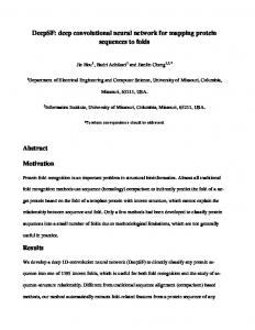
In this section, we present the modelling framework which is the backbone of fpgaConvNet (Fig. 1). A high-level overview of fpgaConvNet’s processing flow is as follows. As a first step, the Deep Learning specialist provides as inputs a high-level description of a ConvNet architecture together with information about the target FPGA-based platform by means of a domain-specific language that we designed. Next, the structure of the input ConvNet is captured by means of a DAG-based application model and information about the platform-specific resource constraints is extracted. The ConvNet DAG is then transformed into an SDF hardware intermediate representation that corresponds to a fully parallel hardware implementation. Each node of the SDFG corresponds to a hardware building block and the arcs indicate the interconnections between them. By applying a set of transformations on the SDF hardware model of the ConvNet, the design space is searched and this process yields a succession of hardware mappings of the ConvNet onto the particular FPGA-based platform. A. ConvNet Application Model A ConvNet is represented as a sequence of layers that form a directed acyclic graph (DAG) where each layer corresponds to a node. The set of layers with their connections and parameters are supplied by means of a high-level domainspecific description scheme, similar to the one used in [9], which is used to populate the semantic model of the ConvNet. Fig. 2 illustrates how a typical ConvNet would be described following our scheme. The high-level ConvNet description is passed through our DSL1 processor which parses the input script and populates the semantic model of the ConvNet in the form of a DAG by means of code generation. The ConvNet 1 Domain-Specific

Language

where ◦ N is the number of nonlinear units of the nonlinear layer. ◦ T is the type of nonlinear function to be applied, e.g. sigmoid, tanh or ReLU. •

Pooling Layer < P, S, N, T >

Fig. 1: Outline of fpgaConvNet’s Processing Flow

semantic model comprises a sequence of layers where each layer is instantiated with the supplied parameters.

where ◦ P is the pooling size which defines a (P × P ) pooling neighbourhood. ◦ S is the stride which defines the step between successive pooling windows. ◦ N is the number of pooling units in the pooling layer. ◦ T is the type of pooling operation to be applied, i.e. either max or average. B. FPGA-based Platform Model The FPGA-based platform model comprises a set of parameters describing the available on-chip resources and the off-chip memory characteristics. The resources of such an abstract FPGA-based platform are described using a resource set, R, which is the union of sets Rf pga and Rmem , and a vector, rscAvail. , storing the available amount for each of the elements in R: Rf pga = {DSP, LU T, Reg, BRAM } Rmem = {Bmem , Cmem } (1) R = Rf pga ∪ Rmem rscAvail. = [DSPAvail. , RegsAvail. , LU TAvail. , BRAMAvail. , Bmem , Cmem ]⊤

Fig. 2: ConvNet High-Level Description Each node in the ConvNet DAG represents a layer of the ConvNet architecture and is associated with a tuple of parameters. Currently, the following types of layers are supported, which are the ones that have been most commonly used in the ConvNet literature: •

Convolutional Layer < Kh , Kw , S, N > where ◦ Kh and Kw are the height and width of each filter in the convolutional layer, assuming kernels of dimensions (Kh × Kw ). ◦ S is the stride which defines the step between successive convolution windows. ◦ N is the number of filters that constitute the filter bank of the convolutional layer.

•

Nonlinear Layer < N, T >

(2)

where Bmem is the off-chip memory bandwidth and Cmem is the off-chip memory capacity. The off-chip memory bandwidth is modelled as: Bmem = ηBnom (3) where Bnom is the nominal bandwidth of the off-chip memory module and η ∈ [0, 1] is the efficiency factor which captures SDRAM and memory controller inefficiencies. C. Hardware Intermediate Representation The DAG model of the ConvNet is transformed into an SDF graph that represents a hardware mapping of the ConvNet. The structure of an SDFG can be represented in a compact form by the topology matrix, Γ. Each row of Γ corresponds to an arc and each column corresponds to a node in the SDFG. In conventional SDF, an element Γ(a, n) in the matrix specifies the rate of the data that flows from node n along arc a. In the case of data production, the rate of produced data is a positive integer while in the case of data consumption the rate of consumed data is a negative integer. In the proposed framework, we adopt the SDF paradigm [3] which is extended in two ways. First, the topology matrix is decomposed into the Hadamard product2 of three matrices that allows for a richer structural interpretation of its elements. 2 The Hadamard product, here denoted as ⊙, is defined as the elementwise multiplication between two matrices.

The first matrix is the channels matrix, denoted by C. Each element of C holds the width of a data stream, measured in words. Element C(a, n) holds the number of words that are present in parallel in outgoing or incoming arc a of node n. If the data are consumed by node n, the value is a negative integer, while if they are produced, it is a positive integer. The second matrix is the streams matrix, denoted by S. Each element of S indicates how many parallel streams are present on the particular arch on the side of the specified node. For instance, S(a, n) represents the number of streams, each of width C(a, n), that are present at arc a on the side of node n. All elements of S are non-negative integers. Finally, the third matrix is the rates matrix, denoted by R. Each element of R is a real number in the interval [0, 1] which specifies the normalised rate of data consumption or production by each node on each arc per cycle. 0 indicates no data flow and 1 shows a rate of 1 firing/cycle. A rate of 0.5 can be interpreted as 1 firing per 2 cycles or equivalently a firing period of 2 cycles. In addition, the rate of a node n is equivalent to the inverse of its initiation interval3 , IIn . The original topology matrix can be reconstructed by:

◦

Such a parametrisation allows us to capture different implementations for every hardware block, each with different performance-resource cost characteristics. In this way, fgpaConvNet is able to perform design space exploration by tuning the implementation of each block and moving around the design space. This process is further elaborated in Section V. At the same time, the Γ matrix ensures the functional correctness of each design point by propagating the data rates of each block. The tuples for the current set of available hardware building blocks that are used to map ConvNet layers to hardware are shown below. •

< param, sin , sout , cin , cout , rin , rout > where ◦ param is a set of configuration parameters, specific to each unit. ◦ sin and sout are the number of parallel streams at the input and output of the unit respectively. ◦ cin and cout are the number of words per stream at the input and output of the unit respectively. ◦ rin is the consumption rate, which is interpreted as the inverse of the initiation interval (II), in consumptions/cycle. 3 The initiation interval, here denoted as II, is defined as the number of cycles after which a new input can be fed to a pipelined unit.

1 > Sw

where ◦ N is the number of sliding window units. ◦ (Kh × Kw ) is the specified window size. ◦ Sh and Sw are the strides that determine the sliding step of the window along the feature map’s height and width respectively. A sliding window unit takes as input a stream of pixels and outputs a stream of (Kh × Kw ) windows with strides of Sh and Sw along the input feature map’s height and width respectively. •

Fork Unit < {Nin , N }, Nin , N × Nin , c, c, 1, 1 >

D. ConvNet Hardware Building Blocks To convert the ConvNet DAG into an SDF graph that corresponds to a hardware implementation, each node of the ConvNet DAG is to be mapped to a set of hardware building blocks that implement its functionality. The hardware building blocks are then interconnected to form the final SDF graph, with each building block occupying a column (i.e. a node of the SDFG) of Γ. In this way, the whole structure initially corresponds to a fully parallel mapping of the original ConvNet. In our prototype, the SDFG is used to generate synthesisable Vivado HLS code which is ready to be compiled by the Xilinx Vivado HLS tool. In the hardware intermediate representation, each building block is represented by a tuple of the following form:

Sliding Window Block < {N, Kh , Kw , Sh , Sw }, N, N, 1, Kh × Kw , 1,

Γ=S⊙C ⊙R

which can be interpreted as the overall data rate on all arcs and nodes of the graph. Our second extension of the SDF is that the final topology matrix is allowed to contain real values in its elements, because of the real-valued rates matrix. All four matrices are upper bidiagonal with non-zero elements only along the main diagonal and the diagonal above it.

rout is the production rate in productions/cycle.

where ◦ Nin is the number of input streams. ◦ N is the size of the fork operation. ◦ c is the number of words per stream. A fork unit takes as input a total of Nin streams with c words each and copies them to N × Nin output streams. •

Convolution and Pooling Banks < {N, Kh , Kw , uimp. }, N, N, Kh ×Kw , 1, uimp. , uimp. >

where ◦ N is the number of computing units in the bank. 1 ◦ uimp. ∈ [ Kh ×K , 1] is the folding factor of w the unit, normalised by the size of the input window, (Kh × Kw ). Each of the units in the bank performs an operation which reduces a window of size (Kh ×Kw ) to a single value. For convolution banks, the operation of each of the N units is a dot product between the input window and the corresponding weights. The input and output rates depend on the folding factor of the units, uimp. . If uimp. < 1, then the specified unit uses time-multiplexing of its MACC resources to compute a dot product. For pooling banks, we support two pooling operations: average pooling and max pooling. In the case of average pooling, dot product units are used with averaging kernels and therefore the average

pooling banks are configured similarly to convolution banks. On the other hand, in the case of max pooling banks, finding the maximum is performed with a 1 comparator and uimp. is equal to (Kh ×K with a w) single pixel being consumed per cycle. •

Nonlinear Bank ◦

◦

•

< {N, T }, N, N, 1, 1, 1, 1 >

N is the number of nonlinear units in the nonlinear bank. A nonlinear unit passes a stream of words through the specified nonlinear function. T is the type of nonlinear function to be applied, e.g. sigmoid, tanh or ReLU. Sigmoid and tanh are implemented using the piecewise linear approximation proposed in [10].

Memory I/O Unit < {N, W, Bnom , η}, N, N, W, W, η, η >

where ◦ N is the number of memory ports used. ◦ W is the width of the memory I/O subsystem data bus, in words. ◦ Bnom is the theoretical maximum bandwidth of the memory I/O subsystem. ◦ η is the normalised efficiency of the memory I/O subsystem and lies in the interval [0,1]. Therefore, in this model, the average bandwidth is estimated as Bmem. = ηBnom . V.

Our proposed alternative to this problem exploits the reconfigurability capabilities of FPGAs and suggests the partitioning of the ConvNet along its depth and the mapping of each partition to a different bitstream. A partition includes the splitting of the original SDFG into several subgraphs. Each subgraph is mapped onto a distinct hardware architecture. In this way, on-chip memory is used for data-reuse and intermediate results and the communication with the off-chip memory is kept to a minimum and limited to the subgraph’s required input and output streams. Following this process, we end up with one topology matrix and one hardware design per subgraph and consequently with one bitstream per subgraph. This approach requires the reconfiguration of the FPGA whenever data have to enter a different subgraph which adds a reconfiguration time overhead. By processing several input data streams in a pipelined manner or by having large input data streams, the reconfiguration time overhead is amortised. In this manner, we manage to introduce for the first time in the literature design points that require FPGA reconfiguration into the design space and expand the design capabilities. An illustration of this transformation is shown in Fig. 3.

Fig. 3: SDF Partitioning Example

S EARCHING THE D ESIGN S PACE

The exploration of the architectural design space is performed by applying a set of legal graph transformations. The legality of a transformation is defined as the functional equivalence of the graph before and after the transformation has been applied. We define three types of transformations: graph partitioning, coarse- and fine-grained folding. The first transformation includes the partitioning of the SDFG into subgraphs along the ConvNet depth by means of full FPGA reconfiguration. The second and third transformations include the local folding of the SDFG so that the building blocks are time-shared using time-multiplexing. These transformations provide a tunable trade-off between resource utilisation and performance. A. Graph Partitioning A fully parallel implementation of the ConvNet that follows the initial SDFG assumes that the on-chip memory as well as the compute resources of the target FPGA are able to accommodate it. However, in practice the on-chip memory requirements can scale rapidly with an increase either in the ConvNet’s depth in terms of number of layers, or in a layer’s width. The most common approach in the literature to deal with this issue is by means of a flexible and powerful hardware architecture that is time-shared across layers. Between two layers, data are streamed in and out of the device and are buffered in the off-chip memory. Although such a design typically yields a non-optimised execution of each particular layer, it enables the full evaluation of the ConvNet and exploits up to a degree the parallelism in each layer.

B. Coarse- and Fine-grained Folding A direct implementation of the original ConvNet SDFG, or of one of its subgraphs, would yield the maximum theoretical throughput. The high performance comes mainly as a result of two factors. The first factor is the fully unrolled execution of the coarse operations at each layer, such as the fully parallel execution of all convolutions in a filter bank, pooling operations in a pooling layer and nonlinearities in a nonlinear layer. A parametrisation over the unroll factor of a layer’s implementation offers a tunable design option. We define this as the coarse-grained folding of a layer. The second factor is the fully unrolled and pipelined implementation of the dot product operations inside convolutional and average pooling units. A fully parallel implementation of a dot product with inputs of size N would require N multipliers operating in parallel followed by an adder reduction tree with ⌈log2 N ⌉ stages and N − 1 adders. An additional adder can be included to combine the output of the dot product with other results. Such a fully unrolled implementation implies an initiation interval of 1 cycle and consequently a throughput of 1 dot product per cycle. On the other end of the spectrum, a dot product unit can be implemented as a single MACC unit with all the multiply-accumulate operations scheduled using timemultiplexing. In this case, the initiation interval is equal to the length of each input vector, i.e. N cycles, and hence the throughput is decreased to N1 dot products per cycle. Moreover, the resource utilisation is also decreased by approximately the same factor. A parametrisation over the unroll factor of dot

product units offers flexibility in the design options and another degree of freedom. We define this as the fine-grained folding of a layer. Algorithm 1 Coarse-grained Folding Transformation 1: - Inputs: matrix Γ Index i of the layer to be folded Nominal size Nnom of the layer to be folded Folding factor, f ∈ [ N 1 , 1] nom 2: - Initialise folding vector, fcoarse ∈ R#colsΓ : fcoarse = 1 3: - fcoarse (i) = f 4: - Form the folding matrix, F = diag(fcoarse ) 5: - Apply the coarse-grained folding, S ′ = ⌈S · F ⌉ 6: - Form the folded topology matrix, Γ′ = S ′ ⊙ C ⊙ R Note: ⌈·⌉ is defined as the element-by-element ceiling operator

Algorithm 2 Fine-grained Folding Transformation 1: - Inputs: matrix Γ Index i of the layer to be folded Kernel size K or pooling size P Folding factor, f ∈ [ K12 , 1] or [ P12 , 1] 2: - Initialise folding vector, ff ine ∈ R#colsΓ : ff ine = 1 3: - ff ine (i) = f 4: - Form the folding matrix, F = diag(ff ine ) 5: - Apply the coarse-grained folding, R′ = ⌈R · F ⌉ 6: - Apply the fine-grained folding, Γ′ = S ⊙ ⌈C ⊙ R′ ⌉ Note: ⌈·⌉ is defined as the element-by-element ceiling operator

The control over the degree of exploitation of coarseand fine-grained parallelism corresponds to two degrees of freedom that allows us to tune the performance-resource tradeoff and explore the design space. With reference to the building block models presented in Section IV, a convolutional, pooling or nonlinear layer of nominal size Nnom is mapped to the corresponding bank block. The coarse-grained folding of operators is controlled by parameter N of the bank model, which corresponds to the actual number of units that will perform the Nnom operations. The range of N is [1, Nnom ] which corresponds to a coarse folding factor in the range 1 [ Nnom , 1] with 1 mapping to a fully unrolled implementation 1 to a single unit with time-multiplexing. Similarly, and Nnom the fine folding factor of convolutional and pooling units is 1 , 1] where 1 corresponds to set by parameter uimp. ∈ [ Kh ×K w 1 maps to a fully a fully unrolled implementation and Kh ×K w folded implementation. Our SDF modelling approach allows us to express these transformations algebraically. In this way, the coarse- and finegrained transformations are applied directly to the topology matrix Γ by means of a folding vector as described by algorithms (1) and (2) respectively. The implications of our approach are that we can explore the design space faster by using algebraic operations on our SDF model without the need to synthesise or implement various different hardware designs to get an estimate of their performance-resources characteristics and at the same time ensure functional correctness. Moreover, assigning values to the parameters of the transformations can be formulated as a formal optimisation problem. C. Performance Model Given an SDF representation of a hardware mapping, the columns of the topology matrix Γ give the throughput of each hardware block in consumptions/cycle at the input and

productions/cycle at the output, after the depth of the unit’s pipeline has been filled. The amount of work, Wi , carried out by the ith hardware block is equivalent to the total number of pixels to be consumed by this block and can be expressed as shown below. Wi = Fiin · Piin where Fiin is the number of feature maps at the input of the ith hardware block and Piin is the number of pixels per feature map. To propagate the work along the whole SDFG, we introduce the feature maps matrix, Fmap , and the pixels matrix, P , and form the work matrix, W as shown below. W = Fmap ⊙ P To find the initiation interval of each hardware block, it suffices to divide W by Γ, element by element. II = W ⊘ Γ

where II is the initiation interval matrix. Each element of II gives the number of cycles required by each hardware block along the processing pipeline to consume its workload. The hardware block with the longest initiation interval determines the initiation interval of the whole SDFG and is given by the maximum element of II, denoted by II max . Overall, the execution time of all the computations needed for a total of M images can be estimated by Eq. (4).

1 (4) · II max · (M − 1) clock rate where D is the pipeline depth of the SDFG divided by the operating clock rate. In the case where an SDFG is partitioned into subgraphs that will be executed sequentially after FPGA reconfiguration, the overall execution time can be estimated by summing the execution times of all the subgraphs. For this case, we extend the notation of Eq. (4) with ti to denote the execution time of the ith partition. Whenever reconfiguration takes place between the execution of consecutive subgraphs, the reconfiguration time for the ith reconfiguration, ti,reconf ig. , has to be included. Eq. (5) gives the total execution time for NP partitions. NP N! P −1 ! ttotal (M, NP , Γ) = ti (M, Γi ) + ti,reconf ig. (5) t(M, Γ) = D +

i=1

i=1

where Γi is the topology matrix of the ith partition. In our approach, we assume full reconfiguration of the FPGA device and hence ti,reconf ig. can be considered constant for all i. In this case, Eq. (5) can be simplified as: ttotal (M, NP , Γ) =

NP ! i=1

ti (M, Γi ) + (NP − 1) · treconf ig. (6)

From Eq. (6), we observe that the reconfiguration overhead is independent of the number of images that are processed. Therefore, by either increasing the total number of input images or their sizes, the first term dominates the execution time and the cost of reconfiguration is amortised. In practice, the value of M is limited by the capacity, Cmem , of the available off-chip memory. Finally, the throughput of an implementation of a particular ConvNet in GOp/s which requires WConvN et GOp/frame can be estimated as in Eq. (7). WConvN et T (M, NP , Γ) = (7) ttotal (M, NP , Γ)/M

D. Optimisation Given the defined transformations, we pose the following combinatorial optimisation problem: max T (Γ), s.t. rsc(Γ) ≤ rscAvail. (11) Γ

where T and rsc return the throughput in GOp/s and resource consumption of the current implementation and rscAvail. is the vector with the available resources on the target platform. The optimisation considers the partitioning, coarse- and finegrained folding transformations and aims to find partition points and coarse- and fine-grained folding factors that maximise the throughput of a ConvNet hardware mapping onto the target FPGA platform. The partitioning transformation can be cast to a search problem, where we aim to maximise the overall performance by selecting adequate partition points. For a ConvNet with NL layers, there are NL − 1 candidate partition points with a minimum of one partition and a maximum of NL partitions. The total number of design points that correspond to different partitionings is 2NL −1 . In our optimisation framework, we form a partitioning vector p ∈ {0, 1}NL −1 where a value of 1 for the ith element indicates that the SDFG will be partitioned at the ith layer. Coarse-grained folding can be applied to any type of layer. Therefore, the coarse-grained folding vector, fcoarse has NL elements, where each element has a different range as explained in Section V. Fine-grained folding can be applied on convolutional and average pooling layers and the range of candidate values for each folding factor depends on the window size at each layer. Similarly to the coarse-grained folding case, the fine-grained folding vector, ff ine , has NL elements. The overall number of design points to be explored given all three transformations can be found as shown below: NL NL " " DesignP ointsT otal = 2NL −1 · Ncoarse,i · Nf ine,i i=1

i=1

where Ncoarse,i and Nf ine,i are the number of possible coarseand fine-grained folding factors for the ith layer respectively. With an increase in either the depth or the width of a ConvNet’s layers, a brute-force enumeration approach quickly becomes a computationally intractable problem. Therefore, a heuristic method should be used instead to obtain an approximate solution in the non-convex design space. Currently, we have selected Simulated Annealing [11] as our heuristic method. VI.

E VALUATION

The target platform is Zynq-7000 XC7Z020 FPGA with an operating frequency of 100 MHz. Xilinx Vivado HLS and Vivado Design Suite (v15.4) were used and all hardware implementations were run on Avnet’s ZedBoard. fpgaConvNet provides support for fixed-point as well as single- and doubleprecision floating-point representation. In the evaluation phase, Q8.8 fixed-point representation was used which is also used in the FPGA works that we compare with and has been extensively tested in the literature to give similar results to neural networks implemented in 32-bit floating-point [6]. A. Benchmarks For the evaluation of fpgaConvNet, we selected a set of six ConvNet benchmarks. These include three well-known

TABLE I: FPGA Resource Utilisation for each Benchmark LUT (Total Available: 53200) Utilisations 34.78% 16.11% 26.30% 12.23% 59.00% 10.16% 11.20% 16.19% 30.24% 29.74% 14.00% 20.96% 57.86% 23.82% 11.70%

Flip-Flops (Total Available: 106400) Utilisations 22.10% 10.37% 21.53% 7.12% 52.68% 5.83% 6.90% 10.35% 21.39% 21.07% 7.94% 12.41% 39.27% 16.96% 7.14%

DSP Slices (Total Available: 220) Utilisations 24.09% 1.82% 1.82% 0% 3.63% 0% 0% 1.82% 4.09% 22.72% 0% 0% 65.45% 12.27% 0%

BRAM (Total Available: 630KB) Utilisations 3.21% 3.21% 6.78% 3.21% 4.64% 3.21% 3.21% 6.07% 8.57% 6.78% 3.21% 3.21% 6.07% 4.28% 3.21%

P3

48.46%

35.58%

7.27%

6.07%

P4 P5 P1

12.09% 42.23% 35.20%

7.32% 30.46% 25.57%

0% 65.45% 85.45%

3.21% 6.43% 5.00%

P2

66.64%

49.44%

94.54%

6.07%

P3

81.23%

34.72%

35.45%

8.57%

Benchmarks Name CFF [12] LeNet-5 [13]

MPCNN [14]

CNP [4]

Sign Recognition [7]

Partition P1 P1 P2 P3 P1 P2 P3 P4 P1 P2 P3 P4 P5 P1 P2

Scene Labelling [15]

TABLE II: Predicted vs. Measured Performance Benchmarks CFF [12] LeNet-5 [13] MPCNN [14] CNP [4] Sign Recognition [7] Scene Labelling [15]

Predicted Performance 10.14 GOp/s 0.49 GOp/s 0.79 GOp/s 3.63 GOp/s 6.36 GOp/s 12.95 GOp/s

Measured Performance 9.10 GOp/s 0.48 GOp/s 0.74 GOp/s 3.53 GOp/s 6.03 GOp/s 12.73 GOp/s

Error -11.76% -2.08% -6.04% -2.83% -5.47% -1.73%

ConvNets for computer vision applications with different computational loads, namely the Convolutional Face Finder (CFF) [12], LeNet-5 [13] and MPCNN [14]. We also implemented two ConvNets from existing FPGA works [4][7] for scene labelling and sign recognition which we denote CNP and Sign Recognition respectively, and one ConvNet for scene labelling from an embedded GPU work [15]. B. Predictive Accuracy To evaluate the quality of our model, we implemented all six benchmarks and compared the predicted and the achieved performance. We should note that for this task, the hardware mappings for CFF, LeNet-5 and MPCNN are not the best ones given by our framework, but only random instances without using Simulated Annealing. For the CNP, Sign Recognition and Scene Labelling ConvNets, we implemented the best designs as selected by fpgaConvNet. Table II shows the predicted versus the measured performance in GOp/s for each of the benchmark applications together with the average errors in the prediction. The model’s predictions are fairly close to the measurements on the Zynq platform for all ConvNets, with the predictions giving slightly optimistic throughputs. This is due to the fact that our model assumes that the depth of each SDF pipeline has been filled and hence does not include its overhead in its predictions. Moreover, additional I/O delays, reconfiguration time variations and software overhead also contribute to the small error of the predictions. The average error does not exceed 12% and manages to be as low as 1.73%.

−4

Performance Density (GOp/s/Slice)

6

x 10

Existing Work GOp/s/Slice fpgaConvNet GOp/s/Slice fpgaConvNet Non−Amortised GOp/s/Slice

5 4 3 2 1 0

CNP [4]

Sign Recognition [7]

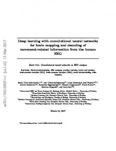
Fig. 4: Performance Density Comparison with existing works C. Performance Comparison To evaluate the quality in terms of performance of the design point that is selected by our framework, we compare fpgaConvNet with the FPGA works of [4] and [7] and the embedded GPU work of [15]. Fig. 4 shows the the performance density with respect to slices. In terms of performance density, fpgaConvNet outperforms CNP by 1.62× and is slightly above the performance density of [7]. In terms of raw performance, when the overhead due to the FPGA reconfiguration is amortised, fpgaConvNet reaches 90.75% of CNP’s throughput and 35% of the sign recognition ConvNet’s performance in [7]. An important factor to take into account is that CNP runs at 1.5× higher clock frequency while the device used in [7] has 3.5× more DSPs compared to our platform and their design runs at 1.5× higher clock frequency. Consequently, fpgaConvNet manages to reach and in some cases outperform the two FPGA designs in terms of performance density despite running at a lower clock frequency and having fewer DSPs. All existing FPGA works do not include full FPGA reconfiguration. To investigate the effect of FPGA reconfiguration on fpgaConvNet’s performance, we also display in red the throughput when the reconfiguration time is not amortised due to the limited number of images. In this case, only 254 images are used on each ConvNet to compensate for the reconfiguration overhead and hence the achieved performance is severely degraded. As a result, by allowing reconfiguration as one of the transformations explored by our framework, non-latency critical applications should be targeted. Nevertheless, in applications that handle large size images, a small number of images is required to fully amortise the reconfiguration overhead. In these cases, large images increase the computation-to-reconfiguration time ratio, but at the expense of higher on-chip memory requirements for line buffering inside sliding window units. Finally, we compared the fpgaConvNet’s performance with the embedded GPU work presented in [15] for the same scene labelling ConvNet. As shown in table III, our framework reaches 16.75% of the Tegra K1’s sustained performance as reported in [15], clocked at 1/8 of the frequency and overpasses its performance efficiency in GOp/s/W by 1.05×. VII.

TABLE III: Performance Comparison with embedded GPU Implementation

Device

fgpaConvNet Scene Labelling [15]

Zynq-7000 XC7Z020 Tegra K1

Performance per Power 7.27 GOp/s/W 6.91 GOp/s/W

of algebraic operations and enables the formulation of a ConvNet’s hardware mapping as an optimisation problem. Experimental evaluation shows that fpgaConvNet gives fairly accurate performance predictions and achieves improvements in performance density and performance efficiency over existing FPGA and embedded GPU works. Potential future work includes an investigation of how we can maximise the performance of fpgaConvNet by introducing additional graph transformations as well as its integration with TensorFlow [16]. R EFERENCES [1] [2]

[3] [4] [5] [6] [7] [8]

[9] [10]

[11] [12]

[13] [14]

C ONCLUSION

This paper presents fpgaConvNet, a framework for mapping Convolutional Neural Networks on FPGAs. The proposed methodology captures ConvNets by means of an analytical SDF model. We present a set of graph transformations and introduce for the first time FPGA reconfiguration as a design option for ConvNet FPGA implementations. This approach allows the fast exploration of the design space by means

Sustained Performance 12.73 GOp/s 76.00 GOp/s

[15] [16]

Y. Bengio, “Learning Deep Architectures for AI,” Found. Trends Mach. Learn., vol. 2, no. 1, pp. 1–127, Jan. 2009. A. Coates, B. Huval, T. Wang, D. J. Wu, B. C. Catanzaro, and A. Y. Ng, “Deep learning with COTS HPC systems,” in Proceedings of the 30th International Conference on Machine Learning, ICML 2013, Atlanta, GA, USA, 16-21 June 2013, 2013, pp. 1337–1345. E. A. Lee and et al., “Synchronous Data Flow,” 1987. C. Farabet, C. Poulet, J. Y. Han, and Y. Lecun, “CNP: An FPGA-Based Processor for Convolutional Networks,” in International Conference on Field Programmable Logic and Applications. IEEE, 2009. C. Farabet, B. Martini, B. Corda, P. Akselrod, E. Culurciello, and Y. LeCun, “Neuflow: A Runtime Reconfigurable Dataflow Processor for Vision,” in CVPRW. IEEE, 2011, p. 109116. V. Gokhale, J. Jin, A. Dundar, B. Martini, and E. Culurciello, “A 240 gops/s mobile coprocessor for deep neural networks,” in CVPRW. IEEE, June 2014, pp. 696–701. M. Peemen, A. A. A. Setio, B. Mesman, and H. Corporaal, “Memorycentric accelerator design for Convolutional Neural Networks,” in ICCD. IEEE Computer Society, 2013, pp. 13–19. C. Zhang, P. Li, G. Sun, Y. Guan, B. Xiao, and J. Cong, “Optimizing FPGA-based Accelerator Design for Deep Convolutional Neural Networks,” in Proceedings of the 2015 ACM/SIGDA International Symposium on Field-Programmable Gate Arrays, ser. FPGA ’15. New York, NY, USA: ACM, 2015, pp. 161–170. Y. Jia, E. Shelhamer, J. Donahue, S. Karayev, J. Long, R. Girshick, S. Guadarrama, and T. Darrell, “Caffe: Convolutional Architecture for Fast Feature Embedding,” arXiv preprint arXiv:1408.5093, 2014. H. Amin, K. Curtis, and B. Hayes-Gill, “Piecewise Linear Approximation applied to Nonlinear Function of a Neural Network,” Circuits, Devices and Systems, IEE Proceedings -, vol. 144, no. 6, pp. 313–317, Dec 1997. C. R. Reeves, Ed., Modern Heuristic Techniques for Combinatorial Problems. New York, NY, USA: John Wiley & Sons, Inc., 1993. C. Garcia and M. Delakis, “Convolutional Face Finder: a Neural Architecture for Fast and Robust Face Detection,” Pattern Analysis and Machine Intelligence, IEEE Transactions on, vol. 26, no. 11, pp. 1408– 1423, Nov 2004. Y. Lecun, L. Bottou, Y. Bengio, and P. Haffner, “Gradient-Based Learning Applied to Document Recognition,” in Proceedings of the IEEE, 1998, pp. 2278–2324. J. Nagi, F. Ducatelle, G. Di Caro, D. Ciresan, U. Meier, A. Giusti, F. Nagi, J. Schmidhuber, and L. Gambardella, “Max-Pooling Convolutional Neural Networks for Vision-based Hand Gesture Recognition,” in Signal and Image Processing Applications (ICSIPA), 2011 IEEE International Conference on, Nov 2011, pp. 342–347. L. Cavigelli, M. Magno, and L. Benini, “Accelerating real-time embedded scene labeling with convolutional networks,” in Design Automation Conference (DAC), 2015 52nd ACM/EDAC/IEEE, June 2015, pp. 1–6. M. Abadi et al., “TensorFlow: Large-Scale Machine Learning on Heterogeneous Systems,” 2015, software available from tensorflow.org. [Online]. Available: http://tensorflow.org/