Fractional Wavelet Filter for Camera Sensor Node with external Flash and extremely little RAM Stephan Rein
[email protected]
Stephan Lehmann
[email protected]
Clemens Gühmann
[email protected]
Wavelet Application Group Department of Energy and Automation Technology Chair of Electronic Measurement and Diagnostic Technology Technische Universität Berlin
ABSTRACT
allows coding algorithms to achieve superior compression gains among current picture compression techniques. A This paper introduces the fractional wavelet filter as a techstandard coding technique is the SPIHT algorithm [9] that nique to compute fractional values of each wavelet subband, especially outperforms other techniques for high compresthus allowing a low-cost camera sensor node with less than sion rates while being conceptually fairly simple. However, 2 kByte RAM to perform a multi-level 9/7 picture wavelet as the wavelet transform itself is a memory intensive protransform. The picture dimension can be 256x256 using cedure, wavelet based compression has hardly arrived on fixed-point arithmetic and 128x128 using floating-point ariththe low energy consuming micro-controllers that drive low metic. The technique is applied to a typical 16 Bit sensor cost sensor nodes. Thus the design of low-memory wavelet node architecture with external flash memory, which allows transform schemes is still a current research activity, see secto line-wisely read and write picture data. tion 1.1. This paper addresses this problem by introducing a wavelet filter system - that is, the fractional wavelet filCategories and Subject Descriptors ter, for the Daubechies 9/7 wavelet (also called the FBIWavelet), which reads and writes the picture data rowI.4.10 [Computing Methodologies]: Image Processing and Computer Vision—Image Representation; B.3.2 [Hardware]: wisely and roughly allocates 1.2 kBytes for a fixed-point wavelet transform with the picture dimension N=256. We Memory Structures—Design Styles do not consider the conceptually less complex 5/3 wavelet transform that works with less coefficients or the integer General Terms wavelet transform, as these generally give lower compresAlgorithms, Performance, Measurement sion gains. The fractional filter is applied and evaluated on an own sensor node architecture called Spisa (see http://www.mdt. Keywords tu-berlin.de/research/wavelets) or OpenSensor [8]. It Fractional wavelet filter, Camera sensor node, Flash memory uses the Microchip dsPIC30F4013, i.e., a 16 Bit digital signal controller with 2 kByte RAM, the camera module C3287640 with an universal asynchronous receiver/transmitter 1. INTRODUCTION (UART) interface (available at http://www.comedia.com. Camera sensor nodes are small wireless devices that gather, hk), and an external 64 MByte secure digital (SD) card as process and transfer environmental pictures. These devices a flash memory, connected to the controller through a serial can be stationary or mounted on moving objects. A possiperipheral interface (SPI) bus. The data of the SD-card is ble application for a camera sensor network may be remote accessed through an own filesystem [10]. Camera and SDassistance for moving vehicles concerning localization and card both can be connected to any controller with UART computer-assisted maintenance. and SPI ports. The system is designed to capture still imAs the bandwidth is very limited in wireless sensor netages. works, data compression techniques are inevitable when large The paper is organized as follows. In the next subsecamounts of data, e.g., pictures, have to be transferred. The tion, related literature is reviewed. In section 2, the main wavelet transform is an established decorrelating tool that principle of the picture wavelet transform and its implementation is outlined. In section 3, the fractional filter for the wavelet transform is detailed. We have implemented two forward transforms, one using floating-point numbers for high Permission to make digital or hard copies of all or part of this work for precision and another transform using fixed-point numbers personal or classroom use is granted without fee provided that copies are that needs less memory while being computationally more not made or distributed for profit or commercial advantage and that copies bear this notice and the full citation on the first page. To copy otherwise, to suitable for a 16 Bit controller. In section 4, the two implerepublish, to post on servers or to redistribute to lists, requires prior specific mentations for the fractional filter are evaluated on a 16 Bit permission and/or a fee. signal controller sensor node with two kByte RAM concernMobiMedia ’08, July 7-9, 2008, Oulu, Finland ing picture quality, flash memory access and computation Copyright 2008 ACM ISBN 978-963-9799-25-7/08/07 ...$5.00.
times. In the last section we conclude the paper and describe our future work.
1.1 Related Work One major difficulty in applying the discrete two- dimensional wavelet transform to a platform with scarce resources is the need for large memory. Implementations on a personal computer (PC) generally keep the whole source and/or destination picture in memory, where horizontal and vertical filters are applied separately. As this is generally not possible on a resource-limited platform, the recent literature addresses the memory-efficient implementation of the wavelet transform. A very large part of the literature concerns the implementation of the wavelet transform on field programmable gate arrays (FPGA), see for instance [11, 3, 1, 4]. The FPGA-platforms are generally designed for one special purpose and are not an appropriate candidate for a sensor node that has to perform many tasks concerning communication and analysis of the surrounding area, see [5, 8] for details. This work is different from the literature on FPGAs in that it considers the 9/7 picture wavelet transform for a micro- or a signal-controller with very little RAM. Such a solution can easily be integrated in current sensor network platforms and offers much flexibility. Costs and programming efforts are limited as the extension only concerns a standard SD-card, a camera module, and a software module for the transform. The most related work to this paper is given in [2], where a line-based version of the wavelet transform is given. The authors describe a system of buffers where only a small subset of the coefficients has to be stored thus tremendously reducing the memory requirements compared to the traditional approach. A very efficient implementation of the line-based transform using the lifting scheme and improved communication between the buffers is detailed in [6], where the authors use a PC-based C++ implementation for demonstration. However, in the context of our requirements it is not applicable to a sensor node with extremely little RAM as it uses in ideal case 26 kByte RAM for a six-level transform of an 512x512 picture, whereas the approach given in this paper would only require roughly 5 kByte using the floating-point scheme. We could not find any paper where the 9/7 picture wavelet transform is implemented on a low-cost 16 Bit signal-/micro-controller.
2.
WAVELET TRANSFORM
A tutorial on the picture wavelet transform and its features is given in [12]. We here just outline how the wavelet transform can be computed with filter operations while we start with one dimension to explain the basics for the picture transform. In the following subsections the fractional wavelet filter is detailed using floating-point and fixed-point numbers.
2.1 Wavelet Filtering A one-dimensional discrete wavelet transform can be performed by low- and highpass filtering of an input signal with the dimension N , which can be a single line of a picture. The two resulting signals are then sampled down - that is, each second value is discarded, and then form the approximations and details, which are two sets of N/2 wavelet coefficients. In this work the Daubechies biorthogonal 9/7 filter is employed, which is part of the JPEG2000 standard and the basis for many wavelet compression algorithms, including
lowpass real Q15 0.852699 27941 0.377403 12367 -0.110624 -3625 -0.023849 -781 0.037828 1240
index 0 ±1 ±2 ±3 ±4
highpass real Q15 0.788486 25837 -0.418092 -13700 -0.040689 -1333 0.064539 2115 0 0
Table 1: 9/7 Analysis wavelet filter coefficients in real and Q15 data format. the embedded zerotree (EZW) or the set partitioning in hierarchal trees (SPIHT) algorithm [12]. The approximations L(i) can be computed with L(i) =
4 X
linepic (i + j) · Al(j),
i = 0 . . . N − 1 (1)
j=−4
and the details H(i) with H(i) =
3 X
linepic (index + i) · Ah(j),
i = 0 . . . N − 1,
j=−3
(2) where Al(j) and Ah(j) denote the filter coefficients given in table 1, respectively. Note that the sample down operation can be incorporated by only computing the required coefficients, thereby avoiding useless computation. At the signal boundaries, we perform a symmetrical extension to avoid border effects, e.g., a signal s(i), i = 0 . . . N − 1 is extended for the highpass filter as follows: sext = s(3)s(2)s(1)s(0)s(1) . . . s(N −1)s(N −2)s(N −3)s(N − 4) The filter is slided over the signal in such a way that the center of the filter is located upside the i th signal value s(i), e.g., for i = 1: Ah(-3) s(2)
Ah(-2) s(1)
Ah(-1) s(0)
Ah(0) s(1)
Ah(1) s(2)
Ah(2) s(3)
Ah(3) s(4)
For the lowpass filter the center of the filter slides over the even values i = 0, 2, . . . , N − 1, for the highpass it moves over the odd values i = 1, 3, 5, . . . N . A one-level picture wavelet transform can be computed by first performing a one-dimensional transform for each line and then repeat this operation for all the columns of the result - that is, apply the low- and the highpass in vertical direction. The horizontal transform results into two matrices with N rows and N/2 columns, which we denote by L and H for the approximations and details, respectively. The second operation leads to four square matrices of the dimension N/2 denoted by LL, HL, LH, HH, which are the so-called subbands. The two operations can be repeated on the LL subband to get the higher level subbands, e.g., HL2 refers to the second level HL subband that is computed by first horizontally filtering LL1 and then vertically filtering the result. An example of a two-level wavelet transform is given in figure 1.
3. FRACTIONAL WAVELET FILTER In this section the fractional wavelet filter - that is, a computational scheme to compute the picture wavelet transform with very little RAM memory, is explained. The data on the SD-card can only be accessed in blocks of 512 Bytes, thus a sample-wise access as easily executed with RAM memory
LL2
HL2
HL1 SD−card pic
destination LL
vertical filter area
LH1
HL
LH
HH
HH1
Figure 1: An example of a 2-level picture wavelet transform. Each one-level transform results into four subbands denoted by LL, LH, HL, HH. The contrast of each subband was adjusted to fill the entire intensity range.
on PCs is here not feasible. Even if it is possible to access a smaller number of samples of a block, the read/write time would significantly slow down the algorithm, as the time to load a few samples is the same as for a complete block. The fractional filter has to take this restriction into account. For the first level, the algorithm reads the picture samples line by line from the SD-card while it writes the subbands line-wisely to a different destination on the SD-card. Two single lines of the LL/HL subbands and two lines of the LH/HH subbands build a destination line, respectively. For the next level the LL subband contains the input data. Note that the input samples for the the first level are of the type unsigned char (8 Bit), whereas the input for the higher level are either of type float (floating point filter) or INT16 (fixedpoint filter) format. The filter does not work in place and for each level a new destination matrix is allocated on the SD-card. However, as the SD-card has plenty of memory, it does not affect the sensor’s resources. This also allows to reconstruct the picture from any level (and not necessarily from the highest level, as it would be necessary for a transform illustrated in figure 1). The scheme is illustrated in figure 2.
3.1 Floating-Point Filter The floating point wavelet filter computes the wavelet transform with a high precision, as it uses 32 Bit floating point variables for the wavelet and filter coefficients as well as for the intermediate operations. Thus the pictures can be reconstructed without loss of information. The wavelet filter uses three buffers of the dimension N - one for the current input line and two buffers for two destination lines each of them building a row of the LL/HL subbands and a row of the LH/HH subbands. The filter computes the horizontal wavelet coefficients on the fly, while it computes a set of fractions (here we denote fractions as a part of a sum) of each subband destination line. Let ll(i, j, k), lh(i, j, k), hl(i, j, k), and hh(i, j, k) denote the fractional subband wavelet coefficients, where i = 0, 2, 4, . . . N/2 − 1 and j = −4 · · · + 4 assign the current input line as i ∗ 2 + j. k = 0 . . . N/2 − 1 denotes
read line
FLOAT/INT16 FLOAT/INT16 UCHAR
current input row
LL
update FLOAT/INT16 LH
horizontal filter
HL
HH
Al(j)/Ah(j)
Figure 2: Proposed system for the picture wavelet transform. The horizontal wavelet coefficients are computed on the fly and employed to compute the fractional wavelet coefficients that update the subbands. For each wavelet level, a different destination object is written to the SD-card. Thus the picture can be reconstructed from any level. the horizontal coefficient index. The fractional coefficients are defined as follows: ll(i, j, k) = Al(j)
4 X
pic(i ∗ N + k + l) · Al(l)
(3)
3 X
pic(i ∗ N + k + l) · Al(l)
(4)
4 X
pic(i ∗ N + k + l) · Ah(l)
(5)
3 X
pic(i ∗ N + k + l) · Ah(l)
(6)
l=−4
lh(i, j, k) = Ah(j)
l=−3
hl(i, j, k) = Al(j)
l=−4
hh(i, j, k) = Ah(j)
l=−3
The final coefficients are computed by update operations and thus first have to be initialized: LL(i, k) = LH(i, k) = HL(i, k) = HH(i, k) = 0 |∀i,k . For j = −4 . . . 4, the update operations are then given by LL(i, k)+ = ll(i, j, k) HL(i, k)+ = hl(i, j, k)
LH(i, k)+ = lh(i, j, k) HH(i, k)+ = hh(i, j, k)
(7) (8)
The special requirement for the fractional filter is that j stays constant for updating all subband rows. The process of updating the destination lines is repeated until the final
subband coefficients have been estimated. The pseudo-code of this procedure uses the horizontal filter functions filtL and filtH. The low- and highpass filter coefficients from table 1 are accessed through al(j) and ah(j), where j denotes the filter index. The floating-point code for the first level is given as follows: FLOAT LL HL [N ] ; FLOAT LH HH [N ] ; UINT8 l i n e p i c [N ] ; / / c u r r e n t row INT8 i ; / / c u r r e n t row i n d e x INT8 j ; / / v e r t i c a l f i l t e r i n d e x INT8 k ; / / h o r i z o n t a l d e s t i n a t i o n i n d e x f o r ( i=N/2 −1; i >=0; i −−){ // i n i t th e two d e s t i n a t i o n b u f f e r s : UINT8 b ; f o r ( b=0;b