where x = s(f) corresponds to a free boundary, S~ (resp. S+) is an open subset of. I x (0, oo) in which xs(0), d{ and μf(i = 1, 2) are positive constants,.
HIROSHIMA MATH. J. 17 (1987), 241-280
Free boundary problems for some reaction-diffusion equations Masayasu MIMURA, Yoshio YAMADA and Shoji YOTSUTANI (Received September 17, 1986)
§ 1.
Introduction
The present paper deals with a free boundary problem which models regional partition phenomena arising in population biology. Our problem is to look for a family of functions {w(x, 0> s(t)} ((x, i) e [0, 1] x [0, oo)) which satisfy ut = d,uxx + uf(u)
in S-,
(1.1)
ut = d2uxx + ug(ύ)
in S+,
(1.2)
!i(0,ί) = 0
for
f e(0, oo),
(1.3)
ιι(l, 0 = 0
for
t E (0,oo),
(1.4)
u(s(t), 0 = 0
for
ί e (0, oo) ,
(1.5)
ti-O* 0 + μ2uMt) + 0, 0 for
w(x, 0) = φ(x)
ίe(0, oo) where
for
0 < s(t) < 1,
x e / = (0, 1) ,
5(0) = /,
(1.6) (1.7) (1.8)
where x = s(f) corresponds to a free boundary, S~ (resp. S+) is an open subset of I x (0, oo) in which xs(0), d{ and μ f (i = 1, 2) are positive constants, 5(0 denotes (d/dt)s(t) and wx(s(0~0, 0 (resp. wx(s(0 + 0, 0) means the limit of w(x, 0 at x = s(t) from the left (resp. right). For the derivation of the free boundary problem (1. !)-(!. 8), we refer the reader to [8]. In (1.1) and (1.2), /and g are assumed to possess the following properties: (A.I) / is locally Lipschitz continuous on [0, oo) and satisfies /(1) = 0 and /(w)^Oon [1, oo). (A.2) g is locally Lipschitz continuous on (—00, 0] and satisfies #(1) = 0 and 0(w)= 0on(-oo, -1]. On the initial data {φ, 1} we put the following conditions: (A.3) (A.4)
0^/ = 1. φeH^I) satisfies φ(ϊ) = 0 and (/-x)φ(x)^0 for x e / = [0, 1].
242
Masayasu MIMURA, Yoshio YAMADA and Shoji YOTSUTANI
Some related results for the problem (1.1)-(1.8), which is denoted by (P), can be found in our previous papers [8, 9] where we have studied the global existence, uniqueness, regularity and asymptotic behavior of solutions {u, s} with non-homogeneous Dirichlet boundary conditions (0, t) = m^ > 0 and w(l, t) = - w 2 < 0
M
for ίe(0, oo).
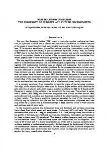
Owing to the non-homogeneity, it is proved there that the free boundary x = s(t) never touches the fixed boundaries x = 0, 1. However, when homogeneous Dirichlet boundary conditions are imposed, there is also the possibility that the free boundary hits one of the fixed ends x = 0, 1 in a finite time; that is, one phase disappears in a finite time. See Fig. 1, where some numerical experiments exhibit the disapperance of one phase in appropriate conditions. This is a very interesting phenomenon to discuss, though the analysis will be complicate.
ix = s(t)
Fig. 1 (1A and IB). dl=d2=μl=μ2 = l, a. sin πx/l
Ϊ
f(u)=g(-u)=a(l-u), for
-βsmπ(x-l)/(l-l)
for
Now the purpose of this paper is to study the global existence, uniqueness, regularity and asymptotic properties of solutions for (P) in the homogeneous case. The essential points of our analysis are almost the same as those developed by the authors in [8, 9]. Moreover, we intend to derive some conditions which guarantee the disappearance of one phase. In §2, we construct a solution {w, s} and derive its regularity properties over a time interval where the free boundary is distant from the fixed boundary. It will
Free boundary problems
243
be shown in §3 that, if the free boundary hits the fixed boundary at a finite time t= T*9 the free boundary stays there after T*. So we can continue to solve u as a solution of the usual initial boundary value problem for ί^ T* (cf. Fig. IB). The global existence result is stated in this section (Theorem 3.1). In §4, we give two comparison theorems for (P), which will help us to investigate the asymptotic properties of solutions for (P). In §5, we show some results about the dependence of {M, s} on the initial data {φ, I}. These results will be used for studying the ω-limit set corresponding to the solution orbit for (P). Complete information on the ω-limit set is stated in §6 (Theorem 6.2). Especially, it is shown that any element of the ω-limit set satisfies the stationary problem associated with (P). So the analysis of the stationary problem becomes very important. It is carried out in §7 by putting some restrictions on the forms of /and g. In §8, stability or instability of each stationary solution is investigated with use of the comparison technique. Moreover, we give some sufficient conditions for the disappearance of one phase in a finite time. Finally, §9 is devoted to the study of bifurcation phenomena appearing for (P). Notation We summarize some notation used throughout this paper. We set
/ = (0, 1) and
Q = / x (0, oo).
For any set A in / or ζ), we denote its closure by A. Let s be a continuous function on [0, oo) with values in /. For 0^0, M X is Holder continuous in (x, t)eS^ίT*_δ> and s is Holder continuous in te [δ, T* — δ']. (viii) {w, s} satisfies (1.6) /or 00, -jy- ^+ι(0 + (e-^o-2 fc+1 M 0 )X fc+1 (0 ^ s'^d^X^t)2,
(2.12)
since ε > 0 is
where J0 = 2 min {d l9 ί/2} arbitrary, we take ε>0 sufficiently small 1 fc+1 fc so that ε- ί/ 0 >2 M 0 . If we take ε = 0. Here we may assume 2C 3 ^1 and /C|^ χ /2C 3 Xg without loss of generality. In view of (2.15) and (2.16), it follows inductively from (2.14) that
where k
fc-1
1 2 i=o f
A: 2
k
6fc = *Σ 2 = 2 - 1 and Ck = 2k. i=0
Therefore fc-»oo
which implies
for all 0^ί0 independent of s(t) and Γ*. and (2.17) give |*(OI^C 4 Gι 1 +μ 2 ).
Moreover, (1.6)
(2.18)
for allO M2(x, 0 and s\t)>s2(i)for
/or
(x, f)eβ
ίe{τe(0, oo); 0 0 with some positive constant C independent of n. that there exists some tn e [0, (5] satisfying Γ ( ί n ) Iii-Λx, tn)\2dx + Γ JO
(5.8) Then (5.8) implies
IH-ΛJC, tn)\2dx ^ C/δ.
J S"(ίn)
Here we note that the following inequalities hold by Holder's inequality:
(5.9)
254
Masayasu MIMURA, Yoshio YAMADA and Shoji YOTSUTANI
Hence, it follows from (5.9) that
(/) ^ Cι(«5),
(5.10)
where Cx(0 be any fixed positive number. Ascoli-Arzela's theorem together with (5.4) implies that {sn}™=ί is relatively compact in C([0, T]). Using Ishii's result [4, Lemma 3.1], we see from (5.6) and (5.7) that {un}™=ί is bounded in CV2, ι/4(j X|-0j T]); so that {u"}*=ί is relatively compact in C(/x[0, T]). These compactness results imply that there exists a subsequence {un', sn'} of {un, sn} such that
s"' -> s f
n -» {i
u
in C([0, T]) jn
c(I x [0, T]) as n' -> oo.
(5.12)
We will accomplish the proof by dividing it into several cases. First we consider the case when 0 < / < 1 and 0 < s(t) < 1 for t e [0, T] . Since 0 < s" ' (ί) < 1 for sufficiently large n'9 it can be shown that {(un)±} 0 by the method used in [8, Theorem 6.5]. Therefore, (ιι»')± ->(fi)±
as n' -» o o
in C([ε, Γ]; #*(/))
(5.13)
for any ε>0. Since we have already obtained uniform estimates (5.6), (5.7) and (5.8), it is easily seen that the limiting function {#, 5} of {u n / , s"'} satisfies (1.1), (1.2) and initial boundary conditions. Moreover, following the arguments by Yotsutani [14, Lemma 10.2] we find that {M, s} satisfies the free boundary equation (1.6). The regularity properties of {w, s} are derived as in [8]; so it becomes a smooth solution of (P). The uniqueness of smooth solutions for (P) (Theorem 4.2) yields {u, s} = {u, s}. This fact implies that (5.12) and (5.13) hold true with {w n > , sn'} and {«, 5} replaced by {un, sn} and {w, s}. Thus (5.2) and (5.3) follow in the first case. We next consider the second case when 0< /< 1 and x = s(t) hits a fixed end at some time in (0, Γ). Let T*>0 be the first time when x = s(t) hits a fixed end, say, s(T*)= 1. As in the first case, we can prove that {M, 5} is a smooth solution of (P) on [0, Γ*]. Therefore, the uniqueness result gives s(ί) = 5(0 for t e [0, T *] and M(X, t) = u(x, t) for (x, ί)e [0, 1] x [0, T*]. Moreover, Theorem 2.1 assures T* = T*, where T* is the first time when the free boundary x = s(t) arrives at one
Free boundary problems
255
of the fixed ends. We note that s(t)= 1 and u~( - , f) = 0 for t^ Γ*. We will show that s(t) = l for ί^Γ*. Suppose that 0T*. Since it is easy to see that ύ satisfies (1.1), (1.3) and (1.5), one can conclude that u( - , ί) = ύ( - , t) and s(ί) = s(ί) for t e [Γ*, T]. Hence, by virtue of (5. 12) we get (5.2) and limιι"( , 0 = «(•» 0 /ι->oo
in
C(/x[0, T]).
By mapping (SgjT)~ or (Sg>Γ)+ to a cylindrical domain by a suitable change of variables, the regularity results for parabolic equations enable us to show that {w+}^=1 is relatively compact in C([ε, Γ]; //£(/)) for any ε>0 and that {u~}™=1 is relatively compact in C([ε, T* — ε]; HJ(/)) for any ε>0. Hence
lim ul = u+
in C([ε, T] #£(
lim u- = u ~
in C([ε, Γ* - ε] /f J(/))
ιι-»oo
(5. 14)
for any ε>0. Moreover, invoking (5.11) and lim,,^ s"(ί) = l for t e [T*, Γ] we find that
:o
|(tι;)-(x, f)\2dx ^ C2(T*)(1 -s»(0)
> 0 as
n
> oo
(5.15)
for every t e [Γ*, T]. Thus (5.14) and (5.15) yield (5.3). Finally it remains to consider the case when / = 0 or 1. For this case it is sufficient to repeat the procedure developed in the second case for t e [Γ*, T]. q. e.d.
§ 6.
Structure of co-limit set
For every {φ, 1} satisfying (A.3) and (A.4), Theorems 3.1 and 4.2 give a unique smooth solution of (P), which is denoted by {w(x, ί; φ, /), s(ί; φ, /)}. It is convenient to introduce the notion of ω-limit set associated with the solution orbit {{M( , ί; φ, /), s(ί; φ, /); t°^Q}: DEFINITION 6.1. For the solution orbit {{w( , ί; φ, /), s(ί; φ, /)}; f^O}, the ω-limit set co(φ, I) is defined by ω(φ, /) = {{M*, s*} e#£(/)x7; there exists a sequence {fj ί oo such that s(ίπ; φ, /)->s* and u^f,,; φ, O-K"*)* in #J(/) as n->oo} . The product topology induced from HJ(/) x / is called Ω-topology.
256
Masayasu MIMURA, Yoshio YAMADA and Shoji YOTSUTANI
LEMMA 6.1. (i) {s(ί; φ, /); ί^O} is relatively compact in I. (ii) {w( , ί; φ, /); f^O} is relatively compact in PROOF, (i) Since 0^s(ί;φ, /)^1 for ί^O, the assertion follows from Bolzano- Weierstrass's theorem. (ii) We will complete the proof by dividing it into three cases. (a) The case when the free boundary x = s(f, φ, /) hits a fixed end in a finite time. For example, we take s(T*; φ, /)= 1 and, therefore, s(ί; φ, /) = 1 for t^T*. Then M( , ί; 0
as
n +
We next show the compactness of {u (-, tn)}
in //oCO βy virtue of the uniform continuity of ί->s(ί; φ, /), there exists some c>0 such that 1/4 ^ s(ί; φ, /) < 1
for ίe [ίπ-c, ίπ + c] .
+
Since M eL°°(0, oo;/ίj(/)) by Theorem 3.1, we can follow the arguments in [8, §4] to show the uniform Holder continuity of x^ux(x9 i) in
U r=ι {(x, 0; 0 ^ x ^ s(ί), tn-c^t^tn -he}.
Then it is easy to extract from {M+( , ίn)} a subsequence which converges in HJ(7). q.e.d.
Free boundary problems
257
We are ready to give some information on the structure of ω(φ, /). THEOREM 6.2. (i) ω(φ, /) is non-empty, compact and connected in Ωtopology. (ii) ω(, /) is positively invariant; if {u*, s*} eω(φ, /), then {u( , \\ ι/*, s*), s(f; φ*, s*)} eω(φ, I) for every /^O. (iii) //{M*, s*} eω(φ, /), then it satisfies
(SP)
dvU*x + M*/(!!*) = 0,
W*^0
/Λ
(0,5*),
^2«?x + M*0("*) = 0,
W*gO
|Λ
(S*, 1 ) ,
M*(0) = W*(S*) = M * ( l ) = 0,
0
//
0
where v(x; p) is the solution of (7.3). ^Γ for B< 1 is expressed as
Γ7 17)
Similarly, the unique solution (w, 0} in (7.18)
where w(x; q) is the solution of (7.5). In order to look for solutions in 0, we draw two curves
and
in (ξ, y/)-plane. See Fig. 3. By the monotonicity of p and #, one can see that, if A + B^.ΐ, then Cγ and C2 do not intersect; so there are no solutions in Θ. If A + B v(κ\ p(c)) > 0
263
for 0 < x g c
and 0 > w(x; q(c)) > w(x; g(0)) = u(x)
(Recall (7.17) and (7.18)). of M(X; c). 7.2.
for
c ^ x < 1.
Hence (7.16) easily follows in view of the expression q.e.d.
Analysis in Case B.
We will study the time mapping 7\ by substituting (7.11) into (7.13). It is easy to see that T\(p) is defined for 0< j p