Feb 8, 2008 - multi-robot fence-patrol techniques: The synchronized and synchronized-overlap methods. ... etc. [4]. Patrolling is a task useful for applications in hazardous waste monitoring and ...... Border patrol and surveillance mission us-.
Frequency-Based Multi-Robot Fence Patrolling Yehuda Elmaliach, Asaf Shiloni and Gal A. Kaminka The MAVERICK Group Computer Science Department Bar Ilan University, Israel February 8, 2008 Abstract Patrolling—sometimes referred to as repeated coverage—is a task where points in a target work-area are repeatedly visited by robots. The patrolling algorithm can be optimized towards different performance criteria, such as frequency of point visits, minimization of travel time to arbitrary points of interest, etc. Most existing work provides patrolling solutions for closed-polygon work-areas, in which a topologically-circular path is used to guarantee optimal performance. In contrast, we focus in this paper on patrolling along an open polygon, e.g., a twoended fence. Here, there are inherent challenges to maintain uniformity of point visit frequencies, and other performance criteria. We introduce two coordinated multi-robot fence-patrol techniques: The synchronized and synchronized-overlap methods. We show that in general, the synchronized approaches to multi-robot patrolling outperform the individual, unsynchronized methods. We then analyze the performance of the synchronized methods in depth, with respect to different performance goals, and investigate key trade-offs.
1 Introduction Patrolling—sometimes referred to as repeated coverage—is a task where points in a target work-area are repeatedly visited by robots [1, 2]. The frequency of visits can be optimized towards different criteria, such as uniformity, maximal minimum frequency, etc. [4]. Patrolling is a task useful for applications in hazardous waste monitoring and removal [8], cleaning [3], and surveillance [11]. In all of these tasks, the use of multiple robots is often considered, in order to improve performance in terms of the frequency optimization criteria, as well as minimization of travel time to any single point (e.g., in response to an event taking place there). A common thread through much of existing work is reliance on the underlying work-area forming a closed polygon, in which a topologically-circular path is computed. The robots then move in a coordinated fashion along the path, such that robots are equidistant in time from each other. This guarantees uniform frequency of visitation to all points. And if the path is carefully chosen, it is possible to also guarantee
1
maximal minimum frequency [4], and as a result, optimal arrival time by a robot to any single point in the work area. In this paper we focus on multi-robot patrolling along an open polygon, e.g., a twoended fence. Point-visit frequency is difficult to optimize along a line, since inherently, towards the end points of the polygon, the robot must backtrack and therefore re-visit the points that it just visited when going towards the endpoint. Thus maintaining maximal uniformity, for instance, is challenging. Moreover, as we show later, uncoordinated movements of the robots may result in point arrival times that are unnecessarily large. We introduce two coordinated multi-robot fence-patrol techniques: The synchronized and synchronized-overlap methods. Both methods rely on segmenting the fence into segments of equal motion time (i.e., the endpoints of segments are temporally equidistant). We then assign each segment to a robot. In the synchronized technique, each robot repeatedly covers its own segment of the fence, while synchronizing its velocity to its peers, such that the all begin and end segments jointly. In the more general synchronized-overlap method, each robot is associated with more than one segment, such that its associated segments overlap with those of others. The robot therefore covers its peers’ segments, when they move out of them (see Figure 1 for illustration).
Synchronized: Synchronized−
overlap Figure 1: An illustration of the synchronized and synchronized-overlap fence patrol techniques. We analyze and contrast the different patrolling methods, with respect to two sets of performance criteria: Response time (arrival time to any single point of interest), and frequency criteria described in [4]: Uniformity, maximal average frequency, and maximal minimum frequency (under-bounding frequency). We show that the synchronized technique has better response times for events in arbitrary points along the fence, compared to non-synchronized techniques (Section 3). We then examine the synchronized and synchronized-overlap methods (Section 4) with respect to the three frequency optimization criteria, using two motion models (which differ in their explicit treatment of robot turning time). We show that in many cases, the use of an overlap leads to improved results in frequency uniformity, without sacrificing average frequency or under-bounding frequency. However, this comes at a cost of worse performance in the extremities of the fence. We provide the analytical tools that would allow selection of the patrolling algorithm most suitable to given settings, and a detailed discussion of the trade-offs involved.
2
2 Related Work Many previous investigations have focused on multi-robot patrol inside an area. Elmaliach et. al [4] pose patrolling as a visit-frequency optimization problem, and describe three optimization criteria: Maximizing the minimal visit frequency (bounding the worst frequency from below), maximizing the average frequency, and maintaining maximally-uniform frequency (e.g., with the smallest frequency standard deviation). They present an algorithm for multi-robot patrol inside a closed area where movement direction and velocity constraints may change between different portions. Their algorithm generates a minimal-cost cyclic path visiting all points in the area, satisfying all frequency optimization criteria they describe. In contrast to this work, this paper focuses on patrolling along an open polygon, rather than inside an area. Here, no circular path is possible, and thus the algorithms previously presented cannot apply. Another approach to patrolling an area is to divide the area between the robots to sub areas, where each robot is responsible of the sub area it is positioned in. Ahmadi and Stone [1] describe a negotiation-based approach for dividing the area between the robots. Guo et. al ( [6, 7]) also divide the area between the robots while focusing on their localization and sensorial capabilities. In this paper, the division of the polygon into segments is done based frequency optimization criteria, rather than negotiations. The robots are assumed to be cooperative, and acting as a team. Ryale et al. [10] and Girard et al. [5] describe architectures for multiple robot patrolling, using unmanned aerial vehicles. These systems focus on allowing a single operator to operate and command multiple robots. In contrast to these investigations, our work focuses on autonomous patrolling of ground vehicles, taking into account velocity constraints along the path, that optimize frequency criteria. We emphasize that patrolling, as studied in this paper, is investigated from the point of view of optimizing point-visit frequency. There are alternative optimization criteria for patrolling. For instance, Paruchuri et. al. [9] studies patrolling in adversarial environments, in which the robots’ goal is to maximize their rewards. These rewards are received if the robots manage to observe the adversary, which tries to evade the patrolling robots.
3 Response Time Minimization The first performance criterion that we consider in fence patrolling is the time it takes to respond to an event in the fence. For a single robot, the worst time it takes to respond to an event is the time it takes the robot to pass along the whole fence. This occurs when the robot is at one end of the fence and an event happens at the other end. With multiple robots, it is possible to rely on others to assist in responding to events. A simple uniform spatio-temporal distribution of the robots along the fence would of course ensure that at any event can be responded to in minimal time. If the only optimization criterion where in fact response time to events, then a fixed placement of the robots, such that they remain stationary until an event occurs, is easily computable. However, other performance criteria (e.g., maximization of point-visit frequency) exist, and thus the robots must actually visit all points along the fence, i.e., the robots must
3
move. We begin by making some basic observations about the underlying characteristics of multi-robot fence patrolling. Under the assumption that robots have a physical mass that is moving on the line segments composing the polygon, robots cannot occupy the same point on the polygon at the same time. Thus they cannot pass by each other when going in opposite directions. However, under the assumption that the robots are homogeneous, this does not at all limit the behavior of the robots, as they can exchange roles when they meet, one simply taking over the trajectory of the other from the point of meeting. Since the spatio-temporal trajectories of robots cannot actually intersect, assigning trajectories to different robots is a matter of spatio-temporal division of the open polygon into r sub-trajectories. These are assigned to the r robots, such that the union of the paths underlying the trajectories is equal to the open polygon. The challenge is in planning the sub-trajectories to optimize patrolling performance. We begin by examining two underlying approaches to patrol trajectory-planning. In the non-synchronized patrol, the robots’ movements are independent of each other, and each robot patrols inside a different segment without temporally coordinating its movement with the other robots. In contrast, in the synchronized patrol, each robot patrols its segment, but the temporal behavior of all robots is coordinated, such that all robots move to left or right together, maintaining fixed relative distances. We examine the worst-case behavior of these two approaches. To do this, we distinguish between inner segments (which have other segments on either side of them), and outer segments, which have segments only to one side of them. By definition, for r > 1, there are two outer segments, and r − 2 inner segments. Non-synchronized patrol suffers from high response time to events. The robots are not synchronized in their movements and each robot patrols along its assigned segment. We denote the time it takes a robot to travel along its segment by ts . Therefore the worst time to respond to an event is ts . This worst time occurs, for instance, when two adjacent robots are at the opposite ends of their respectively assigned segments, and the event takes place at their segment edge which they share (the segment edge adjoining their segments). This worst case is portrayed in Figure 2(a). Here, Robot B is at the left end of its segment and the event occurs at the right end. An assist from robot C will not be useful since it is the same distance from the event point. Note that the worst-case time ts is true regardless of which segments are involved. In particular, the worst-case time is true of both inner and outer segments. To improve the worst-case response time of ts , we introduce the synchronized patrol technique in which the robots are temporally synchronized in their movements. The fence is divided into equal-time segments, i.e., the traversal of each segment takes the same amount of time. Each robot is then assigned a single segment, which it patrols while synchronizing its velocity with that of its peers. All robots thus move in the same direction (i.e. left to right, right to left) and maintain uniform distance (that of a segment) between a robot and its left and right neighbors. Since the distance between two robots is always the length of a segment, then the worst time it takes to arrive to an event point between two robots is t2s in the inner segments. For the outer segments, the worst case time of ts still applies. Figure 2(b) shows an example of the synchronized patrol where an event point 4
Event
C
A B
D
(a) Non-synchronized patrolling. Events in inner segments may be a segment-length away from the nearest robots.
Event
A
C
B
D
(b) Synchronized patrolling. Due to the synchronization, no event in the inner segments is ever more than half a segment away. The outer segments have the same worst-case response time as in the non-synchronized method.
Figure 2: Worst-case robot positions with respect to an event in an inner segment, in the non-synchronized and synchronized multi-robot patrolling methods. Robots B and C are both maximally away from the event.
occurs between robots B and C. The inner-segment worst case happens when the event point is exactly in the middle and it takes t2s for one robot to arrive. If the event is close to the left edge then robot B can reach it in time less than t2s . Similarly, if the event is closer to the right edge, then robot C will handle the event (in time less than t2s ). Note that if the event would have occurred at the outermost edge of one of the outer segments, the response time would have been ts .
4 Point Visit Frequency The synchronized patrolling approach decreases the time to arrive at an event point. However, other patrolling performance criteria should be addressed as well. Earlier work on patrolling introduced three frequency-based performance criteria [4]: • Uniformity. The goal is to decrease the variance between the frequencies in which each target is visited, i.e., all targets should ideally be visited with uniform frequency f . • Maximal average. The goal is to increase the average frequency f in which targets are visited. • Maximal minimum frequency (under-bounded frequency). The goal is to increase the minimal frequency f with which any target point is visited, such
5
L
robot X Figure 3: Single robot fence patrol.
that every target is visited with frequency of at least f . In other words, all targets should be monitored at least once every 1/ f cycles. For a single robot, perfect uniformity of point visit frequency is impossible to achieve in open polygon patrolling (unlike in areas). The fact that the fence is not circular prevents the robot’s path from being continuous and thus at some point the robot needs to change direction. The direction change forces the robot to immediately back-track over points in the path that it has visited only moments before, and therefore the visit frequency is non-uniform along the path. From a more formal perspective, the argument is as follows. The basic motion for a single robot along a fence is monotonic movement from left to right and vice versa. Figure 3 shows a robot at a distance X from the left edge of the fence (the length of the fence is L). Using the basic motion model, and assuming turning does not take any time, the time-series of visiting this point is 2X, 2(L − X), 2X, 2(L − X) . . . (we use the distance here to denote times). The frequency will be uniform only in the midpoint of the fence (when X = L/2), while any point towards the endpoints of the fence will have a large frequency variance. The addition of robots can, in principle, improve the point-visit frequency. For instance, assume that we use the synchronized patrolling method. Then the variance in patrolling frequency in inner segments is bounded by the maximal variance at the edge of the inner segments, which is itself bounded to the length of the segment assigned to the robot. With more robots, there are more segments, and the length of each segment—and the respective time to traverse it—is shortened. Let us consider the visit time-series for such an edge point p, a point on the edge of a segment assigned to a robot B. Assume the time for traversing the segment is ts . Then the point visit time series for p is 2ts , 2ts , . . . . Imagine now that we allow the adjacent robot A to venture out into B’s segment, such that instead of stopping short of point p, A will continue its movement infinitesimally, such that it also includes the point p. Now, in the synchronized patrolling method, A will visit p when B is at its farthest from it; and B will visit p when A is at its farthest. p’s visit time-series is now ts ,ts , . . .. 6
A
C
B
D
(a) Initial location.
A
C
B
D
(b) Edge of non-intersecting sub-segment (Segment 1).
A
B
CD
(c) Segment 2, overlapping with 1 segments.
A
BC D
(d) Segment 3, overlapping with 2 segments.
Figure 4: An illustration of multi-robot synchronized-overlap patrol. Inspired by this observation, we propose the synchronized-overlap patrol method. Synchronized-overlap patrolling generalizes over the simple synchronized method introduced earlier. Here, the robots’ movements are synchronized as before (all robots move to the right/left together), however more than one segment is assigned to each robot, such that the segments assigned to the robots overlap (intersect) in space. Each robot enters its neighbors’ segments, depending on the size of overlap. This is a generalization of the simple synchronized patrolling method, which can be seen as a special case where there is no overlap between the segments. Figure 4 shows an illustration of the robots movements in a synchronized-overlap patrol, with an overlap factor of 3 (each robot visits 3 segments) segments. In Figure 4(a), the robots are in their initial locations. In 4(b) they have moved to the edge of their first assigned segment. In 4(c), the robots continued their movement into their second segment, overlapping with one other member. In 4(d), they reach the last of their segments, in an area overlapping with two of their neighbors’.
4.1
Synchronized Patrolling in Naive Motion Models
In analyzing the synchronized-overlap patrol technique under the frequency criteria, we utilize the following notations and definitions. Definition 1 (Overlap Factor). When using the synchronized-overlap patrol technique, then the overlap factor is the number of segments visited by each robot. We denote this
7
factor by o. Note that in the synchronized model, where no overlap occurs, o = 1. Let l be the fence length, r the number of robots (hence the number of segments), p a point on a segment, defined by a fraction of the length of the segment, p ∈ [0, 1), where for the left-most point, p = 0. We use v to denote the robots’ velocity (we assume homogeneous robots, and thus the same velocity to all), and si the number of robots that visit a specific segment i. Definition 2 (Edge and Middle Segments). A segment i is called an edge segment if o 6= si , or middle segment, otherwise. Note that edge and middle segments generalize our earlier definitions of outer and inner segments, respectively. In Figure 4 the two left segments are edge segments. The overlap factor in the figure is o = 3 . In the left segment, sle f t = 1, since only robot A patrols this segment. In the second segment from the left, s = 2 (only robots A and B patrol this segment). We now turn to analyzing the synchronized-overlap patrol under a naive motion model, in which changing direction (at the edges of segments) is done instantaneously, and therefore the only time influencing the frequency is time spent traversing the segments. This time is of course dependent on the robots’ velocity v. The function time p (l, r, p, v, o, s, n) calculates the time that passed between the nth-1 visit to the point p, and nth visit. By minimizing this function we improve the frequency of visits to the point p. The function is defined as follows. time p (l, r, p, v, o, s, n) = 2 rl vp if n mod 2s = 1 l (1) 2(1 − p) rv + 2(o − s) rvl if n mod 2s = s + 1 or s = 1 l otherwise rv The first condition in the formula is satisfied when the robots change direction at the left edge of a segment ( rl is a length of a segment). The second condition is satisfied when the robots change direction at the right edge of the segment, and the third condition is satisfied in the overlapping regions. We use the function to develop the time-series of visits to any point p. Based on the series, we will be able to analyze the behavior of the synchronized-overlap patrol. We do this separately for the middle segments (Section 4.1.1) and the edge segments (Section 4.1.2). 4.1.1
Middle Segments
The following cyclic series represents the time iteration of visiting a point p on a middle segment when using the synchronized-overlap patrol technique: l l 2l(1 − p) l l 2l p ,··· , , , ,··· , , vr vr vr vr vr | {z } | {z } vr o−1
(2)
o−1
In the synchronized technique o = 1, since each robot patrols only in one segment and the robots do not overlap. Thus the time-series of visiting a point p by the synchronized technique is given in the following cyclic series, which is a special case of the above: 8
2l(1 − p) 2l p , (3) vr vr Based on these series, we now turn to analyzing the behavior of the patrolling algorithms according to different point-visit frequency optimization criteria. We begin by discussing the maximum minimal frequency criteria (under-bounding frequency). Lemma 1. There is no difference between the synchronized and synchronized-overlap patrol techniques under the under-bounding frequency criterion in the middle segments. Proof. Let p be a point between 0 and 1. If 0 < p ≤ 12 then the longest period of time the point is left unvisited when using the synchronized and synchronized-overlap 1 techniques is 2l(1−p) vr . If 2 < p < 1 then the longest period of time p is left unvisited when using the synchronized and synchronized-overlap techniques is 2lvrp . We now turn to the average frequency criteria. Note that we are computing this for the average frequency at any given point p. Lemma 2. There is no difference between the synchronized and synchronized-overlap patrol techniques under the average frequency criterion in the middle segments. Proof. The average frequency of visiting a point using the synchronized technique is (
l 2l(1 − p) 2l p + )/2 = vr vr vr
The average frequency when using the synchronized-overlap technique is also averaging its column:
( 2l(o−1) vr
+
2l(1−p) vr
+
2l p vr )/2o
=
p+2l p ( 2lo−2l+2l−2l )/2o vr
=
l vr
by
l vr
Finally, we examine the visit frequency uniformity criterion. Here, we find that the use of an overlap improves the uniformity of frequency. Lemma 3. Frequency uniformity is better (the standard deviation decreases) when using the synchronized-overlap compared to the synchronized technique in the middle segments. Proof. The goal is to decrease the standard deviation of visiting each point. q The stan-
dard deviation visiting a point in a middle segment is as follows: σmid = ( 1o )| l(1−2p) vr |. In the synchronized technique, o = 1 while in the synchronized-overlap technique o > 1, thus the standard deviation decreases in the synchronized-overlap technique for each point p. In addition, suppose there are T points q along each segment p1 , . . . , pT . The standard 1−2p 1 deviation of visiting all the points is l oN ∑Ti=1 ( vr i )2 . We can clearly see that if o grows, then the standard deviation decreases. Since o is the overlap factor, then as the overlap increases, the patrolling frequency becomes more uniform.
Corollary 1. In the middle segments, as the overlap between the robots increases, the frequency becomes more uniform, i.e., the standard deviation decreases. 9
Thus for the naive motion model (instantaneous turns), as the overlap factor increases, patrolling becomes better from the perspective of visit frequency. However, this does not come without a cost, which we will see below for the edge segments. 4.1.2
Edge Segments
We will analyze the quality of the of the synchronized-overlap patrol approach along the edge segments. First, we clarify that as the overlap factor increases in the synchronized-overlap approach, there will be more edge segments. As we already mentioned, an edge segment is a segment where s 6= o (actually s + 1 ≤ o). The number of edge segments is o − 1. The synchronized approach is a private case of the synchronized-overlap approach in which o = 1 , i.e., there are no edge segments in it1 . Series 4 represents the time series of visiting a point p in the edge segments. Without loss of generality, the edge segments will be counted from the left side of the fence. l l 2l(o − s) + 2l(1 − p) l l 2l p ,··· , , , ,··· , , vr |vr {z vr} |vr {z vr} vr s−1
(4)
s−1
Lemma 4. For points on edge segments, the synchronized-overlap patrol results in worst maximal minimum frequency (under-bounding frequency) criterion, compared to the synchronized technique. Proof. Based on the Series 4 above, we know that the longest interval for which synchronized-overlap technique neglects a point along an edge segment (the worst case . The worst case for the synchronized technique for an edge segment) is 2l(o−s)+2l(1−p) vr if 0 ≤ p ≤ 12 , and 2lvrp if 21 < p < 1. Since s + 1 ≤ o, depends on the point p. It is 2l(1−p) vr the inequality 2l p 2l(o − s) + 2l(1 − p) 2l(1 − p) < > (5) vr vr vr always holds for any 0 ≤ p < 1. Lemma 5. The average frequency in the edge segments is better (i.e. the average interval between visits is smaller) in synchronized technique than in synchronized-overlap. Proof. The average time of visiting a point in an edge segments by the synchronizedoverlap technique is os vrl (by averaging series (4). The average for the synchronized technique is vrl . Since s + 1 ≤ o the inequality os vrl > vrl holds. Lemma 6. In edge segments, frequency uniformity is better (the standard deviation decreases) when using the synchronized technique, compared to the synchronized-overlap technique. 1 We remind the reader that edge segments are not identical to the outer segments (as defined and used in the previous section, in the context of response time).
10
Proof. The standard deviation of visiting each edge point in the synchronized-overlap technique is: r r 1 l 1 σedge = 2(o − s)2 + (1 − 2p)2 + (3 − 4p)(o − s) + o(1 − ) s vr s q q |. Since o ≥ s + 1, 1s | , since 0 ≤ p < 1 and o ≥ s + 1 =⇒ σedge ≥ 1s | l(1−2p) vr q l(1−2p) 1 l(1−2p) |> |=⇒ σedge > σmid . The standard deviation of the synchronized vr o | vr technique is σmid in the edge and middle segments. Corollary 2. As overlap increases, the frequency criteria become worse in the edge segments. The under-bounding frequency, average frequency, and frequency uniformity all decrease. By corollary 1 we can see that there is advantage on increasing the overlap in the patrol. The advantage affected only in middle segments. However, corollary 2 shows that there is a disadvantage of increasing the overlap in edge segments. For relatively long fences, where the number of middle segments is significantly higher than edge segments, this trade-off might be beneficial. This may especially be true if the edge segments (who are positioned at the extremities of the fence) can be patrolled or monitored via some other means.
4.2
A More Realistic Motion Model
Most realistic robots, cannot turn instantaneous. Turning around requires time. In this section, we consider a more realistic motion model, and analyze its impact on the frequency of the visited points as analyzed in formula 1. In particular, not only does turning time influence the visit frequency directly, but it also becomes a factor in that the overlap method performs less turns than the simple synchronized method, and thus is less influenced by changes in turning time. We will extend the time p function (Equation 1) to support arbitrary turning time. We will mark the time it take the robots to turn as t. Note that we still assume homogeneous robots, and thus all robots turn at the same velocity. The revised formula is shown in Equation 6 below: time(l, r, p, v, o, s, n,t) = 2 rl vp + t if n mod 2s = 1 l (6) 2(1 − p) rv + 2(o − s) rvl + t if n mod 2s = s + 1 or s = 1 l otherwise rv
We analyze the performance of the patrol techniques (synchronized and synchronized-overlap) using the more realistic motion model in Section 4.2.1 (middle segments) and Section 4.2.2 (edge segments). 4.2.1
Middle Segments
The cyclic series 7 represents the time series of visiting a point in a middle segment, as computed by formula 6, for the case of the synchronized-overlap technique. We can easily see that it identical to series 2 but t is added in the place where the robots turn. 11
l l 2l(1 − p) l l 2l p ,··· , , + t, , · · · , , + t, . . . vr |vr {z vr} |vr {z vr} vr o−1
(7)
o−1
The cyclic series 8 shows the point visit time-series generated by the synchronized technique. It similar to series 7, but the difference is in the overlap factor o. Since there is no overlap (in synchronized) and o = 1. 2l p 2l(1 − p) + t, + t, . . . vr vr
(8)
Lemma 7. There is no difference between the synchronized and synchronized-overlap patrol techniques in terms of the under-bounding frequency criterion in the middle segments. Proof. p is bound between 0 and 1. If 0 ≤ p ≤ 12 then the worst duration of neglecting p in the synchronized and synchronized-overlap techniques is 2l(1−p) + t. If 1 > p > 12 vr then the worst time to abandon point by the synchronized and synchronized-overlap techniques is 2lvrp + t. Lemma 8. The synchronized-overlap patrol techniques get better results (the average time iteration is lower) than the synchronized technique in the average frequency criterion in middle segments. Proof. The average frequency of visiting a point using the synchronized technique is vrl + t (by averaging the series 8). The average of the point visit frequency using synchronized-overlap is vrl + ot (by averaging series 7). Since in synchronized-overlap technique o > 1 =⇒ vrl + t > vrl + ot Lemma 9. The frequency of the synchronized-overlap patrol technique is more uniform √ than the synchronized patrol when t < ( o)| l(1−2p) vr |. Proof. The standard deviation of the frequency in a middle segment is r t 1 l − 2l p 2 (o − 1)( )2 + ( ) o o vr | (it is Since in the synchronized technique o = 1, then its standard deviation is | l(1−2p) vr the same as in the 0-time turning model). In order to achieve the following inequality q √ l(1−2p) p 2 (o − 1)( ot )2 + 1o ( l−2l |, the following must hold t < o | l(1−2p) |. vr ) p > 21 . Since s + 1 ≤ o the inequality in (Equation 10 below) always holds. 2l(1 − p) 2l(o − s) + 2l(1 − p) 2l p +t < +t > +t vr vr vr
(10)
We have shown earlier that the average frequency of a point on edge segment is always better in synchronized patrolling than in the synchronized-overlap patrolling. However, in the realistic model, the time it take the robot to turn (t) changes this conclusion in several cases, favoring the synchronized-overlap patrolling. l(o−s) the average frequency of a point in edge Lemma 11. When s > 1 and t > (s−1)vr segments is lower in the synchronized-overlap rather than synchronized technique.
Proof. The average frequency of a point by the synchronized technique is vrl + t. The average frequency in the synchronized-overlap technique is os vrl + 1s t. In order to achieve the inequality in Equation 11 below the following must hold t > s > 1. o l 1 l + t < +t s vr s vr
l(o−s) (s−1)vr
for
(11)
Corollary 4. There is only one edge segment in which the synchronized technique will always achieve better results in terms of average frequency: The leftmost segment. In the other segments, the other edge segments average criteria depends on o, s,t values.
13
In conclusion, we have seen that the synchronized technique, and especially its generalization using an overlap factor o has interesting properties with respect to the different frequency-optimization criteria. In particular, the performance of the algorithms depends significantly on the segments chosen: Edge segments result in qualitatively different performance, compared to middle segments. We have shown that in many cases in the middle segments, the increase in overlap results in improved uniformity, without hurting the average and under-bounding frequencies. However, this comes at a cost of greater neglect (and thus worse performance) in the edge segments. Moreover, the greater the overlap, the greater the neglect of points in edge segments, such that in those segments, performance is also reduced significantly in terms of the response time.
5 Conclusions Patrolling—sometimes referred to as repeated coverage—is a task where points in a target work-area are repeatedly visited by robots [1, 2]. The frequency of visits can be optimized towards different criteria, such as uniformity, maximal minimum frequency, minimal arrival time at arbitrary points, etc. [4]. Most existing work provides patrolling solutions for closed-polygon work-areas, in which a topologically-circular path is used to guarantee optimal performance. In contrast, we focus in this paper on patrolling along an open polygon, e.g., a two-ended fence. Here, there are inherent challenges to maintain uniformity of point visit frequencies, and other performance criteria. In this paper, we examined individual and coordinated patrolling algorithms. We introduce two coordinated multi-robot fence-patrol techniques: The synchronized and synchronized-overlap methods. We show that in general, the synchronized approaches to multi-robot patrolling outperform the individual, unsynchronized methods (e.g., in response-time minimization). We then analyze the performance of the synchronized methods in depth, with respect to different performance goals, and investigate key trade-offs. We have shown that the performance of the algorithms depends significantly on the segments chosen, as well as the parameters of motion (e.g., turning time) and algorithm (e.g., overlap factor). In addition, edge segments result in qualitatively different performance, compared to middle segments. We have shown that in many cases in the middle segments, the increase in overlap results in improved uniformity, without hurting the average and under-bounding frequencies. However, this comes at a cost of greater neglect (and thus worse performance) in the edge segments. Much remains for future work. First on our list is analysis of the patrolling algorithms with respect to more realistic motion, which can include non-deterministic velocity changes through the traversal of segments. We also would like to extend the algorithms to cover more complex usage cases, such as those involving different monitoring priorities in different segments along the fence (polygon). Acknowledgements. We thank Noa Agmon for her help in proof-reading and her advice, and Ruti Schechter (Glick) for important initial discussions leading to this work.
14
References [1] M. Ahmadi and P. Stone. A multi-robot system for continuous area sweeping tasks. In Proceedings of IEEE International Conference on Robotics and Automation (ICRA-06), 2006. [2] D. Carrolla, C. Nguyena, H. Everetta, and B. Frederickb. Development and testing for physical securtiy robots. In SPIE, Orlando, 2005. [3] J. Colegrave and A. Branch. A case study of autonomous household vacuum cleaner. In AIAA/NASA CIRFFSS, 1994. [4] Y. Elmaliach, N. Agmon, and G. A. Kaminka. Multi-robot area patrol under frequency constraints. In Proceedings of IEEE International Conference on Robotics and Automation (ICRA-07), 2007. [5] A. Girard, A. Howell, and J. Hedrick. Border patrol and surveillance mission using multiple unmanned air vehicles. In Proceedings of the 43rd IEEE Conference on Decision and Control, pages 620–625, 2004. [6] Y. Guo, L. Parker, and R. Madhavan. Towards collaborative robots for infrastructure security applications. In CTS04, pages 235–240, 2004. [7] Y. Guo and Z. Qu. Coverage control for a mobile robot patrolling a dynamic and uncertain environment. In WCICA, June 2004. [8] S. Hedberg. Robots cleaning up hazardous waste. AI Expert, pages 20–24, May 1995. [9] P. Paruchuri, J. P. Pearce, M. Tambe, F. Ordonez, and S. Kraus. An efficient heuristic approach for security against multiple adversaries. In Proceedings of the Sixth International Joint Conference on Autonomous Agents and Multi-Agent Systems (AAMAS-07), 2007. [10] A. Ryan, X. Xiao, S. Rathinam, J. Tisdale, M. Zennaro, D. Caveney, R. Sengupta, and K. Hedrick. A modular software infrastructure for distributed control of collaborating UAVs. In Proceedings of the AIAA Conference on Guidance, Navigation, and Control, Keystone, 2006. [11] K. Williams and J. Burdick. Multi-robot boundary coverage with plan revision. In Proceedings of IEEE International Conference on Robotics and Automation (ICRA-06), 2006.
15