Frequency Domain Correspondence for Speaker Normalization Ming Liu, Xi Zhou, Mark Hasegawa-Johnson, Thomas S. Huang
Zhengyou Zhang
IFP, Beckman Institute University of Illinois at Urbana-Champaign Urbana, IL, 61801
Multimedia System group Microsoft Research Redmond, WA, 98052
[mingliu1,xizhou2,jhasegaw,huang]@ifp.uiuc.edu
[email protected]
Abstract Due to physiology and linguistic difference between speakers, the spectrum pattern for the same phoneme of two speakers can be quite dissimilar. Without appropriate alignment on the frequency axis, the inter-speaker variation will reduce the modeling efficiency and result in performance degradation. In this paper, a novel data-driven framework is proposed to build the alignment of the frequency axes of two speakers. This alignment between two frequency axes is essentially a frequency domain correspondence of these two speakers. To establish the frequency domain correspondence, we formulate the task as an optimal matching problem. The local matching is achieved by comparing the local features of the spectrogram along the frequency bins. This local matching is actually capturing the similarity of the local patterns along different frequency bins in the spectrogram. After the local matching, a dynamic programming is then applied to find the global optimal alignment between two frequency axes. Experiments on TIDIGITS and TIMIT clearly show the effectiveness of this method.
1. Introduction The inter-speaker variation is one of the major challenges to the current automatic speech recognizer. Due to this variation, the performance of speaker-independent system is generally worse than speaker dependent system. The reason of inter-speaker variation is mainly the physiology difference (vocal tract shape and length, etc.) and linguistic difference(accent and dialect, etc.). Because of these factors, the spectrum pattern for the same phoneme of two speakers can be very different. Without appropriate alignment on the frequency axis, the data variation will dramatically reduce the modeling efficiency and result in performance degradation. There are many algorithms proposed in the literature to reduce the inter-speaker variation. These methods can be categorized into two classes: model based normalization and feature based normalization. Maximum likelihood linear regression (MLLR)[1] and Maximum A Posterior (MAP)[2], etc are well known model based speaker normalization methods. Vocal tract length normalization (VTLN)[3][4][5][6][7] is a well known algorithm to warp the frequency axis by introducing a warping function. After warping the spectrum, VTLN is able to reduce the inter-speaker variation of different genders and age groups. There are mainly three different warping functions are used in the literature: linear warping, nonlinear warping and piecewise linear warping. In linear warping, one parameter will determine the global warping which may not be sufficient to compensate the total variation of different speakers. Nonlinear warping and piecewise linear warping are proposed to further
improve the warping power. In addition to explicitly warping the frequency axis, there is a large amount of research on learning linear transformation for speaker normalization based on maximum likelihood criterion[8]. Surprisingly, it is shown in [7] that the VTLN can be represented as a linear transform in the cepstral domain. All of these normalization methods are essentially maximizing the likelihood of utterance given a model. In this paper, we are proposing a dynamic programing method to find the frequency axis alignment for any two speakers. This alignment is actually a mapping between two frequency axes, in another word a frequency domain correspondence between these two speakers. With the right frequency domain correspondence between speakers, the inter-speaker variation can be reduced prior to acoustic modeling procedure which will significantly increase the modeling efficiency. The local matching is achieved by comparing the local patterns in spectrogram. The basic motivation of this method is that the two frequency bin is similar if and only if the local patterns are alike. The local feature adopted is the histogram of oriented gradient (HOG). Experimental results on TIDIGITS and TIMIT corpus clearly show the effectiveness of this method. The paper is organized as follows: Section 2 illustrates the proposed framework. Section 3 shows the experimental results, and conclusions are in Section 4.
2. Proposed Framework The correspondence between two frequency axes can be represented by a warping function from one axis to the other.
fˆ = w(f )
(1)
where, f is the frequency bin in one axis and the fˆ is the corresponded frequency bin in the other. Here, we only consider the discrete frequency axes due to the nature of FFT spectrum. In another point of view, the sequence of pairs (f, w(f )) is actually one path in a 2D grid. Since every possible correspondence is essentially a path in the 2D grid, the problem now becomes which path is the optimal one? If we can define the similarity between frequency bins, the answer to the problem becomes clear: the path associated with highest accumulated similarity score. Apparently, the solution to this path finding problem perfectly fit into dynamic programming framework. Now the question is how to define the similarity between frequency bins. To construct the similarity measure, we represent each frequency bin using a descriptor based on the local pattern in spectrogram. The intuition is that the two frequency bin is similar
(b)
9000
9000
9000
8000
8000
8000
7000
7000
6000 5000 4000
7000 Frequency (Hz)
Frequency (Hz)
Frequency (Hz)
(a)
6000 5000
6000 5000 4000
4000
3000
3000
3000
2000
2000
2000
1000
1000
1000
0
0
20 40 60 80 Frame(pitch period)
100
0
20 40 60 80 Frame(pitch period)
5
10 15 Frame(pitch period)
20
100
Figure 1: Spectrogram with smoothing vs without smoothing
if and only if the local patterns are alike. In our framework, the local pattern is represented using Histogram of Oriented Gradient (HOG) which is a well know local feature from computer vision literature. Before extraction of HOG feature, the speech spectrogram is smoothed to remove the harmonic structure in the spectrogram. 2.1. Smoothed Spectrogram A spectrogram S(t, f ) is a 2D representation of the speech signal based on the short time Fourier transform analysis. The two axes of spectrogram are time and frequency respectively. For visualizing a given spectrogram S(t, f ), the magnitude of a given frequency component f at a given time t in the speech signal is indicated by the darkness or color at the corresponding point. There are basically two major cues in spectrogram. One is harmonic cue which is due to the fundamental frequency. The other is formant cue which is due to the vocal tract characteristic. The harmonic cue is more related to speaker characteristic while the formant cues convey most of the speech content information. In our scenario, the formant cue is the most important information to establish the frequency domain correspondence. To obtain more accurate information from formant cues, we need to smooth out the harmonic structure in spectrogram. In this paper, we adopt a simple algorithm which firstly peak up the spectrum peaks followed with an interpolation to generate the spectral envelope for each frame. To make the spectrogram also smooth along the time line, we use pitch synchronous analysis to generate variable frame length analysis and the pitch is estimated by a open source speech analysis tool – praat[9]. Notice, the estimated pitch period is actually used to define the frame length of STFT. Column (a) and (b) in Figure 1 show the spectrograms with smoothing and without smoothing. As shown in the figure, the smoothed spectrogram preserves the formant location/transition information while smooths out the harmonic structure. 2.2. Histogram of Oriented Gradient After spectrogram smoothing, the local textual patterns in the spectrogram are captured by a specific local feature – the histogram of oriented gradient (HOG)[10][11] which is a well known feature in computer vision literature. The HOG features are extracted at each a local region centering on every frequency bin f and time t. The HOG basically describes the coarse infor-
Extracted HOG features of local patches from spectrogram
Figure 2: Histogram of Oriented Gradient (HOG) extracted from local patches in spectrogram
mation about the gradient orientation in a local region of the spectrogram. Figure 2 shows several local patches of a typical spectrogram and their HOGs. Based on some primary experiments, we set the appropriate size of local region to be 10x10 which means 10 frequency bins by 10 frames region centering around position (t, f ) in the spectrogram. And the orientation is divided into 8 equally spaced intervals to cover [0 − 2π). The magnitude of gradient at each grid point is added into adjacent intervals according to the distances to the interval boundaries. This will smooth the final histogram which makes the HOG feature more robust. 2.3. Similarity Measure The extracted HOG features are then normalized into unit length vectors. The set of HOG features along one frequency bin f is denoted as {H(:, f )}. It is used to describe the local patterns along frequency bin f of all time. Then the similarity measure between frequency bins is basically the similarity between two set of HOG features as follows.
S(H(:, i), H(:, j))
=
N 1 X s(H(t, i), H(:, j)) N t=1
s(H(t, i), H(:, j))
=
C 1 X s(H(t, i), H(tk , j)) (3) C
(2)
k=1
where, H(:, i) and H(:, j) are the HOG feature sets along frequency bin i and j respectively, S(H(:, i), H(:, j)) is the similarity measure between these two sets. s(H(t, i), H(:, j) is the similarity between one HOG feature to a set. The similarity between two HOG features H(t, i) and H(t′ , j) is normalized cross correlation between these two vectors. In our experiments, C is set equal to 3. Notice, the S(H(:, i), H(:, j)) is asymmetric between i and j. We can average S(H(:, i), H(: , j)) and S(H(:, j), H(:, i)) to obtain a symmetric measure. In
(b)
(c)
9000
9000
8000
8000
8000
7000
7000
7000
6000 5000 4000
Frequency (Hz)
9000
Frequency (Hz)
Frequency (Hz)
(a)
6000 5000 4000
6000 5000 4000
3000
3000
3000
2000
2000
2000
1000
1000
1000
0
0
5 10 15 20 Frame(pitch period)
20 40 60 80 100 Frame(pitch period)
0
20 40 60 80 100 Frame(pitch period)
Figure 3: Correspondence between two speakers. Column (a) is the spectrogram of digit one(1A.wav) from the speaker FF in TIDIGITS. Column (c) is the spectrogram of digit one(1A.wav) from the speaker JM. Column (b) is the warped spectrogram of column (c). The two ellipses are used to illustrate the corresponded structures are correctly wrapped by proposed method.
experiments, we found the performance between asymmetric and symmetric measure is about the same. 2.4. Dynamic Programming Matching The transition paths is set to be (i−1, j−1), (i−1, j−2) or (i− 2, j − 1) as illustrated in Figure ??. The cost for each path is set equal in our implementation. For more details about dynamic matching, Chapter 4.7 in [12] provides substantial material on this topic. The boundary conditions of the optimal alignment are listed as follows. w(fmin ) w(fmax )
= =
fmin fmax
(4) (5)
where fm in and fm ax are starting and ending frequency for our alignment. In this paper, fmin = 0 and fmax = fs /2, and fs is the sample rate of speech signal. After obtaining the optimal alignment obtained by dynamic matching, we use following warping to warp one speaker’s spectrogram ¯ f ) = S(t, w(f )) S(t, (6) where S(t, f ) is the source spectrogram and w(·) is the optimal ¯ f ) is the warped spectrogram. alignment function, S(t,
3. Experiments and Results A set of experiments are conducted to evaluate the proposed method. First of all, we demonstrate the algorithm can establish the correct correspondence between two speakers. Male speaker FF and girl speaker JM from TIDIGITS corpus are chosen for this demonstration. Based on the sentence 1A.wav of these two speakers, a correspondence is learned by proposed method. Figure 3 show the results. It clearly shows the correspondence is able to warp the spectrogram of speaker JM to better match with the spectrogram of speaker FF. The first and second formant have been warped to the correct target position. In addition to the demonstrations, a continuous digit recognition experiments are conducted on TIDIGITS corpus. It contains 326 speakers (111 men, 114 women, 50 boys and 51 girls), each speaker producing 77 digit sequences including 22 isolated
digit sequences. Data are equally split between training set and testing set for each category. The sequences can include 11 different digits, from ”zero” to ”nine”, plus ”oh”. The data have been sampled at 20 kHz and digitalized with a resolution of 16 bits. All speech files were preprocessed into mel-frequency cepstrum (MFCC) coefficients, using HTK[13]. The parameter includes 12 cepstral coefficients, the first derivatives, and the second derivatives, giving 36 coefficients in total. The frame size was 25 ms and the shift was 10 ms. The HMMs in the baseline system are left-to-right no skip HMM which has 5 states and 8-component Gaussian Mixture Model for each state. HTK toolkit is used to for modeling in all the systems. Table ?? shows the confusion matrix by the baseline system. Each row of the matrix stands for training with different categories. Each column stands for evaluating on different categories. As shown in the table, the performance is dramatically degraded on mismatching condition where the models are trained with one category and tested with another. The worst performance number occurs at man-girl mismatch condition. The word error rate (WER) climbs to 22.53%. Overall, the average word error rate is 0.3825%/7.805% at matched/mismatched conditions for baseline system. In the experiments on TIDIGITS, we randomly select one target speaker in each category-AE(man), AI(woman), AM(boy), AA(girl). When the model is trained on one category speech, all the training speakers are normalized using frequency domain correspondence (frequency warping function). The normalized MFCC feature is extracted after warping the spectrum according to the frequency correspondence. All the testing speakers are also normalized according to frequency correspondence. Notice that the single digit speeches are used to learn the correspondence between speakers. The experimental results are shown in table 3. Clearly, the proposed method is very effective WER(%) matched mismatched WER(%) matched mismatched
one 1.08 3.78 seven 0.78 1.98
two 1.11 3.92 eight 0.72 3.21
three 0.84 2.36 nine 1.36 6.56
four 1.71 3.14 zero 1.48 3.65
five 2.56 4.75 oh 1.41 5.02
six 0.75 3.75 VTLN 0.39 7.21
Table 1: Performances on TIDIGITS for different digits to reduce the inter speaker variation. Notice that the training utterance is a single digit speech( 300ms). The proposed method is able to reduce the WER at mismatched condition from 7.21% to 1.98% with only 300ms training speech. For matched condition, the proposed method is slightly worse than the VTLN performance. It is probably due to the single target speaker for one category is not sufficient. It may be solved by adding multiple target speakers for one category. The smoothing operation for spectrogram also is confirmed to be crucial. Table 3 shows the average performance of all digits for smoothed and nonsmoothed spectrogram. With smoothed spectrogram, the proposed method achieves WER 1.25%/3.83% at matched/mismatched tasks on average. Without smoothing, it only gets WER 1.76%/6.64% on average. WER(%) smoothed non-smoothed
matched 1.25 1.76
mismatched 3.83 6.64
Table 2: Performances on w/o smoothing
To further investigate the proposed method, we combine it with conventional speaker adaptation methods: MLLR(supervised), MLLR(unsupervised) and MAP(supervised). All these adaptations are implemented in HTK toolkit. Table 3 shows the experimental results. Clearly, combing MLLR/MAP with proposed method(represented as HOG) are very effective. The WER further reduced from HOG system and MLLR/MAP adaptation system. Even combing with unsupervised MLLR, the proposed method shows great improvement over the baseline system. WER(%) Baseline HOG MLLR(unsupervised) MLLR(supervised) MAP HOG+MLLR(unsupervised) HOG+MLLR(supervised) HOG+MAP
matched 0.38 0.78 0.24 0.24 0.25 0.38 0.25 0.35
mismatched 7.85 1.98 3.63 1.53 3.58 0.84 0.42 0.65
Table 3: Performances on combined proposed method with adaptation methods. HOG is the proposed method We also test the proposed algorithm in phone recognition task on the TIMIT. TIMIT contains a total of 6300 sentences, 10 sentences spoken by each of 630 speakers. The training set contains 318 male speakers and 128 female speakers, while the testing set contains 112 male speakers and 56 female speakers. In our experiments, the phonemes are merged into 39 phone classes according to [14]. The frontend processing is the same as previous experiments. Each phoneme was modeled by a three-state left-to-right no skip HMM and each state was modeled by 8 component Gaussians Mixture Model. The models were trained using the HTK. We also randomly select two target speakers in male and female training set –MCPM0(male), FCJF0(female). All the correspondences are learned on the same sentence ”SA1.WAV”. The results are shown in Table 3. Again, the WER dramatically dropped under mismatched conditions(from 36.93% to 28.03%). These results confirm that the proposed method also perfrom well in phone recognition experiments. WER(%) Baseline HOG MLLR(unsupervised) HOG+MLLR(unsupervised)
matched 23.47 24.41 23.63 23.41
mismatched 36.93 29.14 30.72 28.03
Table 4: Performances on TIMIT
4. Conclusion and Future Work In this paper, a novel data-driven framework was proposed to establish the frequency domain correspondence between any two speakers. This procedure is basically to find the optimal spectral alignment for the two speakers. The major contributions are two parts. First of all, the histogram of gradient orientation was successfully adopted in our framework as a local pattern descriptor of spectrogram. Second of all, we formulate the correspondence problem in a data-driven fashion and solve it by dynamic programming method. The experimental results clearly indicate the effectiveness of the proposed method.
Although, the recognition accuracy under mismatched conditions is significantly improved. The matched condition is still not improved. This is probably because that single target speaker for one category is not enough for matched tasks. In the future, searching for optimal number of target speakers for each category can be a good direction to further improve the performance at matched condition.
5. References [1] C. J. Leggetter and P. C. Woodland, “Maximum likelihood linear regression for speaker adaptation of the parameters of continuous density hidden markov models,” Computer Speech and Language, vol. 9, pp. 171–195, 1995. [2] C. Chesta, O. Siohan, and C. H. Lee, “Maximum a posteriori linear regression for hidden markov model adaptation,” in Proceedings of EUROSPEECH, 1999, pp. 211–214. [3] E. Eide et. al., “A parametric approach to vocal tract length normalization,” in Proceedings of ICASSP, 1996, pp. 346– 349. [4] S. Wegmann et. al., “Speaker normalization on conversational telephone speech,” in Proceedings of ICASSP, 1996, pp. 339–341. [5] L. Lee and R. Rose, “Speaker normalization using efficient frequency warping procedures,” in Proceedings of ICASSP, 1996, pp. 353–356. [6] M. Pitz and H. Ney, “Vocal tract normalization equals line transformation in cepstral space,” IEEE Trans. on Speech and Audio Processing, 2003. [7] L. F. Uebel and P. C. Woodland, “An investigation in vocal tract length normalization,” in Proc. ISCA Europ Conf. on Speech Communication and Technology, 1999, vol. 6, pp. 2527–2530. [8] R. Gopinath, “Maximum likelihood modeling with gaussian distributions for classification,” in Proceedings of ICASSP, 1998, pp. 661–664. [9] Paul Boersma and David Weenink, “Praat: doing phonetics by computer (version 4.3.14),” http://www.praat.org/, 2006. [10] David G. Lowe, “Distinctive image features from scaleinvariant keypoints,” International Journal of Computer Vision, vol. 60, pp. 91–110, 2004. [11] Navneet Dalal and Bill Triggs, “Histograms of oriented gradients for human detection,” in International Conference on Computer Vision & Pattern Recognition, Cordelia Schmid, Stefano Soatto, and Carlo Tomasi, Eds., INRIA Rhˆone-Alpes, ZIRST-655, av. de l’Europe, Montbonnot38334, June 2005, vol. 2, pp. 886–893. [12] Lawrence Rabiner and Biing-Hwang Juang, Fundamentals of speech recognition, 0-13-015157-2. Prentice-Hall, 1993. [13] “http://htk.eng.cam.ac.uk/,” . [14] K-F Lee and H-W Hon, “Speaker-independent phone recognition using hidden markov models.,” IEEE TRANS. ACOUST. SPEECH SIGNAL PROCESS., vol. 37, no. 11, pp. 1641–1648., 1989.