Frequency domain implementation of the three-dimensional geometric ...

IEEE TRANSACTIONS ON NUCLEAR SCIENCE, VOL. 39, NO. 5, OCTOBER 1992

1444

FREQUENCY DOMAIN IMPLEMENTATION OF THE THREE-DIMENSIONAL GEOMETRIC POINT RESPONSE CORRECTION IN SPECT IMAGING G. L. Zeng and G. T. Gullberg, Department of Radiology, University of Utah, Salt Lake City, Utah 84132

Abstract The geometric point response function is the distribution of the photon fluence on the detector face determined by the geometrical aperture of the collimator holes. It depends upon the point source location and the collimator geometry. Analytical expressions exist for the geometric point response functions for parallel, fan, and cone beam collimators. The geometric point response functions are shown to be shiftinvariant for these three collimators if the distance between the point source and the detection plane is constant. For single photon emission computed tomography (SPECT), this property is used in the projector/backprojector to correct for geometric distortion using the iterative EM reconstruction algorithm. In our implementation, the system geometric response, the crystal intrinsic response, and the attenuation are compensated. The attenuation compensation is accomplished in the spatial domain; the point response corrections are accomplished using the frequency domain filtering, taking the advantage of the shift-invariance of the system point response function at a fixed depth. The frequency domain implementation significantly speeds up the algorithm. Phantom studies show the increase of resolution and the reduction of density nonuniformity artifacts which are due to the spatially varying system response function and the attenuation effect. However, the method may increase the statistical noise in the reconstructed image.

1. INTRODUCTION The geometric point response function of a single photon emission computed tomography (SPECT) system is the photon fluence distribution on the detector face determined by the geometrical aperture of the collimator holes [ 1,2]. It is spatially varying and deteriorates with distance from the face of the collimator. This results in shape distortions and nonuniform density variations in the images reconstructed from projection data obtained from a SPECT imaging system. Since the geometric response is spatially varying, the most accurate approach, yet computationally time consuming, is to model the geometric point response and to solve a large system of linear equations. A number of iterative reconstruction algorithms [351 that have been developed for computed tomography, can be used to solve this reconstruction problem. Initial work incorporating the two-dimensional detector response has been reported [6-81 where the transaxial slices are reconstructed from parallel projections. Other researchers have incorporated a three-dimensional detector response [9- 111. Liang et. al. [ l l ] developed an algorithm which compensates for the attenuation, scatter, and detector response for parallel geometry, in which a two-dimensional convolution technique is used to incorporate the three-dimensional point response function. Penney et. at. [9] designed a projector/backprojector

pair in the frequency domain which accounts for the threedimensional, spatially dependent blurring. In their algorithm, a one-dimensional Fourier transform is computed for each voxel column in the image volume, and the two-dimensional system transfer function is factored into two one-dimensional functions. The projector and backprojector are calculated in the frequency domain. Previously, we [ 101 presented an algorithm to reconstruct the three-dimensional volume for parallel, fan beam, and cone beam collimators. The three-dimensional geometric point response and photon attenuation are incorporated into a ray-driven projector/backprojector used by the algorithm. An “inverse-cone’’ of rays is used to model the spread of the geometric detector response function with increased distance from the detector face. Even though this algorithm easily handles the attenuation factors, it is computationally expensive because it uses at least 50 times the number of rays as does a simple ray-driven projector/ backprojector which does not correct for the three-dimensional geometric point response. Therefore, the image reconstruction time is at least 50 times slower for the iterative algorithm which corrects for the three-dimensional geometric point response than the iterative algorithm which does not correct for the threedimensional geometric response. In this paper, we propose a rotation projector which performs the three-dimensional geometric response corrections in the frequency domain, taking the advantage that the threedimensional geometric point response functions are shiftinvariant if the distances between the point source and the detection plane are kept constant. This model also includes the effect of the intrinsic resolution of the camera, where we assume that the crystal intrinsic response function is a known, shiftinvariant, and Gaussian. In order to compensate the attenuation, the attenuation factors are incorporated into the projector, but not in the backprojector. The attenuation factors are calculated and stored for each voxel before image reconstruction. This paper is organized as follows. After this introductory section, Section 2 gives analytical expressions for the geometric point response functions for parallel, cone beam, and fan beam geometries [lo]. In Section 3, we prove the shift-invariant property of the geometric point response functions for parallel, cone beam, and fan beam geometries. It is this shift-invariant property that enables us in Section 4 to develop rotation projectors which incorporate the point response functions in the frequency domain, and reduces the computation time. We present the methods and phantom studies in Section 5.

2. GEOMETRIC POINT RESPONSE FUNCTIONS The geometric point response function is the photon fluence distribution on the detector face determined by the

0018-9499/92$03.00 0 1992 IEEE

1445

geometrical aperture of the collimator holes [1,2]. The geometric point response assumes that no scatter, no septal penetration, and no intrinsic crystal spreading are present. It depends upon the point source location and the collimator geometry. The geometric point response can be derived by considering one collimator hole. Let’s assume that the point source is located at a distance Z from the detection plane. The aperture function of the collimator hole at the front plane of the collimator is denoted by a. The aperture function is considered to have value 1 for any point inside the aperture and 0 outside. Let ro be the location of the point source on the detection plane, and r be a detection point on that plane. It has been shown [ 1,2] that the total photon fluence at a point r on the detection plane is proportional to ca

(y,

1a

ro, Z ) =

(0) a (0+

d‘’,

(l)

aperture function.

2.2. Cone Beam Geometry A cone beam collimator shown in Figure 2 consists of holes that are tapered and arranged such that all holes are focused to the same point. The cone beam function $1 has the same expression as (1) with o and rT given by [2]

(4)

can be represented by (1) with dr’ =

The cone beam function do.

2.3. Fan Beam Geometry

--m

where r‘ is the integral variable, o is a function of r’,and both 0 and YT depend upon the collimator geometry. In the following sections, both o and rT are given for different geometries without proofs; their derivations can be found in [ 1,2].

2.1. Parallel Beam Geometry Figure 1 illustrates the geometry for a parallel hole collimator. The distance between the collimator backplane and the image plane inside the scintillation crystal is represented by B. The the length of the collimator holes is denoted by L. For parallel geometry the parameters o and rT in (1) are given by [ 1]

o

= r’,

L rT = z ( r - r o ) .

(2)

A fan beam collimator shown in Figure 3 consists of rows of holes that are parallel in the direction of the axis of rotation, In each row, the holes are tapered and are focused to a point. The locus of the focal points for each row forms a straight line in the y direction parallel to the axis of rotation and perpendicular to the planes of focusing collimator holes which are parallel to the x axis. The fan beam function 41 has the same expression as (1) with the vectors o and rT given by [2]

Z-L-B o = ‘!--r-Z ‘T

L+B

z

= (xT9YT)

(6)

‘0’

(7)

>

If F is the focal length which is the distance from the focal point to the detection plane, and

(3) XT =

L

z(F-B)[ ( F - Z ) x - F x O 1

3

For any fixed r, ro, and 2, and ‘Tare independent. Equation (2) implies dr’ = do, and (1) is the autocorrelation function of the

\

Figure 1. Parallel beam geometry.

‘Ozk.

V , ~

\

detection plane

Figure 2. Cone beam geometry.

(8)

1446

YT =

L

z(Y-Yo) .

(9)

Here the points r and ro have coordinates: r = (x,y) and yo

= (XO’YO).

For fixed r, ro and Z , (T and rT are independent. As in the case of parallel beam geometry, we have dr’ = d o in (1). For these three geometries, (1) is the autocorrelation function of the aperture function: m

$1

( r , rO?

a

=

a (D+‘T) do = $2 ( r T )

9

(lo)

only necessary to prove that rT is only a function of r- roz with Z fixed.

3.1. Parallel beam geometry For parallel beam geometry, the focal point is at infinity, thus roz = ‘0. From (3) (rT = (r-ro)L/Z),we see that $ is shiftinvariant.

3.2. Cone beam geometry In the cone beam geometry, the point source projection through the focal point roz is related to the vertical projection ro by (see Figure 2)

-m

where the integral is taken over the variable o.The variable (T is obtained by coordinate transformations (2), (4), and (6), for parallel, cone beam, and fan beam geometries, respectively.

F roz = F - Zro’ ~

Substituting (13) into (3,we have

3. SHIFT-INVARIANT PROPERTY In section 2, the function q1 is expressed as a function of r, ro and Z as treated in [2]. If we replace the variable ro by a different variable ro,, and express as a function of r, roz and

z $ ( r , ‘OZ’ Z) =

q1(r9 ‘()’a 3

3.3. Fan beam geometry In the fan beam geometry, if ro = [xg, yo], then

(11)

we will prove that $ (r, roz, Z) is shift-invariant for a fixed Z. That is, (4 ( r , TOz’ Z ) = $ ( r - TOz’ 0, Z ) ,

Therefore, (4 is shift-invariant.

F Substituting (15) into (8) and (9), we have

(12)

where roz is defined as the projection of the point source on the detection plane. In other words, the focal point, the point source, and the detection point roz lie in a straight line. On the other hand, ro is the vertical projection of the point source onto the detection plane. Since @ is only a function of rT [see (lo)], it is

L(F-Z)

XT

= ( F -B )Z ~

(x- x o Z ) ’

Even though the fan beam geometry is asymmetric, (10) implies

m=l

Focal Line Figure 3. Fan beam geometry.

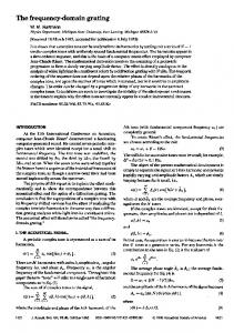
Figure 4. For each rotation angle, the image volume is rotated so that the front face of it always faces the detection plane (viewed along the axis of rotation).

1447

that @ is only a function of ( x p yT). From (16) and (17), we see that the function @ is shift-invariant for a fixed distance Z from the collimator.

projection. Both Steps 1) and 2 ) involve data interpolation. In order to reduce the interpolation errors, Steps 1) and 2) can be combined and data interpolation only needed once.

4.2. Projector with Point Response

4. ROTATION PROJECTOR An iterative EM algorithm [5] is used to reconstruct the images. In each iteration of the algorithm, a projection and a backprojection operation is required. We introduce a rotation projector in this section.

4.1. Rotation Projector The projector used in our implementation is neither raydriven nor voxel-driven. For each rotation angle, we rotate the image matrix volume, so that the front face of the volume always faces the detection plane as shown in Figure 4. We redefine the fixed image relative to the new voxelized matrix. For each angle, the rotation is performed on the image volume at the original position, not at the previous angle, so that the rotation error accumulation is avoided. The projection procedure is illustrated in Figure 5. Let the image volume be x ( i , j , k; m), where m is the angle index, and the detection plane bepG, k; m ) . For the parallel geometry, the projection operation is achieved by layer-by-layer updating:

(18)

p(j,k;m) = x x ( i , j , k m ) . I

For cone beam geometry, x(i,j , k; m ) in (1 8) is replaced by x(i,j’, k’; m),wherej’ and k‘ are calculated along the cone beam ray. Usually j’ and k’ are not integers, and interpolation of the image is required. Similarly, for fan beam geometry, x(i, j , k; m ) in (18) is replaced by x(i, j’, k; m),where j’ is calculated along the fan beam ray. When j’ is not an integer, interpolation is required. Another way to implement a fan beam or a cone beam projector consists of the following three steps: 1) rotate the image volume, 2) warp (scale) the volume so that the projection rays are parallel to each other, and 3 ) use (1 8) to complete the

The rotation projector described in Section 4.1 is convenient to be incorporated with geometric response functions. As proven in Section 3, the geometric response functions are shift-invariant for a fixed depth i. This enables us to implement the model of the geometric response in the frequency domain as a product. This speeds up the geometric point response correction algorithm. The Fourier transform, Q1,of the geometric point response @ is calculated and stored for each depth i. We refer to Ol as the transfer function. We may also include the crystal intrinsic response, which is a Gaussian function, into the transfer function O,. The projector is performed layer by layer. At each layer, we first compute the two-dimensional Fourier transform of layer i in the image volume: X ( i , J, K; m ) = F2[ x(i, j , k; m);j , k ] , where the indices j and k after the semicolon indicate the twodimensional Fourier transform over the indices j and k. Indices J and K are the frequency domain counterparts of indices j and k. Then we multiply X ( i , J, K ; m ) with mi, and compute its twoy (i, j , k ) = dimensional inverse Fourier transform:

yil { X (i, J , K ; m )O lJ;, K } . Finally, y ( i , j , k ) is projected onto p(j, k; m ) as described in Section 4.1. 4.3. Projector with Attenuation A three-dimensional attenuation map p(i, j , k; 1) is required for attenuation correction, where p(i,j, k; 1) is a threedimensional image of the attenuation distribution which can be obtained by transmission tomography. At each angle m, we rotate p(i,j, k; 1) to obtain p(i,j, k; m ) . Let,,i be the index of the layer closest to the detector, and i, be the index of the layer furthest from the detector. For the parallel geometry, the map p(i, j , k; m ) is then summed to give:

I

imax

sum(i,j,k;m) = x p ( l , j , k ; m )

J

axis of rotation

e1 h -

The i,,,th

layer

The ith layer

The i,,,th layer

j Figure 5. Parallel projection is realized by summing up all the layers in the image volume. The index for the layer closest to (or furthest from) the detection plane is imax (or imin).

(19)

I=r

In other words, sum(i,j,k; m ) is formed as a partial line integral of p(i, j , k; m ) . For cone and fan beam geometries, the indices need to be adjusted accordingly. For the parallel geometry, the projector is realized by introducing an attenuation factor e-sum(iJj 2 k ; m, . Thus, (18) becomes P ( j , k ; m ) = c x ( i , j , k ; m )e

-sum (i,j, k ; m )

.

(20)

I

Minor modifications are required for cone and fan beam geometries. On the right hand side of (20), j and k are replaced by J‘ and k‘ for the cone beam geometry, and j is replaced by j’

1448

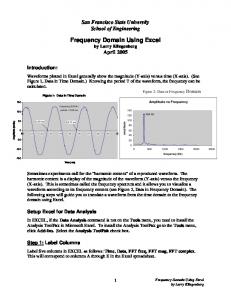
Figure 6. Bit-map representations of the Hoffman three-dimensional brain phantom: T a transverse view, S: a sagittal view, and C: a coronal view. for the fan beam geometry. The actual implementation of the projector combines the model of the geometric response and photon attenuation into one operation.

4.3. Backprojector In an EM algorithm, the projector and the backprojector should have the same model. In other words, if the projection matrix is F, then the backprojection matrix should be FT.In our implementation, the projector and the backprojector use different models in order to save computation time. For example, one uses a ray-driven projector and a voxel-driven backprojector in an EM algorithm. Or, one uses a projector which models the point response function and attenuation, while uses a backprojector which does not models the point response function or attenuation in an EM algorithm. Even different models for the projector and backprojector are used, the modified algorithm should converge to the same result as that of the EM algorithm. In order to see that this is true, let us look at the EM algorithm [ 5 ] :

where XI is the ith voxel in the image volume, Pj is the jth projection bin, and Fljis the contribution of the ith voxel Xi to the jth projection bin Pi. In (21) the summation over k is the projection operation and the summations over j and 1 are the backprojection operations. The summation over 1 is a backprojector which back-projects a constant one. If one uses different models for the projector and the backprojector, algorithm (21) becomes:

I

Table 1. Collimators used in the phantom studies. The hole length is for the central hole of the converging collimators, the hole diameter is the measurement at the center of the tapered hole, and the focal length is measured from the front face of the collimator. The tabulated resolution is the total system resolution (intrinsic plus collimator). Collimator

Resolution (at 10 cm)

Sensitivity

Hole Diameter

Hole. Length

Focal Length

Parallel (PRISM 3000)

7.8 mm

245 cts/min/pCi

1.4 mm

2.7 cm

Fan Beam (PRISM 3000)

7.8 mm

300 cts/min/pCi

1.4 mm

2.7 cm

50 cm

Cone Beam (SX-300)

6.7 mm

252 cts/min/pCi

1.55 mm

3.3 cm

60 cm

00

1449

Figure 7. Parallel beam EM reconstructions. T = transverse view, S = sagittal view, C = coronal view, 1 = collimator geometry, 2 = collimator geometry plus attenuation corrections, 3 = collimator geometry plus point response corrections, and 4 = collimator geometry plus attenuation and point response corrections.

Table 2. Reconstruction Times for Parallel Beam Geometry (120 Views)

1 ~

8021 seconds

Collimator Geometry Collimator Geometry plus Attenuation Corrections

15636 seconds

Collimator Geometry plus Point Response Corrections

15331 seconds

~

Collimator Geometry plus Attenuation and Point Response Corrections

25525 seconds

I I

1450

Figure 8. Fan beam EM reconstructions. T = transverse view, S = sagittal view, C = coronal view, 1 = collimator geometry, 2 = collimator geometry plus attenuation corrections, 3 = collimator geometry plus point response corrections, and 4 = collimator geometry plus attenuation and point response corrections.

Table 3. Reconstruction Times for Fan Beam Geometry (120 Views)

I

9665 seconds

Collimator Geometry Collimator Geometry plus Attenuation Corrections Collimator Geometry plus Point Response Corrections Collimator Geometry plus Attenuation and Point Response Corrections

I

I

17959 seconds 16255 seconds

25453 seconds

1451

Figure 9. Cone beam EM reconstructions. T = transverse view, S = sagittal view, C = coronal view, 1 = collimator geometry, 2 = collimator geometry plus attenuation corrections, 3 = collimator geometry plus point response corrections, and 4 = collimator geometry plus attenuation and point response corrections.

I I 1

Table 4. Reconstruction Times for Cone Beam Geometry (128 Views) Collimator Geometry

19783 seconds

Collimator Geometry plus Attenuation Corrections

33743 seconds

I

Collimator Geometry plus Point Response Corrections

27 174 seconds

I

Collimator Geometry plus Attenuation and Point Response Corrections

I

42897 seconds

I

1452

where G and F may be different models. The convergence of the algorithm implies

collimators listed in Table 1. For the cone beam study on the SX-300, 128 projections were acquired at 60 seconds per projection. For studies performed on the PRISM, 120 projections were acquired at 15 seconds per projection. The parallel data has total counts of 1.85832x107, the fan beam data has total counts of 2.45228x107, and the cone beam data has total counts of 7 . 5 9 2 3 0 ~ 1 0for ~ the central slice in these three geometries.

P . = CFkjX;Id. J

5.2. Image Reconstruction and Results

k

Substituting (23) into (22), we have X y W = xy'd, which means (23) is an equilibrium point of algorithm (22), i.e., algorithm converges to (23). Of course, the reasoning here is heuristic. Since (22) is no longer the EM algorithm (21), the image result from (22) may be different from the image result from (21) after a finite number of iterations. In (22), G is a less accurate model than F which models the point response function and attenuation, while G only models the imaging geometry such as parallel, cone beam, and fan beam. The motivation is to speed up the algorithm. As we will see in the next section that we have equivalent results from (21) and (22), while (22) is much faster than (21).

5. METHODS AND RESULTS 5.1. Phantom and Data Acquisition A physical three-dimensional Hoffman brain phantom was used in our experiments. The phantom was manufactured by Data Spectrum Inc., Hillsborough, North Carolina. The diameter of the phantom is 18 cm, and the length is 15 cm. The phantom was filled with 20 mCi of 99m-Technetium. Bit-map representations of the three-dimensional phantom are shown in Figure 6. Data was acquired by the Picker SX-300 and PRISM SPECT systems. These studies were performed using the

~~

The iterative EM reconstruction algorithm with rotation projector/backprojectorwas coded and results were obtained on an IBM 3090-600s supercomputer. The projections were reconstructed in a 64~64x64matrix. Each reconstruction was obtained after 100 iterations of the EM algorithm. The point response functions were pre-calculated for each layer in the frequency domain. The attenuation coefficient was assumed to be 0.15 cm-' within the phantom. For each parallel, fan beam, and cone beam geometry, we reconstructed four sets of images in which the projector incorporates the collimator geometry, the collimator geometry plus attenuation, the collimator geometry plus the point response, and the collimator geometry plus the point response and attenuation. These reconstructions are shown in Figures 7, 8, and 9 for the parallel, fan beam, and cone beam geometry, respectively. The total reconstruction times are listed in Tables 2, 3, and 4, for parallel, fan beam, and cone beam geometries, respectively. In order to verify the equivalence of algorithm (21) and algorithm (22), we reconstructed another set of images for the fan beam geometry, where both the projector and the backprojector used the same model. We observed that the final images (not shown) are indistinguishable from those images reconstructed with a backprojector which includes the collimator geometry, but does not incorporate with point response nor attenuation. However, the reconstruction times are longer than those listed in Table 3. The fan beam reconstruction times with the same model for the projector and backprojector

~

Table 5. Reconstruction Times for Fan Beam Geometry (120 Views) [The projector and the backprojector have the same model.]

1

Collimator Geometry

1

Collimator Geometry plus Attenuation Corrections

25 111 seconds

1

I

Collimator Geometry plus Point Response Corrections

I

23469 seconds

Collimator Geometry plus Attenuation and Point Response Corrections

I

9665 seconds

38760 seconds

1453

(120 views) are listed in Table S. If we use our previous “inverse cone” ray-driven algorithm [ 101 to reconstruct a three-dimensional fan beam 6 4 ~ 6 4 x 6 4image, the reconstruction time is 1420800 seconds for 120 views, 100 iterations with geometric response and attenuation corrections. This indicates that our frequency domain implementation is about SO times faster than our previous “inverse cone” ray-driven algorithm [ 101.

6. CONCLUSIONS In this paper, a three-dimensional iterative reconstruction algorithm which incorporates models of the geometric point response in the projector-backprojector is presented for parallel, fan, and cone beam geometries. It is shown that the geometric response function is shift-invariant for parallel, fan beam, and cone beam geometries, if the distance from the collimator face is fixed. This property was verified by point source studies before our phantom experiments. This property enabled us to model the system point response function (geometric and intrinsic) in the frequency domain. Compared with our raydriven models [ lo], the frequency domain implementation of the point response function correction significantly reduces the reconstruction time by approximately SO times. Reconstructed images are compared with and without modeling the geometric response and attenuation. Improvements in image quality is shown when the geometric point response and attenuation is appropriately compensated. The modeling of the system response is shown to increase the image resolution, and the attenuation compensation reduces the density nonuniformity artifacts. Our results indicate that the models are good approximations for the physics of the imaging system. In our implementation, the EM algorithm has been modified in such a way that the projector models the imaging geometry, the system point response, and attenuation, while the backprojector models only the imaging geometry. We also reconstructed images with the EM algorithm in which the backprojector also models the system response and attenuation, and we observed that the final images are indistinguishable between these two algorithms after 100 iterations. Object scatter is another source which degrades the image quality, and can be compensated by including its response in the projection operation [ 111.

ACKNOWLEDGMENTS The research work presented in this manuscript was partially supported by NIH Grant R 0 1 HL 39792, the Whitaker Foundation, and Picker Intemational. The authors thank Paul Christian for supplying the phantom data. A grant of computer time from the Utah Supercomputing Institute, which is funded by the State of Utah and the IBM Corporation, is gratefully acknowledged. We also thank Biodynamics Research Unit. Mayo Foundation for use of the Analyze software package.

REFERENCES [l] C. E. Metz, E B. Atkins and R. N. Beck, “The geometric transfer

function component for scintillation camera collimators with straight parallel holes”, Phys. Med. Biol., Vol. 25, pp. 1059-1070, 1980. [2] B. M. W. Tsui and G. T. Gullberg,“The geometric transfer function for cone and fan beam collimators,”Phys. Med. Biol., Vol. 35, pp. 81-93, 1990. [3] T. E Budinger, G. T. Gullberg, and R. H. Huesman, “Emission computed tomography,” in Image Reconstruction From Projections, Springer-Verlag,New York, 1979,pp. 147-246. [4] L. A. Shepp, and Y. Vardi, “Maximum likelihood reconstruction for emission tomography,”IEEE Trans. Med. Imag., vol. 1,pp. 113122,1982. [5] K. Lang and R. Carson, “EM reconstruction algorithms for emission and transmission tomography,” J . Comput. Assist. Tomogr., vol. 8, pp. 306-316, 1984. [6] B. M. W. Tsui, H. B. Hu, D. R. Gilland, and G. T. Gullberg, “Implementation of simultaneous attenuation and detector response correction in SPECT,” IEEE Trans. on Nucl. Sci., vol. 35, pp. 778-783, 1988. [7] A. R. Formiconi, A. Pupi, and A. Passeri, “Compensation of spatial system response in SPECT with conjugate gradient reconstruction technique,”Phys. Med. Biol., vol. 34, pp. 69-84, 1989. [8] C. E. Floyd, R. J. Jaszczak, S. H. Manglos, and R. E. Coleman, “Compensation for collimator divergence in SPECT using inverse Monte Carlo reconstruction,” IEEE Trans. Nucl. Sci., vol. 35, pp. 784-787, 1988. [9] B. C. Penney, M. A. King, and K. Knesaurek, “A projector, backprojector pair which accounts for the two-dimensional depth and distance dependent blurring in SPECT,”IEEE Trans. Nucl. Sci., vol. 37, pp. 681-686, 1990. [ 101 G. L. Zeng, G. T. Gullberg, B. M. W. Tsui, and J. A. Terry, “Threedimensional iterative reconstruction algorithms with attenuation and geometric point response correction,” IEEE Trans. Nucl. Sei., vol. 38, pp. 693-702, 1991. [ 111 Z. Liang, R. J. Jaszczak, T. G. Turkington, D. R. Gilland and R. E. Coleman, “Simultaneous compensation for attenuation, scatter, and detector response of SPECT reconstruction in three dimensions,”Phys. Med. Biol., 1992, pp. 587-603.