Abstract. Filtering is critical for representing detail, such as color textures or normal maps, across a variety of scales. While MIP-mapping tex- ture maps is ...
Frequency Domain Normal Map Filtering Charles Han
Bo Sun
Ravi Ramamoorthi Columbia
Eitan Grinspun
University∗
Abstract Filtering is critical for representing detail, such as color textures or normal maps, across a variety of scales. While MIP-mapping texture maps is commonplace, accurate normal map filtering remains a challenging problem because of nonlinearities in shading—we cannot simply average nearby surface normals. In this paper, we show analytically that normal map filtering can be formalized as a spherical convolution of the normal distribution function (NDF) and the BRDF, for a large class of common BRDFs such as Lambertian, microfacet and factored measurements. This theoretical result explains many previous filtering techniques as special cases, and leads to a generalization to a broader class of measured and analytic BRDFs. Our practical algorithms leverage a significant body of work that has studied lighting-BRDF convolution. We show how spherical harmonics can be used to filter the NDF for Lambertian and low-frequency specular BRDFs, while spherical von MisesFisher distributions can be used for high-frequency materials.
zoomed in
(a) V-groove
(b)
(d) NDF
NDF
(c) V-groove (e) standard
BRDF
effective BRDF (f) convolution
zoomed out
Figure 1: Consider a simple V-groove. Initially in closeup (a), each face is a single pixel. As we zoom out, and average into a single pixel (c), standard MIP-mapping averages the normal to an effectively flat surface (e). However, our method uses the full normal distribution function or NDF (d), that preserves the original normals. This NDF can be linearly convolved with the BRDF (f) to obtain an effective BRDF, accurate for shading.
1 Introduction Representing surface detail at a variety of scales requires good filtering algorithms. For texture mapping, there has been considerable effort at developing and analyzing filtering methods [Heckbert 1989]. A common, linear approach to reduce aliasing is MIPmapping [Williams 1983]. Normal mapping (also known as bump mapping [Blinn 1978] or normal perturbation), a simple and widely used analogue to color texture mapping, specifies the surface normal at each texel. Unfortunately, normal map filtering is very difficult because shading is not linear in the normal. For example, consider the simple V-groove surface geometry in Fig. 1a. In a closeup, this spans two pixels, each of which has distinct normals (b). As we zoom out (c), the average normal of the two sides (e) corresponds simply to a flat surface, where the shading is likely very different. By contrast, our method preserves the full normal distribution (d) in the spirit of [Fournier 1992], and shows how to convolve it with the BRDF (f) to get an accurate result. A more complex example is Fig. 2, which compares our method with “ground truth”1 , standard MIP-mapping of normals, and the recent normal map filtering technique of [Toksvig 2005]. At close range (top row), minimal filtering is required and all methods perform identically. However, as we zoom out (middle and especially bottom rows), we quickly obtain radically different results. It has long been known qualitatively that antialiasing involves convolution of the input signal (here, the distribution of surface ∗ {charhan,bosun,ravir,eitan}@cs.columbia.edu URL: http://www.cs.columbia.edu/cg/normalmap 1 “Ground truth” images are obtained using jittered supersampling (on the order of hundreds of samples per pixel) and unfiltered normal maps.
Figure 2: Top: Closeup of the base normal map; all other methods are identical at this scale and are not shown. Schematic (a) and diffusely shaded (b) views are provided to aid in comparison/visualization. Middle: When we zoom out, differences emerge between our (6-lobe) spherical vMF method, the Toksvig approach (rightmost), and normalized MIPmapping. (Unnormalized MIP-mapping of normals produces an essentially black image.) Bottom: Zooming out even further, our method is clearly more accurate than Toksvig’s model, and compares favorably with ground truth. (The reader may zoom into the PDF to compare images.)
normals) and an appropriate low-pass filter. Our most important contribution is theoretical, formalizing these ideas and developing a comprehensive framework for normal map filtering. In Sec. 4, we derive an analytic formula, showing that filtering can be written as a spherical convolution of the BRDF of the material with a function we define as the normal distribution function (NDF)2 of the texel. This mathematical form holds for a large class of common BRDFs including Lambertian, Blinn-Phong, microfacet models like Torrance-Sparrow, and many measured BRDFs. However, the convolution does not apply exactly to BRDF models that 2 We define the NDF as a weighted mapping of surface normals onto the unit sphere; more formally, it is the extended Gaussian Image [Horn 1984] of the geometry within a texel.
Acronym NDF SH SRBF EM vMF movMF
Definition normal distribution function spherical harmonics spherical radial basis function expectation maximization von Mises-Fisher distribution mixture of vMF lobes
Symbol γ (n) Ylm γ (n · µ )
γ (n · µ ; θ ), θ = {κ , µ } γ (n; Θ), Θ = {α j , θ j }Jj=1
Table 1: Important abbreviations and acronyms used in the paper.
depend on the “reflected direction” between the light source and viewer, e.g., the standard Phong model. Our analytic result immediately connects geometrical normal map filtering with the older lighting-BRDF convolution result for appearance [Basri and Jacobs 2001; Ramamoorthi and Hanrahan 2001]. This result also unifies many previous normal map filtering approaches, which can now be viewed as special cases. Moreover, we can immediately apply a host of mathematical representations originally developed for lighting-BRDF convolution. In particular, we develop two novel algorithms. Our first method (Sec. 5) is a general framework that uses spherical harmonics (SH). Although general, this method is most suitable for low-frequency BRDFs, where it suffices to use a small number of SH coefficients. Our second method, intended for high-frequency materials, uses an approximate function fitting technique known as spherical expectation maximization (EM) [Banerjee et al. 2005]. This method approximates or fits the NDF with von Mises-Fisher (vMF) distributions (Sec. 7). vMFs are spherical Gaussian-like functions, symmetric about a central direction (average normal). To our knowledge, the use of vMFs and spherical EM is new in graphics, and may have broader relevance. Finally, our framework enables realistic BRDFs, including measured materials (Fig. 4), as well as dynamically changing reflectance, lighting and view (Fig. 8). We are also able to incorporate low-frequency environment maps (Fig. 9). Although this paper presents an in-depth theoretical discussion, the final algorithms are relatively simple. Readers more interested in implementation may wish to pay special attention to Sec. 5.1, that describes the spherical harmonic method, and the full pseudocode provided in Algorithms 1 and 2 for the vMF method of Sec. 7. Additionally, videos and example GLSL shader code for all of our results are available for download from our website.
2 Previous Work Normal Map Filtering: Many previous methods approximate the normal distribution function using a single symmetric or asymmetric lobe. [Schilling 1997] described the lobe using covariance matrices, while [Olano and North 1997] mapped normal distributions consisting of a single 3D Gaussian. A simple GPU method is described in [Toksvig 2005]. In our framework, these methods can retrospectively be considered similar to using a single vMF lobe. As seen in Figs. 2 and 7, one lobe is insufficient for complex NDFs. An early inspiration is [Fournier 1992], which uses up to seven Phong lobes per texel (and up to 56 at the coarsest scales). This can be seen as a special case of our framework, with some similarities to our spherical vMF algorithm. Note that [Fournier 1992] uses nonlinear least-squares optimization to fit lobes. In our experience, this is unstable and slow, especially considering the number of peaks and texels in a normal map. vMFs are very similar to Gaussian or Phong lobes, but have many technical advantages, in allowing for fast and robust fitting using existing algorithms for spherical EM. The most recent and closest previous work is [Tan et al. 2005], which uses EM to fit Gaussian lobes to a planar projection of the hemispherical NDF at each texel. We introduce a new theoretical result in terms of the analysis of normal map filtering as
convolution—it is easy to understand [Tan et al. 2005] as an important special case in this framework. Our formulation also allows spherical harmonic methods for low-frequency materials and Lambertian objects, which do not even require non-linear fitting of lobes. For high-frequency materials we use vMFs and spherical EM, which operate in the natural spherical domain of surface normals; by contrast, planar Gaussian fits, as in [Tan et al. 2005], have been shown to considerably reduce accuracy both in our work (Fig. 7) and in other contexts [Strehl et al. 2000]. Note that [Tan et al. 2005] treat the BRDF itself as a pre-baked distribution of normals at fine-scale texels. We support and discuss this multi-scale tradeoff between BRDF and geometry (Sec. 6.2). However, our spherical representation enables us to derive a formal convolution result of the NDF with the BRDF, and allows us to separate or factor the two. The same NDF can be used with different, possibly non-Gaussian BRDFs, easily. We can also change the BRDF at runtime, and support dynamic, low-frequency complex lighting. Hierarchy of Representations: A hierarchy of scales, with geometry transitioning to bump or normal maps, transitioning to BRDFs, was first proposed by Kajiya [1985]. This idea is explored in detail by [Becker and Max 1993], but they do not focus on normal map filtering as in our work. Similarly, appearance-preserving simplification methods replace fine-scale geometry with normal and texture maps [Cohen et al. 1998]. It is likely that our approach could enable continuous level of detail and antialiasing in these methods. Separately, our formulation allows one to understand the tradeoff between a normal distribution and the BRDF, since the final image is given by a convolution of the NDF and BRDF. Convolution and Precomputed Radiance Transfer (PRT): Many of our mathematical representations and ideas derive from previous spherical convolution techniques [Basri and Jacobs 2001; Ramamoorthi and Hanrahan 2001]. We also build on PRT methods that have used spherical harmonics [Sloan et al. 2002]. Our spherical vMF method extends zonal harmonics [Sloan et al. 2005] and spherical radial basis functions [Tsai and Shih 2006]. We also considered wavelet methods (introduced for reflectance in [Lalonde and Fournier 1997]), but found the number of terms for an artifact-free solution too large for practical use, even with smoother wavelets.3 A real-time method for wavelet-based BRDF representation and filtering on the GPU is given in [Claustres et al. 2007], which does not account for normal map filtering. We emphasize, however, that ours is not a PRT algorithm; it requires minimal precomputation and works with conventional realtime rendering techniques. Furthermore, our method rests on an explicit analytic convolution formula and uses the representations above solely for normal map filtering, not for PRT.
3
Preliminaries
In this section, we introduce relevant notation for the reflectance equation, and BRDF and normal map representations. Note that in this paper, we focus only on normal map filtering and do not consider displacement maps, occlusion, masking, geometry simplification or cast shadows—filtering these additional effects is an important direction of future work (and discussed in Sec. 9). The reflected light B at a spatial point x in direction ω o is B(x, ω o ) =
Z
S2
L(x, ω i )ρ (ω ′i , ω ′o ) d ω i ,
(1)
where L is the lighting at x from incident direction ω i , and ρ is the BRDF (actually, the transfer function including the cosine of the incident angle). Most generally we must integrate over the sphere S2 3 PRT
methods can use a coarse wavelet approximation of the lighting, since it is not visualized directly, but we directly visualize NDF and BRDF.
of incident directions, but in this paper L will usually be assumed to be from a small number of point lights, making equation 1 a summation over discrete directions ω i . We will relax this restriction, and discuss extensions to environment maps, in Sec. 8. Equation 1 is the standard reflectance equation. However, we have made explicit that ω ′i and ω ′o are the local directions in the surface coordinate frame (in which the BRDF is defined). To find them, we must project or rotate the global incident and outgoing directions ω i and ω o to the local tangent frame. This local frame is defined by the surface normal n and a tangent direction. In this paper, we limit ourselves to isotropic BRDFs, so the tangent direction is not important, and we can use any rigid rotation Rn mapping the normal to the z-axis [Ramamoorthi and Hanrahan 2001],
ω ′i
= Rn (ω i )
ω ′o
= Rn (ω o ).
3.1 BRDF Representation and Parameterization
Effective BRDF: We define a new function, the effective BRDF or transfer function that depends on the surface normal (that we denote as n(x) or simply n for clarity) as,
ρ eff (ω i , ω o ; n) = ρ (Rn (ω i ), Rn (ω o )) ,
B(x, ω o ) =
S2
eff
L(x, ω i )ρ (ω i , ω o ; n(x)) d ω i .
BRDF Parameterizations:
(2)
Many BRDFs can be written as
ρ eff (ω i , ω o ; n) = f (n · ω (ω i , ω o )),
=
1 N
=
Z
∑
Z
2 q∈x S
S2
L(x, ω i )ρ eff (ω i , ω o ; n(q)) d ω i 1 N
L(x, ω i )
!
∑ ρ eff (ω i , ω o ; n(q)) d ω i .
q∈x
This formulation allows us to define a new effective BRDF, � � 1 ρ eff (ω i , ω o ; x) = ∑ ρ Rn(q) (ω i ), Rn(q) (ω o ) . N q∈x
(4)
Note that the effective BRDF now depends implicitly on all the normals n(q) at x, rather than on a single normal. This paper is about efficiently computing and representing ρ eff . The next section shows how to explicitly represent ρ eff as a convolution of the original BRDF and a new function we call the NDF.
Theory of Normal Mapping as Convolution
In this section, we introduce our theoretical framework for normal map filtering as convolution. The next sections describe mathematical representations that can be used for practical implementation. 4.1 Normal Distribution Function (NDF)
(3)
where the 1D function f is radially symmetric about the shading normal n, and depends on the chosen parameterization ω (ω i , ω o ) (henceforth ω ). In this paper, we focus most of our effort on these types of BRDFs, which encompass Lambertian, Blinn-Phong or microfacet half angle (like Torrance-Sparrow), and many factored and measured BRDFs. A very common example is Lambertian reflectance, where the transfer function is simply the cosine of the incident angle, so that ω = ω i , and f (u) = max(u, 0). The Blinn-Phong specular model with exponent s uses a transfer function of the form f (u) = us , with i +ω o the half-angle parameterization, ω = ω h = kω ω +ω k . Measured i
B(x, ω o )
4
allowing us to write equation 1 using the global directions, Z
Normal Map Filtering: In screen space, the exitant radiance or pixel color B(x, ω o ) at a surface location x should represent the average radiance at the N corresponding finer-level texels q:
o
BRDF functions f (ω h · n) can also be used.4
3.2 Normal Map Representation and Filtering Normal Map Input Representation: There are many equivalent normal map representations, including bump maps [Blinn 1978] and normal offsets. For simplicity, we use normal maps, parameterized on a plane, that directly specify the normal in tangent space. In the actual implementation, we perform all computations in the local tangent frame of the geometric surface; lighting and view are projected into this local frame, allowing the planar normal map to be used directly without explicit rotation. For simplicity in the proceeding discussion, the reader can therefore assume a planar underlying surface while understanding that the extension to curved 3D geometry is straightforward. For memory and practicality reasons, normal maps do not typically use resolutions much higher than 512 × 512 or 1024 × 1024. To obtain effectively higher or finer resolutions, we therefore often tile the base normal map over the surface. 4 A number of recent papers have proposed factored BRDFs for measured reflectance. [Lawrence et al. 2006] uses a factorization f (θh )g(θd ), in terms of half and difference angles. The f (θh ) term clearly fits into the framework of equation 3, but the BRDF now also includes a product with g(θd ). However, θd does not depend on n (and g does not need to be filtered). Thus, our framework also applies to general BRDFs of the form f (ω · n)g(ω i , ω o ), where the g factor does not depend directly on n.
Our first step is to convert equation 4 into continuous form, defining
ρ eff (ω i , ω o ; γ (·)) =
Z
S2
ρ (Rn (ω i ), Rn (ω o )) γ (n) dn,
(5)
where γ (n) is a new function that we introduce and define as the normal distribution function (NDF), and the integral is over the sphere S2 of surface orientations. Note that a unique NDF γ (n) exists at each surface location x; for a discrete normal map, γ (n) would simply be a sum of (spherical) delta distributions at n(q), the fine-scale normals at x. Formally, γ (n) = N1 ∑q∈x δ (n − n(q)), as seen in Fig. 1d. For some procedurally generated normal maps, γ (n) may be available analytically. 4.2 Frequency Domain Analysis in 2D
Although we will not directly use the results of this section for rendering, we can gain many insights by starting in the simpler 2D case. This “flatland” analysis is easier because the rotation operator in equation 5 is given simply by Rn (ω ) = ω + n, yielding
ρ eff (ωi , ωo ; γ (·)) =
Z 2π 0
ρ (ωi + n, ωo + n) γ (n) dn.
(6)
Significant new insight is gained by analyzing equation 6 in the frequency domain. Specifically, we expand in Fourier series:
γ (n)
=
∑ γk Fk (n) k
ρ (ωi + n, ωo + n)
=
∑ ∑ ρlm Fl (ωi + n)Fm (ωo + n),
(7)
l m
where Fk (n) are the familiar Fourier basis functions √1 eikn . Not2π √ ing that Fk (ω + n) = 2π Fk (ω )Fk (n), equations 6 and 7 can be simplified to
ρ eff (ωi , ωo ; γ (·))
=
2π
∑ γk ρlm Fl (ωi )Fm (ωo ) ×
k,l,m
Z 2π 0
Fk (n)Fl (n)Fm (n)dn.
(8)
“Ground truth”
The integral above involves a triple integral of Fourier series, and we denote the corresponding tripling coefficients Cklm . These tripling coefficients have recently been studied in [Ng et al. 2004], and for Fourier series they vanish unless k = −(l + m), where Cklm = √1 . Since ρ eff above is already expressed in terms of 2π Fl (ωi )Fm (ωo ), we can write a formula for its Fourier coefficients: √ eff (9) ρlm = 2πγ−(l+m) ρlm . Discussion and Analogy with Convolution: Equation 9 gives a very simple product formula for the frequency coefficients of the effective BRDF. This is much like a convolution, where the final Fourier coefficients are a product of the Fourier coefficients of the functions being convolved (here the NDF and BRDF). However, the convolution analogy is not exact, since equation 8 involves a triple integral and n appears thrice in equation 6. In 3D, the formulae and sparsity for triple integrals in the frequency domain (especially those involving rotations) are much more complicated [Ng et al. 2004]. Fortunately, many BRDFs are primarily single-variable functions f (ω · n) as in equation 3. In these cases, we will obtain a spherical convolution of the NDF and BRDF.
Our method
Standard anisotropic filtering
Figure 3: Spherical harmonic anisotropic filtering for Lambertian reflection. Note the behavior for far regions of the plane. With standard normal filtering, these regions are averaged to a nearly flat surface. By contrast, our method is quite accurate in distant regions.
4.3 Frequency Domain Analysis in 3D
To proceed with analyzing equation 5 in the 3D case, we substitute the form of the BRDF from equation 3. Recall in this case that the BRDF only depends on the angle between ω and the surface normal n, and is given by f (ω · n). The effective BRDF is now also only a function of ω ,
ρ eff (ω ; γ (·)) =
Z
S2
f (ω · n)γ (n) dn.
(10)
Note that the initial BRDF ρ (·) = f (ω · n) is symmetric about n, but the final result ρ eff (ω ) is an arbitrary function on the sphere and is generally not symmetric. We would like to analyze equation 10 in the frequency domain, just as we did with equation 6. In 3D, we must use the spherical harmonic (SH) basis functions Ylm (·), which are the frequency domain analog to Fourier series on the unit sphere. The l index is the frequency with l ≥ 0, and −l ≤ m ≤ l, ∞
γ (n) =
∞
l
∑ ∑ l=0 m=−l
γlmYlm (n)
∑ fl Yl0 (ω · n)
f (ω · n) =
l=0
ρ eff (ω ) =
∑ ∑
∞
l
eff Ylm (ω ). ρlm
l=0 m=−l
The above is a standard function expansion, as in Fourier series. Note that the symmetric function f (ω · n) is expanded only in terms of the zonal harmonics Yl0 (·) (m = 0), which are radially symmetric and thus depend only on the elevation angle. Equation 10 has been extensively studied in recent years, within the context of lighting-BRDF convolution for Lambertian or radially symmetric BRDFs [Basri and Jacobs 2001; Ramamoorthi and Hanrahan 2001]. In those works, the NDF γ (n) is replaced by the incident lighting environment map. Since the theory is mathematically identical, we may directly use their results. Specifically, equation 10 expresses a spherical convolution of the NDF γ (n) with the BRDF filter f . In particular, there is a simple product formula in spherical harmonic coefficients, similar to the way standard convolution can be expressed as a product of Fourier coefficients, r 4π eff fγ . ρlm = 2l + 1 l lm Explicitly making the NDF and effective BRDF functions of a texel q, we have
eff ρlm (q) = ρˆ l γlm (q)
ρˆ l =
r
4π f , 2l + 1 l
(11)
where the NDF considers all normals covered by q. While q usually corresponds to a given level and offset in a MIP-map, it can also consider more general “footprints”—we show an example with anisotropic filtering in Fig. 3. Generality and Supported BRDFs: The form above is accurate for all BRDFs described by equation 3, including Lambertian, Blinn-Phong and measured microfacet distributions. Moreover, our results also apply when the BRDF has an additional Fresnel or g(θd ) multiplicative factor, since θd (and hence g) does not depend on n and does not need to be filtered. Note that for some specular BRDFs, we also need to multiply by the cosine of the incident angle for a full transfer function. For the spherical vMF method in Sec. 7, we address this by simply multiplying for each lobe by the cosine of the angle between light and lobe center (or effective normal). For the spherical harmonic method in Sec. 5, we simply use the MIP-mapped normals for the cosine term, since it is a relatively low-frequency effect.
5
Spherical Harmonics
To recap, we have as input a normal map which provides a single normal n(q0 ) for each finest-level texel q0 . We also have a BRDF ρ (·) = f (ω · n), with spherical harmonic coefficients ρˆ l . In this section, we develop a spherical harmonics-based algorithm from the final formula in equation 11. Later, Sec. 7 will discuss an alternative algorithm better suited for higher-frequency effective BRDFs. While the theory in the previous section is somewhat involved, the practical algorithm in this section is relatively straightforward, involving two basic steps: (1) computing the NDF spherical harmonic coefficients γlm (q) for each (coarse-level) texel q of the normal map, and (2) rendering the final color by directly implementing equation 11 in a GPU pixel shader. 5.1 Algorithm
Computing NDF Coefficients: We compute a MIP-map of NDF coefficients5 , starting with the finest level normal map, and moving 5 As explained in Sec. 3.2, we are operating in the local tangent frame of the geometric surface, with lighting and view projected into this frame. Thus, we do not need to explicitly consider rotations into the global frame. Note that the overall geometric surface is assumed to be locally planar (a
to coarser levels. At the finest level (denoted by subscript 0), γ (q0 ) is a delta distribution at n(q0 ), i.e., γ (q0 ) = δ (n − n(q0 )) with corresponding spherical harmonic coefficients6
γlm (q0 ) = Ylm (n(q0 )). An important insight is that, unlike the original normals, these spherical harmonic NDF coefficients γlm (q0 ) can now correctly be linearly filtered or averaged for coarser levels γlm (q). Hence, we can simply MIP-map the spherical harmonic coefficients γlm (q0 ) in the standard way, and no non-linear fitting is required. Rendering: Rendering requires knowing the NDF coefficients γlm (q), the BRDF coefficients ρˆ l , and then applying equation 11. We have already computed a MIP-map of NDF coefficients. At the time of rendering, we also know the BRDF. For many analytic models, formulae for ρˆ l are known [Ramamoorthi and Hanrahan 2 2001]. For example, for Blinn-Phong, ρˆ l ∼ e−l /2s where s is the Phong exponent. For measured reflectance, ρˆ l is obtained directly by a spherical harmonic transform of f (ω · n). Now, we can compute the spherical harmonic coefficients of the effective BRDF, per equation 11. Finally, to evaluate it, we must expand in terms of spherical harmonics,
ρ eff (ω , q) =
l∗
l
∑ ∑
ρˆ l γlm (q)Ylm (ω ),
(12)
l=0 m=−l
where ω (ω i , ω o ) depends on the BRDF as usual (such as incident direction ω = ω i for Lambertian or halfway-vector ω = ω h for specular), and l ∗ is the maximum √ l used in the shader (accurate results generally require l ∗ ∼ 4s where s is the Blinn-Phong exponent). For shading, assume a single point light source for now. At each surface location, we know the incident and outgoing directions, so it is easy to find the half-vector ω h or other parameterization ω , and then use the BRDF formula above for rendering.7 We implement equation 12 in a pixel shader using GLSL (see our website for example code). The spherical harmonics Ylm are stored in floating point textures, as are the MIP-mapped NDF coefficients γlm (q). Real-time frame rates are achieved comfortably for up to 64 spherical harmonic terms (l ∗ ≤ 7, corresponding to a Blinn-Phong exponent s ≤ 12 or a Torrance-Sparrow surface roughness σ ≥ 0.2). 5.2 Results
Lambertian Reflection: In the Lambertian case, using only nine spherical harmonic coefficients (l ≤ 2) suffices [Ramamoorthi and Hanrahan 2001]. An example is shown in Fig. 3. This figure also shows the generality of our method in terms of the footprint for texel q, by using GPU-based anisotropic filtering, instead of MIPmapping. Note that we preserve accuracy in far away regions of the plane, while naïve averaging of the normal produces a nearly flat surface that is much darker than the actual (as illustrated in Fig. 1e). Low-Frequency Specularities and Measured Reflectance: Specular materials with BRDF f (ω h · n) also fit within our framework. The BRDF can also be changed at run-time, since the NDF is independent of it. We have factored all of the materials in the database of [Matusik et al. 2003], using the f (θh )g(θd ) factorization in [Lawrence et al. 2006]. Figure 4 shows two examples of different materials, which we can switch between at runtime. Figure 5 shows closeup views from an animation sequence of cloth draping over a sphere, using the blue fabric material from the single “geometric normal”) over the region being filtered. 6 We use the real form of the spherical harmonics, rather than the com∗ (n(q )). plex form, to simplify implementation. Otherwise, γlm (q0 ) = Ylm 0 7 Our spherical harmonic algorithm does not explicitly address color textures; a simple approximation would be to MIP-map them separately, and then modulate the scalar result in equation 12. A more correct approach to filtering material properties is discussed for our vMF method in Sec. 7.3.
“Leather”
“Violet Rubber”
Figure 4: Our spherical harmonic algorithm for normal mapping, with two of the materials in the Matusik database—we can support general measured BRDFs and change reflectance or material in real time. Notice also the correct filtering of the zoomed out view, shown at the bottom right.
Matusik database. Note the accuracy of our method (compare (b) with the supersampled “ground truth” in (c)). Also note the smooth transition between close (unfiltered) and distant (fully filtered) regions in (a) and (b), as well as the filtered zoomed out view in (d). Discussion and Limitations: Our spherical harmonic method is a practical approach for low-frequency materials. Unlike previous techniques, all operations are linear—no nonlinear fitting is required, and we can handle arbitrary lobe shapes and functions f (ω h · n). Moreover, the BRDF is decoupled from the NDF, enabling simultaneous changes of BRDF, lighting and viewpoint. As with all low-frequency approaches, our spherical harmonic method requires many terms for high-frequency specularities (a Blinn-Phong exponent of s = 50 needs about 200 coefficients). The following sections provide more practical solutions in these cases.
6
Spherically Symmetric Distributions
Spherical harmonics are a suitable basis for representing lowfrequency functions, but are impractical for higher-frequency functions due to the large number of coefficients required. For higherfrequency NDFs, then, we will instead use radially symmetric basis functions, which are one-dimensional and therefore much more compactly represented. By performing an offline optimization, we approximate the NDF at each texel as the sum of a small number of such lobes. Our approach is inspired by the symmetric Phong lobes used in [Fournier 1992], and effectively formalizes that method within our convolution framework. 6.1 Basic Theoretical Framework for using SRBFs
Consider a single basis function γ (n · µ ) for the NDF, symmetric about some central direction µ . For now, γ is a general spherical radial basis function (SRBF). Equation 10 now becomes
ρ eff (ω · µ ; γ (·)) =
Z
S2
f (ω · n)γ (n · µ ) dn.
It can be shown (for example, see [Tsai and Shih 2006]) that ρ eff is itself radially symmetric about µ (hence the form ρ eff (ω · µ ) above), and its spherical harmonic coefficients are given by
ρleff = ρˆ l γl .
(13)
Compared to equation 11, this is a simpler 1D convolution, since all functions are radially symmetric and therefore one-dimensional. To represent general functions, we can use a small number of representative lobes γl, j . Note that the calculation of the lobe directions
(a) Our method, frame 1
(b) Our method, frame 2
( c ) “ G r o u n d t r u t h ”, f r a m e 2
(d) Our method, zoomed out
Figure 5: Stills from a sequence of cloth draping over a sphere, with closeups indicating correct normal filtering using our spherical harmonic algorithm (the full movie is shown in the video). Note the smooth transition from the center (almost no filtering) to the corners (fully filtered) in (b)—compare also with ground truth in (c). (d) is a zoomed out view that also filters correctly. We use a blue fabric material from the Matusik database as the BRDF.
is generally a nonlinear process; our particular implementation is given in Sec. 7. For rendering, we need to expand the effective BRDF in spherical harmonics, analogously to equation 12, but now using only the m = 0 terms. Considering the summation of J lobes, we obtain
ρ eff (ω , q) =
J
∞
∑ ∑ ρˆl γl, j (q)Yl0 (ω · µ j ),
(14)
j=1 l=0
where we again make clear that the NDF γl, j is a function of the texel q. This equation can be used directly for shading once we find ω for the light source and view direction. 6.2 Discussion: Unifying Framework and Multiscale
Our theoretical framework in Sec. 6.1 unifies many normal filtering algorithms. Previous lobe- or peak-fitting methods can be seen as special cases. For instance, [Schilling 1997; Toksvig 2005] effectively use a single lobe (J = 1), while [Fournier 1992] uses multiple Phong lobes for γ (n · µ ). These methods have generally adopted simple heuristics in terms of the BRDF. By developing a general convolution framework, we show how to separate the NDF from the BRDF. Since we properly account for general BRDFs ρˆ l , we can even change BRDFs on the fly—in contrast, even [Tan et al. 2005] is limited to predetermined Gaussian Torrance-Sparrow BRDFs. Equation 13 has an interesting multi-scale interpretation, as depicted in Fig. 6. At the finest scale (a), the geometry used is the original highest-resolution normal map. Therefore, the NDF is a delta distribution at each texel, and the effective BRDF ρleff = ρˆ l . At coarser scales, the shading geometry used is effectively a filtered version of the fine-scale normal map, with the NDF becoming smoother from (b)-(d). The effective BRDF is now filtered by the smoothed NDF, essentially representing the complex fine-scale geometry as a blurring of the BRDF. Also note the symmetry between the BRDF and NDF in equation 13. While the common fine-scale interpretation is for a delta function NDF and the original BRDF, we can also view it as a delta function BRDF and an NDF given by ρˆ l . These interpretations are consistent with most microfacet BRDF models, which start by assuming a mirror-like BRDF (delta function) and complex NDF (microfacet distribution), and derive a net glossy BRDF on a smooth macrosurface (delta function NDF). 6.3 Choice of Radial Basis Function
We now briefly discuss some possible approaches for approximating and representing our radial basis functions γ (n · µ ). One possible method is to use zonal harmonics [Sloan et al. 2005]; however, our high-frequency NDFs lead to large orders l, making fitting difficult and storage inefficient. An alternative is to use Gaussian RBFs, with parameters chosen using expectation maximization (EM) [Dempster et al. 1977]. In this case, we simply need to store 3 parameters per SRBF: the amplitude, width and central direction. Whereas [Tan et al. 2005] pursued this approach using Euclidean
Figure 6: Illustration of multiscale filtering of the BRDF (rendered sphere) and NDF (inset). (a) shows a closeup of the sphere, where we see the individual facets and a sharp NDF/effective BRDF. In (b), we have zoomed out to where the geometry now appears smoother, although roughness is still clearly visible. The effective BRDF is now blurred, now incorporating finer-scale geometry. As we zoom further out in (c) and (d), the geometry appears even smoother, while the BRDF is further filtered.
or planar (and therefore distorted) RBFs, we consider NDFs represented on their natural spherical domain, which also enables us to derive a simple convolution formula. Indeed, spherical Gaussian RBFs, such as in [Tsai and Shih 2006] or Phong lobes, as in [Fournier 1992], are most appropriate. However, the nonlinear minimization required for fitting these models is inefficient, given that we need to do so at each texel. Instead, we use a spherical variant [Banerjee et al. 2005] of EM, with the von Mises-Fisher8 (vMF) distribution [Fisher 1953]. Spherical EM and vMFs have previously been used in other areas such as computer vision [Hara et al. 2005] for approximating TorranceSparrow BRDFs; here we introduce them for the first time in computer graphics, to represent NDFs.
7
Spherical vMF Algorithm
We now describe our algorithms for fitting the NDF, and rendering with mixtures of vMF lobes. The fitting is done using a technique 8 For the unit 3D sphere, this function is also known as the Fisher distribution. We use the more general term von Mises-Fisher distribution, that applies to n-dimensional hyperspheres.
known as spherical expectation maximization (EM) [Banerjee et al. 2005]. EM is a common algorithm for fitting in statistics, that finds “maximum likelihood” estimates of parameters [Dempster et al. 1977]. It is an iterative method, with each iteration consisting of two steps known as the E-step and the M-step. We use EM as opposed to other fitting and minimization techniques because of its simplicity, efficiency, robustness, and ability to work with sparse data (the discrete normals in the NDF). We also show how to extend the basic spherical EM algorithm to handle color and different materials, create coherent lobes for hardware interpolation, and implement spherical harmonic convolution for rendering. Note that while the theoretical development of this section is somewhat complicated, the actual implementation is quite simple, and full pseudocode is provided in Algorithms 1 and 2. 7.1 Fitting NDF with Mixtures of vMFs
κ eκ (n·µ ) . 4π sinh(κ )
(15)
A mixture of vMFs (movMF) is defined as an affine combination of vMF lobes θ j , with amplitude α j , where ∑ j α j = 1, J
γ (n; Θ) =
∑ α j γ j (n · µ j ; θ j ).
j=1
Here, θ j = {κ j , µ j } characterizes a single vMF lobe, and Θ stores the parameters {α j , θ j }Jj=1 of all J vMFs in the movMF. We use spherical EM (Algorithm 1) to fit a movMF to the normals covered at each texel in the MIP-map. Line 5 of Algorithm 1 shows the E-step. For all normals ni in a given texel, we compute the expected likelihood hzi j i that ni corresponds to lobe j. Lines 914 execute the M-step, which computes maximum likelihood estimates of the parameters. In practice, we seldom need more than 10 iterations, so the full EM algorithm for a 512 × 512 normal map converges in under 2 minutes. Note that this is an offline computation that needs to be done only once per normal map—unlike most previous work, it is also independent of the BRDF (and lighting). Note the use of auxiliary variable r j in line 11, which represents hx j i/α j , where hx j i is the expected value of a random vector generated according to the scaled vMF distribution γ (x; θ j ). The central normal µ j and the inverse width κ j are related to r j by r
=
A(κ )µ ,
1 . (16) κ The direction µ is found simply by normalizing r (line 13), while κ is given by A−1 (krk); since no closed-form expression exists for A−1 , we use the approximation in [Banerjee et al. 2005] (line 12). Since EM is an iterative method, good initialization is important. For normal map filtering, we can proceed from the finest texels to coarser levels. At the finest level, we have only a single normal at each texel, so we need only a single lobe and directly set α = 1, µ = n, and κ to a large initial value. At coarser levels, a good initialization is to choose the furthest-apart J lobes from among the 4J µ ’s in the four finer-level texels; for this we use HochbaumShmoys clustering [Hochbaum and Shmoys 1985]. Note that the actual fitting uses all normals covered by a given texel in the MIPmap. where A(κ )
=
coth(κ ) −
10: 11: 12:
vMF distributions were introduced in statistics to model Gaussianlike distributions on the unit sphere (or hypersphere). An advantage of vMFs is that they are well suited to a spherical expectation maximization algorithm to estimate their parameters. They are characterized by two parameters θ = {κ , µ } corresponding to the inverse width κ and central direction µ . vMFs are normalized to integrate to 1, as required by a probability distribution, and are given by
γ (n · µ ; θ ) =
Algorithm 1 The Spherical EM algorithm. Inputs are normals ni in a texel. Outputs are movMF parameters α , κ and µ for each lobe j. 1: repeat 2: {The E-step} 3: for all samples ni do 4: for j = 1 to J do γ (n ;θ ) 5: hzi j i ← J j γ i(n j;θ ) {Expected likelihood of ni in lobe j} ∑k=1 k i k 6: end for 7: end for 8: {The M-step} 9: for j = 1 to J do
αj ← rj ←
κj ←
∑Ni=1 hzi j i N ∑Ni=1 hzi j ini N ∑i=1 hzi j i
{Auxiliary variable for κ , µ in equation 16}
3kr j k−kr j k3 1−kr j k2
µ j ← normalize(r j ) 13: 14: end for 15: until convergence
The accuracy of our method is shown in Fig. 7, where we see that about four lobes suffices in most cases, with excellent agreement with six lobes. We also compare with the Gaussian EM fits of [Tan et al. 2005]. They work on a projection of the hemisphere onto the plane, and use standard Euclidean (rather than spherical) EM. Because this planar projection introduces distortions, they have a significant loss of accuracy near the boundaries (top row). Our method (middle row) works on the natural spherical domain (hence the side view shown), and is able to fit undistorted lobes anywhere on the sphere. Also note that [Tan et al. 2005] do not have an explicit convolution formula, while our method can be combined with any BRDF to produce accurate renderings (bottom row). 7.2 Spherical Harmonic Coefficients for Rendering
For rendering, we will need the spherical harmonic coefficients γl of a normalized vMF lobe. To the best of our knowledge, these coefficients are not found in the literature, so we derive them here based on reasonable approximations. First, for large κ , we can assume that sinh(κ ) ≈ eκ /2. In practice, this approximation is accurate as long as κ > 2, which is almost always the case. Hence, the vMF in equation 15 becomes κ −κ (1−n·µ ) γ (n · µ ; θ ) ≈ e . 2π Let β be the angle between n and µ . Then, 1 − n · µ = 1 − cos β . For moderate κ , β must be small for the exponential to be nonzero. In these cases, 1 − cos β ≈ β 2 /2, and we get a Gaussian form, κ − κ β2 γ (n · µ ; θ ) ≈ e 2 . (17) 2π In [Ramamoorthi and Hanrahan 2001], the spherical harmonic coefficients of a Torrance-Sparrow model of qa similar form are com4π 2l+1 .
puted. For notational simplicity, let Λl = 2
γ=
e−β /(4σ 4πσ 2
2
)
Then, 2
⇒ Λl γl = e−(σ l) .
Comparing with equation 17, we obtain σ 2 = Λl γl = e−σ
2 2
l
l2
= e− 2κ .
1 2κ
(18)
and (19)
This formula provides us the desired spherical harmonic coefficients γl for a vMF lobe, in terms of the inverse width κ . Having obtained γl , we are now ready to proceed to rendering. Since each vMF lobe is treated independently, and the constants α j and BRDF coefficients can be multiplied separately, we focus on
Figure 7: Fitting of a spherical NDF from one of the texels in the MIP-map with increasing numbers of vMF lobes (middle row, our method). With 3-4 lobes, we already get excellent agreement in the rendered image. Each vMF lobe is symmetric about some central direction, and is fit on the natural spherical domain (which is why we show both a top and side view in the middle row). By contrast, a Gaussian EM fit on a planar projection of the hemisphere (top row, Tan et al. 05), must remain symmetric in the distorted planar space, and has considerable errors at the boundaries of the hemisphere. Because no explicit convolution formula exists in the planar case, we only show renderings with our method (bottom row), which accurately match a reference with a few vMF lobes.
convolving the normalized BRDF ρˆ l with a single normalized vMF lobe γl . It is possible to directly use equation 19 for the vMF coefficients and equation 14 for rendering with general BRDFs. However, a much simpler method is available for the important special forms of Blinn-Phong and Torrance-Sparrow like BRDFs. First, consider a normalized Blinn-Phong model of the form, s+1 ρ = f (ω h · n) = (ω h · n)s , 2π where s is the specular exponent or shininess. It can be shown [Ramamoorthi and Hanrahan 2001] that the spherical harmonic coeffi2 cients are ρˆ l ≈ e−l /2s . Therefore, the result after convolution with the vMF is still approximately a Blinn-Phong shape: Λl ρleff
=
′
=
=⇒ ρ eff (ω h · µ )
=
s
2
ρˆ l Λl γl = e−l /2s e−l κs κ +s ′ s′ + 1 (ω h · µ )s . 2π
2
/2κ
= e−l
2
/2s′
,
(20)
For a Torrance-Sparrow like BRDF of the form of equation 18, we obtain a similar form for ρ eff , only with a new surface roughness σ ′ in the Torrance-Sparrow model, given by q σ ′ = σ 2 + (2κ )−1 . (21) Equations 20 and 21 can easily be implemented in a GPU shader for rendering (lines 12-13 in Algorithm 2 implement equation 20; the full Algorithm 2 is explained at the end of Sec. 7.3). The simplicity of these formulae allows us to change BRDF parameters on the fly, and also to consider very high-frequency BRDFs. 7.3 Extensions Different Materials/Colors: It is often the case that one would like to associate additional spatially varying properties (such as colors, material blending weights, etc.) to a normal map. For example, the normal map in Fig. 2 contains regions of different colors. We represent these properties in a feature vector yi associated with each normal ni , and extend the EM algorithm accordingly.
For each vMF lobe, we would now like to find a y j that best describes the yi of all its underlying texels. In the appendix, we augment the EM likelihood function with an additional term whose maximization yields an extra line in the M-step, yj ←
∑N i=1 hzi j iyi ∑N i=1 hzi j i
(22)
Note that, since y j does not affect the E-step, the preceding can be run as a postprocess to the vanilla EM algorithm. This extension enables correct filtering of spatially-varying materials (as in Fig. 2). Note however that only linear blending of basis BRDFs (and not for example, freely varying specular exponents) is allowed. Moreover, the result is a “best-fit” approximation, since normals and colors are assumed decorrelated. Coherent Lobes for Hardware Interpolation: In our case, accurate rendering involves shading the 8 neighboring MIP-map texels (using the BRDF and respective movMFs), and then trilinearly interpolating them with appropriate weights. Greater efficiency (usually a 2× to 4× speedup) is obtained if we instead follow the classic hardware approach of first trilinearly interpolating the parameters Θ of the movMFs. We can then simply run our GPU pixel ˜ For accurate intershader once on the interpolated parameters Θ. polation, this requires us to construct the movMFs in the MIP-map such that lobe j of each texel be similarly aligned to the jth lobe stored at each neighboring texel. For alignment, we introduce a new term in our EM likelihood function, and maximize (details are provided in the appendix). The final result replaces line 13 in the M-step of Algorithm 1 with ! K
µ j ← normalize r j +C ∑ α jk µ jk .
(23)
k=1
C is a parameter that controls the strength of alignment (intuitively, it seeks to move µ j closer to the central directions µ jk of the K neighbors, favoring neighbors with larger amplitudes α jk .). As in the Gaussian mixture model method of [Tan et al. 2005], we build our aligned movMFs starting at the topmost (that is, most filtered) MIP-map level and proceed downward, following scan-
Algorithm 2 Pseudocode for the vMF GLSL fragment shader 1: {Setup: calculate half angle ω h and incident angle ω i } 2: ρ ← 0 3: for j = 1 to J do {Add up contributions for all J lobes} 4: {Look up vMF parameters stored in 2D texture map} θ ← texture2D(vMFTexture[ j], s,t) 5: 6: α y ← texture2D(colorTexture[ j], s,t) α ← θ .x 7: 8: r ← θ .yzw α {θ .yzw stores α r} 3
9: 10: 11: 12: 13: 14: 15: 16:
κ ← 3krk−krk 1−krk2 µ ← normalize(r) {Calculate shading per equation 20} s s′ ← κκ+s {s is Blinn-Phong exponent} ′ s′ +1 Bs ← 2π (ω h · µ )s {Equation 20} ρ ← ρ + α y(Ks Bs + Kd )(ω i · µ ) end for gl_FragColor ← L × ρ {L is light intensity}
line ordering within each individual level. In the interest of performance, we use only previously visited texels as neighbors. We next consider trilinear interpolation of the variables. Unfortunately, the customary vMF parameters {κ , µ } control non-linear aspects of the vMF lobe and therefore cannot be linearly interpolated. To solve this problem, we recall from Sec. 7.1 that µ and κ can be inferred from the scaled Euclidean mean r = hxi/α of a given vMF distribution. By linearity of expectation, we can interpolate α r = hxi linearly, as well as the amplitude α , giving
α˜ j = T (α j )
r˜ j = T (α j r j )/T (α j ),
where T (·) denotes trilinear hardware interpolation. Finally, κ˜ j and µ˜ j can easily be found in-shader (lines 9 and 10 of Algorithm 2). Algorithm 2 shows pseudocode for our GLSL fragment shader. Lines 5-10 look up α and α r, and then compute κ and µ . For implementation, we store the jth lobe of each movMF in a standard RGBA MIP-map (vMFTexture in Algorithm 2) using one channel for α and one channel each for the three components of α r. Normalized color/material properties α y are stored in corresponding textures (colorTexture in line 6 of Algorithm 2). Line 5 reads the parameters θ for a single vMF lobe as an RGBA value. Lines 12-13 compute the specular shading (assuming a Blinn-Phong model with exponent s) using equation 20. The Torrance-Sparrow model can be handled similarly, using equation 21. Line 14 computes the final shading contribution by including the color parameters y, and scaling by the lobe amplitude α , specular coefficient Ks , and the cosine of the incident angle, while adding the Lambertian component Kd . Note that this shader can be used equally with aligned or unaligned vMF lobes; the only difference is whether we manually compute and combine results from all 8 neighboring texels (unaligned) or use hardware interpolate to first obtain lobe parameters (aligned). 7.4 Results
Figure 2 shows the accuracy of our method, and makes comparisons to ground truth and alternative techniques. It also shows our ability to use different materials for different parts of the normal map. Our formulation allows for general and even dynamically changing BRDFs. Figure 8 shows a complex scene, where the reflectance changes over time, decreasing in shininess (intended to simulate drying using the model in [Sun et al. 2007]). Although not shown, the lighting and view can also vary—the bottom row shows closeups with different illumination. Note the correct filtering for dinosaurs in the background, and for further regions along the neck and body of the foreground dinosaur. Even where individual bumps are not visible, the overall change in appearance as the reflectance changes is clear. This complex scene has 14,898 triangles for the dinosaurs, 139,392 triangles for the terrain and 6 different textures
Figure 8: Our framework can handle complex scenes, allowing for general reflectance, which can even be changed at run-time. Here, the BRDF becomes less shiny over time. Note the correct filtering and overall changes in appearance for further regions of the foreground dinosaur, and those in the background. The bottom row shows closeups (when the material is shiny) with a different lighting condition. This example also shows that we can combine filtered normal maps with standard color texture mapping.
and normal maps for the dinosaur skins. It renders at 75 frames per second at a resolution of 640x480 on an nVIDIA 8800 graphics card. In this example, we used six vMF lobes, with both diffuse and specular shading implemented as a simple fragment shader. Please see our website for videos of all of our examples.
8
Complex Lighting
Our vMF-based normal map filtering technique can also be extended to complex environment map lighting.9 Equation 2, rephrased below, is a convolution (mathematically similar to equa9 The direct spherical harmonic method in Sec. 5 is more difficult to apply, since general spherical harmonics cannot be rotated as easily as radially symmetric functions between local and global frames.
Figure 9 shows an image of an armadillo, with approximately 350,000 polygons and a normal map, rendered at real-time rates in dynamic environment lighting. We are able to render interactively with up to 6 vMF lobes and l ∗ = 8 in equation 26.
9
Figure 9: Armadillo model with 350,000 polygons rendered interactively with normal maps in dynamic environment lighting. We use 6 vMF lobes, and spherical harmonics up to order 8 for the specular component.
tion 10), that becomes a simple dot product in spherical harmonics, B(µ ) =
Z
S2
L(ω i )ρ eff (ω · µ ) d ω i ,
(24)
where the effective BRDF ρ eff is the convolution of the vMF lobe with the BRDF, and µ is the central direction of the vMF lobe (effective “normal”) as usual. For the diffuse or Lambertian component of the BRDF ω (ω i , ω o ) = ω i , and the spherical harmonic coefficients can simply be multiplied according to the convolution formula, Blm = Λl ρleff Llm , so that l∗
B=
l
∑ ∑
Λl ρleff LlmYlm (µ ).
(25)
l=0 m=−l
However, the specular component of the BRDF is expressed in terms of ω (ω i , ω o ) = ω h , and we need to change the variable of integration in equation 24 to ω h (which leads to a factor 4(ω i · ω h )), B(µ )
= =
Z
S2
Z
S2
[L(ω i (ω h , ω o )) · 4(ω i · ω h )] ρ eff (ω h · µ ) d ω h L′ (ω h )ρ eff (ω h · µ ) d ω h .
Thus, we simply need to consider a new reparameterized lighting L′ (ω h ) = L(ω i (ω h , ω o )) · 4(ω i · ω h ). As the half angle depends on both viewing and lighting angles (ω o and ω i ), the above integration implicitly limits us to a fixed view with respect to the lighting. To interactively rotate the lighting, we precompute a sparse set (typically, about 16 × 16) of rotated lighting coefficients and interpolate the shading. Finally, in analogy with equation 25, l∗
B=
l
∑ ∑ l=0 m=−l
′ Λl ρleff Llm Ylm (µ ).
(26)
Conclusions and Future Work
We have developed a comprehensive theoretical framework for normal map filtering with many common types of reflectance models. Our method is based on a new analytic formulation of normal map filtering as a convolution of the NDF and BRDF. This leads to novel practical algorithms using spherical harmonics and spherical vMFs. The algorithms are simple enough to be implemented as GPU pixel shaders, enabling real-time rendering on graphics hardware. We believe this paper also makes broader contributions to many areas of rendering, and beyond. The convolution result unifies a geometric problem (normal mapping) with understanding of lighting and BRDF interaction in appearance. Moreover, we introduce spherical EM and vMF distributions into computer graphics, where they will likely find many other applications. In [Kajiya 1985], a hierarchy of level-of-details was spelled out including explicit 3D geometry, normal or bump maps, and BRDF or reflectance. This paper has addressed filtering of normal maps and to some extent, the transition to a BRDF at far distances. A critical direction for future work is filtering of geometry or displacement maps, where effects like local occlusions, shadowing, masking and interreflections are important. In summary, although normal mapping is an old technique, correct filtering has been challenging because shading is nonlinear in the surface normal. In this paper, we have shown how frequencydomain analysis reveals important new insights, and taken a significant step towards addressing this long-standing problem. Acknowledgements: We express our deep appreciation to the primary referee for his detailed comments to improve the exposition of this paper during “shepherding”. We are extremely grateful to Tony Jebara for first pointing us towards vMF representations and spherical EM. Normal map filtering and multiscale representations are a long-standing problem, and we have had many discussions (and initial efforts at a solution) with a number of researchers over the years including Aner Ben-Artzi, Peter Belhumeur, Pat Hanrahan, Shree Nayar, Evgueni Parilov, Makiko Yasui and Denis Zorin. This work was funded in part by NSF grants #0305322, #0446916, #0430258, #0528402, #0614770, #0643268, a Sloan Research Fellowship, a Columbia University Presidential Fellowship, and an ONR Young Investigator award N00014-07-1-0900. We also wish to thank NVIDIA for a generous donation of their latest graphics cards during the deadline crunch.
References BANERJEE , A., D HILLON , I., G HOSH , J., AND S RA , S. 2005. Clustering on the unit hypersphere using von Mises-Fisher distributions. Journal of Machine Learning Research 6, 1345–1382. BASRI , R., AND JACOBS , D. 2001. Lambertian reflectance and linear subspaces. In International Conference on Computer Vision, 383–390. B ECKER , B., AND M AX , N. 1993. Smooth transitions between bump rendering algorithms. In SIGGRAPH 93, 183–190. B LINN , J. 1978. Simulation of wrinkled surfaces. In SIGGRAPH 78, 286–292. C LAUSTRES , L., BARTHE , L., AND PAULIN , M. 2007. Wavelet Encoding of BRDFs for Real-Time Rendering. In Graphics Interface 07. C OHEN , J., O LANO , M., AND M ANOCHA , D. 1998. Appearance preserving simplification. In SIGGRAPH 98, 115–122.
D EMPSTER , A., L AIRD , N., AND RUBIN , D. 1977. Maximumlikelihood from incomplete data via the EM algorithm. Journal of the Royal Statistical Society, Series B 39, 1–38. F ISHER , R. 1953. Dispersion on a sphere. Proceedings of the Royal Society of London, Series A 217, 295–305. F OURNIER , A. 1992. Normal distribution functions and multiple surfaces. In Graphics Interface Workshop on Local Illumination, 45–52. H ARA , K., N ISHINO , K., AND I KEUCHI , K. 2005. Multiple light sources and reflectance property estimation based on a mixture of spherical distributions. In ICCV ’05: Proceedings of the Tenth IEEE International Conference on Computer Vision, 1627–1634. H ECKBERT, P. 1989. Fundamentals of texture mapping and image warping. Master’s thesis, UC Berkeley UCB/CSD 89/516. H OCHBAUM , D., AND S HMOYS , D. 1985. A best possible heuristic for the k-center problem. Mathematics of Operations Research. H ORN , B. K. P. 1984. Extended gaussian images. Proceedings of the IEEE 72, 1671–1686. K AJIYA , J. 1985. Anisotropic reflection models. In SIGGRAPH 85, 15–21. L ALONDE , P., AND F OURNIER , A. 1997. A wavelet representation of reflectance functions. IEEE TVCG 3, 4, 329–336. L AWRENCE , J., B ENA RTZI , A., D ECORO , C., M ATUSIK , W., P FISTER , H., R AMAMOORTHI , R., AND RUSINKIEWICZ , S. 2006. Inverse shade trees for non-parametric material representation and editing. ACM Transactions on Graphics (SIGGRAPH 2006) 25, 3, 735–745. M ATUSIK , W., P FISTER , H., B RAND , M., AND M C M ILLAN , L. 2003. A data-driven reflectance model. ACM Transactions on Graphics (SIGGRAPH 03 proceedings) 22, 3, 759–769. N G , R., R AMAMOORTHI , R., AND H ANRAHAN , P. 2004. Triple product wavelet integrals for all-frequency relighting. ACM Transactions on Graphics (SIGGRAPH 2004) 23, 3, 475–485. O LANO , M., AND N ORTH , M. 1997. Normal distribution mapping. Tech. Rep. 97-041 http://www.cs.unc.edu/~olano/papers/ndm/ndm.pdf, UNC. R AMAMOORTHI , R., AND H ANRAHAN , P. 2001. A signalprocessing framework for inverse rendering. In SIGGRAPH 01, 117–128. S CHILLING , A. 1997. Toward real-time photorealistic rendering: Challenges and solutions. In SIGGRAPH/Eurographics Workshop on Graphics Hardware, 7–16. S LOAN , P., K AUTZ , J., AND S NYDER , J. 2002. Precomputed radiance transfer for real-time rendering in dynamic, low-frequency lighting environments. ACM Transactions on Graphics (SIGGRAPH 02 proceedings) 21, 3, 527–536. S LOAN , P., L UNA , B., AND S NYDER , J. 2005. Local, deformable precomputed radiance transfer. ACM Transactions on Graphics (SIGGRAPH 05 proceedings) 24, 3, 1216–1224. S TREHL , A., G HOSH , J., AND M OONEY, R. 2000. Impact of similarity measures on web-page clustering. In Proc Natl Conf on Artificial Intelligence : Workshop of AI for Web Search (AAAI 2000), 58–64. S UN , B., S UNKAVALLI , K., R AMAMOORTHI , R., B ELHUMEUR , P., AND NAYAR , S. 2007. Time-Varying BRDFs. IEEE Transactions on Visualization and Computer Graphics 13, 3, 595–609. TAN , P., L IN , S., Q UAN , L., G UO , B., AND S HUM , H. 2005. Multiresolution reflectance filtering. In EuroGraphics Symposium on Rendering 2005, 111–116. T OKSVIG , M. 2005. Mipmapping normal maps. Journal of Graphics Tools 10, 3, 65–71.
T SAI , Y., AND S HIH , Z. 2006. All-frequency precomputed radiance transfer using spherical radial basis functions and clustered tensor approximation. ACM Transactions on Graphics (SIGGRAPH 2006) 25, 3, 967–976. W ILLIAMS , L. 1983. Pyramidal parametrics. In SIGGRAPH 83, 1–11.
Appendix: Spherical EM Extensions In this appendix, we briefly describe the likelihood function for spherical EM, and how we augment it for colors/materials and coherent lobes. The net likelihood function is a product of 3 terms, P(X, Z|Θ)P(Y, Z|Θ)P(Θ|N(Θ)), where X are the samples (in this case input normals), Y are the colors/materials, Z are the hidden variables (in this case which vMF lobe a sample X is drawn from), Θ are parameters for all vMF lobes and N(Θ) are parameters for neighbors. The first factor corresponds to standard spherical EM, the second factor corresponds to the colors/materials Y , N
2
P(Y, Z|Θ) = ∏ e−kyzi −yi k , i=1
and the final factor to coherent lobes for interpolation, J
P(N(Θ)|Θ) =
K
′
∏ ∏ eC α
jk ( µ j · µ jk )
.
j=1 k=1
We use C′ above as a constant weighting factor (it will be related to the weight C used in the main text as discussed below). In EM, we seek to maximize the log likelihood ln [P(X, Z|Θ)P(Y, Z|Θ)P(Θ|N(Θ))] = N
N
J
K
∑ ln γ (ni |θz ) + ∑ −kyi − yz k2 + ∑ ∑ C′ α jk (µ j · µ jk ) , i
i=1
i
i=1
j=1 k=1
which, considering all J lobes and hidden variables hzi j i, becomes " J
N
N
2
∑ ∑ ln γ (ni |θ j )hzi j i + ∑ −kyi − yz k i
j=1 i=1
i=1
K
hzi j i +
′
∑ C α jk (µ j · µ jk )
k=1
Maximizing with respect to y j , we directly obtain equation 22. The maximization with respect to µ j is more complex, ! N
µ j = normalize κ j ∑ ni hzi j i +C′ i=1
#
K
∑ α jk µ jk
k=1
Finally, redefining C = C′ /κ j , we obtain equation 23.
.
.