Journal of ELECTRICAL ENGINEERING, VOL. 62, NO. 1, 2011, 44–48
COMMUNICATIONS
FREQUENCY WEIGHTED DISCRETE–TIME CONTROLLER ORDER REDUCTION USING BILINEAR TRANSFORMATION Paknosh Karimaghaee — Navid Noroozi
∗
This paper addresses a new method for order reduction of linear time invariant discrete-time controller. This method leads to a new algorithm for controller reduction when a discrete time controller is used to control a continuous time plant. In this algorithm, at first, a full order controller is designed in s -plane. Then, bilinear transformation is applied to map the closed loop system to z -plane. Next, new closed loop controllability and observability grammians are calculated in z -plane. Finally, balanced truncation idea is used to reduce the order of controller. The stability property of the reduced order controller is discussed. To verify the effectiveness of our method, a reduced controller is designed for four discs system. K e y w o r d s: frequency-domain, controller reduction, LTI systems, discrete-time, bilinear transformation
1 INTRODUCTION
In many industrial control systems, simple controllers are preferable. But in some type of modern control strategy such as the linear quadratic Gaussian (LQG) and H∞ , design procedure leads to high order controllers. Therefore, controller order reduction is one of the main research topics. Controller reduction methods can be divided in two classes: direct [1, 2] and indirect [3–6]. The common philosophy in direct method is to seek to minimize a quadratic performance index subject to the constraint that the controller has fixed degree. Controller reduction with the former method mostly yields a closed loop system with poor robustness [4]. The main idea in latter way is first to design a high order performance controller and subsequently to reduce its order. This approach can take closed-loop performance and stability into account in the reduction process of the controllers. Such approach considers in this paper. Most commonly model reduction techniques are also used for controller reduction but with loop consideration. So for introducing the controller reduction methods it is useful to review model reduction techniques. The balanced realization [7] has been a significant contribution to system theory. Especially, its application to model reduction known as balanced truncation which can preserve stability and gives an explicit bound on frequency response error [3]. Ideally, it is important that the error between the original and reduced-order model is small for all frequencies. However, the operational frequency bandwidth of a system is a critical factor which should be addressed as an integrated part of any reliable model reduction scheme [8]. One of the common methods in model or controller reduction is the frequency weighted balanced truncation. Enns [3] extended the results in [7] to frequency weights of a full order model. The method may use input weighting, output weighting, or both. With only one weighting
present, stability of the reduced order model is guaranteed [3]. However, with both weightings, the method may yield unstable models. In order to overcome this problem, several methods such as [6, 8–10] were introduced. Karimaghaee et al [8] developed a method for model reduction based on definition of controllability and observability grammians in the frequency domain. Their technique is based on a conceptual viewpoint regarding the balancing of the controllability and observability grammians of a multivariable system in a given range of frequency. Based on the latest idea, Sadeghian et al [6] proposed new approach for controller reduction. This method is based on newly defined controllability and observability grammians which are calculated from input to state and state to output characteristics of the controller in a certain frequency domain. Sampled-data feedback control has received much attention in the area of control system design. Moreover, bilinear transformation finds application in the areas of digital control and signals processing, and is used to determine a discrete equivalent of an analog transfer function for digital computer implementation of the analog control systems. The objective of this paper is to develop new method to reduce the dimension of discrete time controller, when it is used for the control of continues time plant. The controllability and observability grammians of discrete-time controller in a closed loop manner is used instead of continuous time grammians. Hence, we utilize these new forms of grammians in order to have a reduce order controller in a similar way as the conventional balanced truncation methods. By usage of frequency weighted grammians it is possible to obtain a reduced order controller in the desired frequency band. The structure of the paper is as follows; we review some useful conceptions and definitions in Section 2. Two new grammians for discrete-time closed loop system will be defined in Section 3. Similar to balanced truncation
∗ School of Electrical and Computer Engineering, Shiraz University, Shiraz, Iran;
[email protected]
DOI: 10.2478/v10187-011-0007-1,
c 2011 FEI STU ISSN 1335-3632 ⃝
45
Journal of ELECTRICAL ENGINEERING 62, NO. 1, 2011
idea in [7, 11], Section 4 is allocated to controller reduction based on balancing new grammians introduced in the last section and then eliminating states corresponding to small Hankel singular values. Stability problem of closed loop system with reduced order controller is discussed in Section 5. Simulation results are included in Section 6. Finally in Section 7, concluding remarks and future extensions are addressed.
the main full order system (A, B, C). This technique is called Balance Truncation (BT). Now let us consider a closed loop system with linear time invariant asymptotically stable continuous-time systems K(s), G(s) in forward path as shown in Fig. 1 where G(s) is the transfer function of the plant. K(s) is a high order controllable and observable controller with state space realization as x˙ k = Ak xk + Bk uk ,
2 PRELIMINARIES
yk = Ck xk
Some useful preliminaries conceptions will be reviewed in this section. They are necessary to introduce our method. Consider an n th-order LTI asymptotically stable continuous system with minimal realization (A, B, C) with system equations as x˙ = Ax(t) + Bu(t) , (2.1)
y(t) = Cx(t)
where u ∈ R , y ∈ R , x ∈ R are the input, output, and state, respectively. Also, A ∈ Rn×n , B ∈ Rn×p , C ∈ Rq×n are real valued matrices. The controllability and observability grammians of system (2.1) can be defined respectively as p
q
∫
∞
P = ∫
n
e BBT ⊤e At
A⊤ t
Q=
e
⊤
At
C Ce dt .
0
For an asymptotically stable system, the following Lyapunov equations are satisfied by the grammian matrices of (2.2). AP + P A⊤ = −BB ⊤ , (2.3) A⊤ Q + QA = −C ⊤ C . It has been shown [7] that similarity transformation can be found such that the system is internally balanced, that is, the matrices P , Q are equal and diagonal P = Q = Σ = diag{ σ1 , σ2 , . . . , σn }
(2.4)
where σi ≥ σi+1 , i = 1, 2, . . . , n − 1 are the grammians singular values and are invariant under similarity transformation. Based on the order of magnitude of singular values, this balanced system and its corresponding grammians can be partitioned as below [
] [ ] A12 B1 , B= , A22 B2 [ ] Σ1 0 C2 ] , Σ = . 0 Σ2
A11 A= A21 C = [ C1
Pkc =
Qkc =
1 2π 1 2π
∫
∞
(jwI − Ak )−1 Bk (I + GK)−1 (I + GK)−1∗
−∞
∫
Bk∗ (jwI − Ak )−1∗ dw ,
(2.7)
∞
(jwI − Ak )−1∗ Ck∗ (I + KG)−1∗ G∗ G
−∞
(2.8)
dt , (2.2)
A⊤ t
where xk ∈ Rnc is a state vector, uk ∈ Rq represents the input vector of the controller, and yk ∈ Rp is the output of the controller with matrices Ak , Bk , and Ck in the appropriate dimensions and r ∈ Rq is the reference input of the closed loop system. The plant and controller order are n and nc , respectively. Sadeghian et al [6] defined the following grammians
(I + KG)−1 Ck (jwI − Ak )−1 dw .
0 ∞
(2.6)
These matrices were called frequency-domain closed loop controllability and observability grammians of controller, and will be used for controller order reduction. In [6], it was shown that, frequency-domain closed loop controllability grammian of controller, Pkc indicates the distribution of energy at the state variables due to white noise command signal r and observability grammian displays the distribution of energy from state variables of controller to output of closed loop system. Therefore, they could eliminate those parts of these state variables which are less affected by input command r and in turn have less influence on output y . 3 CLOSED LOOP CONTROLLABILITY AND OBSERVABILITY GRAMMIANS OF CONTROLLER
In this section, new forms of controllability and observability grammians are introduced. In this way we consider the effect of controller disceretization on grammians (2-7) and (2-8). At first consider the s-plane to z -plane mapping with bilinear transformation s=β
(2.5)
It has been shown that if σi ≫ σi+1 , the subsystem (A11 , B1 , C1 ) is a good reduced order approximation of
β+s z−α ⇐⇒ z = α z+α β−s
and define ( z − α) = J + H(zI − Φ)−1 Γ . Kd (z) = K β z+α
(3.1)
46
P. Karimaghaee — N. Noroozi: FREQUENCY WEIGHTED DISCRETE-TIME CONTROLLER ORDER REDUCTION USING . . .
spectrum is mainly confined in frequency range [ω0 , ω1 ] and nearly zero elsewhere; that is {∼ ω0 < |ω| ≤ ω1 , = 1, |r(jω)| ≤ ε ≪ 1 , otherwise. Fig. 1. Closed Loop System with Full Order Controller
Take Γ and H as follows [12] Φ = α(βI + A)−1 (βI − A) , √ Γ = 2αβ(βI − A)−1 B , √ H = 2αβC(βI − A)−1 ,
(I + Gd Kd )−1∗ (J + H(ejω I − Φ)−1 Γ)∗ (3.2)
J = D + C(βI − A)−1 B
Qkc
which imply
(3.3)
D = J − H(αI + Φ)−1 Γ . Now map the closed loop system in Fig. 1 to z domain using bilinear transformation. Without loss of generality, we choose α = 1 and β = 2. With substituting z = ejω in (3.1), we have ω w = 2 tan . 2 From (3.3) and changing variable w in integrals (2.7) and (2.8) results in Pkc
∫
π
−π
( ) J + H(ejω I − Φ)−1 Γ (I + Gd Kd )−1
( )∗ dω (I + Gd Kd )−1∗ J + H(ejω I − Φ)−1 Γ , 1 + tan2 ω2
Qkc
1 = 2π
∫
π
−π
(3.4)
( )∗ J + H(ejω I − Φ)−1 Γ (I + Kd Gd )−1∗
( ) (I + Kd Gd )−1 J + H(ejω I − Φ)−1 Γ
dω 1 + tan2
1 ∼ = π
∫
ω1
dω , 1 + tan2 ω2
ω 2
(3.5)
where H = Γ = 2(2I − Ak )−1 , Γ = 2(2I − Ak )−1 Bk , J = (2I − Ak )−1 Bk , H = 2Ck (2I − Ak )−1 , J = −1 −1 Ck (2I − Ak ) , P hi = (2I + Ak ) (2I − Ak ) and Gd = G(s) s=2 z−1 . z+1
In general, command signal is limited in a certain frequency domain, it is desirable to be able to tight the frequency domain and this can be easily done by limiting the frequency range of reference input signal. In this case, consider the input signal r(ejω ) which its energy density
(3.6)
(J + H(ejω I − Φ)−1 Γ)∗ (I + Kd Gd )−1∗ G∗d
ω0
Gd (I + Gd )Kd−1 (J + H(ejω I − Φ)−1 Γ)
A = β(αI + Φ)−1 (Φ − αI) , √ B = 2αβ(αI + Φ)−1 Γ , √ C = 2αβHαI + Φ)−1 ,
1 = 2π
So the new controllability and observability grammians of controller in the specified frequency range can be defined as ∫ 1 ω1 ∼ Pkc = (J + H(ejω I − Φ)−1 Γ)(I + Gd Kd )−1 π ω0
dω . (3.7) 1 + tan2 ω2
Grammians Pkc and Qkc can also be defined as frequency-domain closed loop controllability and observability grammians of controller in frequency range [ω0 , ω1 ] , respectively. It should be noted that the matrix J is not zero. Therefore one advantage of this method is that it is not necessary to assume that K(z) is strictly proper. 4 PROPOSED APPROACH
In [6], it is shown that there exists a similarity transformation in which the closed loop controllability and observability grammians of controller can be diagonoˆ co = T −1 Pkc T −1∗ = lized and equal, that is, Pˆcc = Q ∗ T Qkc T = Σf , where Σf = diag{σ1 , σ2 , . . . , σnc } , σi ≥ σi+1 , i = 1, 2, . . . , nc − 1. Then each element of matrix Σf shows the proportions of any of the state variables of controller being influenced by command input while simultaneously affect them on the output in frequency range [ω0 , ω1 ] . This interpretation will be used in reducing the order of controller. Suppose [
][ ] [ ] [ ] ˆ 11 Φ ˆ 12 ˆ x ˆ1k (k + 1) x ˆ1k (k) Φ Γ = ˆ + ˆ 1 uk , ˆ x ˆ2k (k + 1) x ˆ (k) Φ21 Φ22 Γ2 2k (4.1) [ ] ˆ ˆ yk = H1 H2 x ˆk + [ J1 J2 ] uk . is a balanced realization of K(z) in a closed loop manner when ˆ kc = diag(Σ1 , Σ2 ) Pˆkc = Q (4.2) ˆi , Γ ˆi , H ˆ i , and Ji are partitioned acwhere matrices Φ cording to the order of Σi . If the Hankel singular values Σ1 and Σ2 are disjoint, then the reduced state equation ˆ 11 x ˆ 1 uk (k) , x ˆ1k (k + 1) = Φ ˆ1k (k) + Γ ˆ 1x yk = H ˆ1k (k) + J1 uk (k) .
(4.3)
47
Journal of ELECTRICAL ENGINEERING 62, NO. 1, 2011
is balanced. If the singular values of Σ2 are much smaller than those of Σ1 , then the transfer function of the closed loop system with the controller of (4.3) is a good approximation for the transfer function of full order closed loop system. Therefore the new controller reduction algorithm can be described in the following steps Step I. Map full order continuous controller to z -plane using bilinear transformation. Step II. Calculate the closed loop controllability and observability grammians Pkc and Qkc in the desired frequency range, from equations (3.6), (3.7). Step III. Find a similarity transformation T that makes the closed loop controller grammians balanced, that is, ˆ kc = Σf . Pˆkc = Q Step IV. Partition the transformed controller as equation (4.3) based on the magnitude of Hankel singular values. ˆ 11 , Γ ˆ1, H ˆ 1 , J1 ) is the reduced order The subsystem (Φ controller.
5 STABILITY
In this section, stability of the reduced order controller is investigated. Assume that the full order controller is asymptotically stable. So the following Lyapunov equations can be written [6] ∗ Ak Pkc + Pkc A⊤ k = −LL ,
(5.1)
∗ A⊤ k Qkc + Qkc Ak = −N N
(5.2)
where L and N are the specific matrix which were defined in [6]. Now we establish Pkc and Qkc such that the corresponding discrete-time Lyapunov equations are satisfied. By substituting Φ = (2I + Ak )−1 (2I − Ak ) in (5.1) and (5.2) results in (I + Φ)L[(I + Φ)L]∗ , 4 (I + Φ)N [(I + Φ)N ]∗ =− . 4
ΦPkc Φ⊤ + Pkc = −
(5.3)
ΦQkc Φ⊤ + Qkc
(5.4)
The right side of the Lyapunov equations (5.3) and (5.4) is negative semi definite. Since Pkc and Qkc satisfy the Lyapunov equations, the stability of the reduced order controller is automatically guaranteed [13]. From the above results, Theorem 5.1 is immediate.
proposed approach. The transfer function of plant are given ( G(s) = 0.0506s7 + 0.01196s6 + 0.3139s5
) + 0.04411s4 + 0.5877s3 + 1.028s2 + 0.3108s + 1 s−2 ( 6 )−1 s + 0.1661s5 + 6s4 + 0.5934s3 + 10s2 + 0.41s + 3.987 .
Sampling time is considered 0.1 sec (ie β = 20 ). Full order controller K(s) is discretized using bilinear transformation technique. The transfer function of the controller is ( K(z) = 0.00343z 8 − 0.0203z 7 + 0.0469z 6 − 0.0464z 5
) − 0.0004z 4 + 0.0467z 3 − 0.0466z 2 + 0.02z − 0.003362 ( 8 z − 7.78z 7 + 26.54z 6 − 51.84z 5 + 63.43z 4 − 49.77z 3 )−1 + 24.46z 2 − 6.886z + 0.8498 .
Grammians (3.6) and (3.7) are calculated in frequency range [0.01 , 15] rad/sec. In this case we have Σf = diag{0.258, 0.1911, 0.0749, 0, 0563, 0.0184, 0.0135, 0.0071, 0.0064} .
The controller is reduced based on the above grammian. ( )−1 Let Kr (s) = Kr (z) z= 20+s , V (s) = 1 + G(s)K(s) 20−s ( )−1 and W (s) = 1+G(s)K(s) G(s) . Although our method is proposed for discrete-time systems, Tab. 1 compares the approximation errors ∥W (s)(K(s) − Kr (s))V (s)∥∞ obtained using Enns [3] method, Wang et als [10] method, Varga and Andersons [5] method and our new method, both in s-plane and z -plane. For a practical closed loop control system, it is necessary to discretize the controller part in order to implement it in a digital hardware. Therefore we must take into account an additional error budget for these methods in comparison with this new method.
Table 1. The comparison between three methods for the models
Theorem 5.1. For an asymptotically stable, controllable and observable controller with stable input and output weights, the reduced order controller with grammians (3.6) and (3.7) is asymptotically stable.
6 SIMULATION RESULTS
In this section, a reduced order controller is designed for four discs system [14] in order to evaluate the new
Method Enns Wang Varga and et al ’s Anderson’s one 1.4344 4.6632 4.0164 two 0.4797 0.7657 0.4946 three 0.4868 5.1912 1.1901 four 0.1219 0.1177 0.1192 five 0.1229 1.1751 0.4068 six 0.0282 0.0281 0.0281 seven 0.282 0.3237 0.1586
Order
Our in s-plane 1.1907 0.3678 0.3663 0.0776 0.0952 0.0244 0.0245
Our in z -plane 1.1913 0.3674 0.3661 0.0774 0.0956 0.0242 0.0243
48
P. Karimaghaee — N. Noroozi: FREQUENCY WEIGHTED DISCRETE-TIME CONTROLLER ORDER REDUCTION USING . . .
7 CONCLUSIONS
In this paper we have proposed a new approach for discrete-time controller order reduction based on the frequency weighted closed loop controllability and observability grammians of controller. For asymptotically stable high order controller, it has been shown that the reduced form controller is also asymptotically stable. The results of simulation show the effectiveness of new frequency weighted method. Synthesis of controller reduction for linear time varying and nonlinear plants could be as appropriate future works.
[9]
[10]
[11]
[12]
[13]
References
anced Structure in Linear Systems and Model Reduction, Computers and Electrical Eng. 29 (2002), 463–477. LIN, C. A.—CHIN, T. Y. : Model Reduction via Frequency Weighted Balanced Realization, Control Theory and Advanced Technol. 8 (1992), 341–351. WANG, G.—SREERAM, V.—LIU, W. Q. : A New Frequency-Weighted Truncation Method and an Error Bound, IEEE Trans. Auto. Control 44 No. 9 (1999), 1734–1737. PERNABO, L.—SILVERMAN, L. M. : Model Reduction via Balanced State Space Representations, IEEE Trans. Auto. Control 27 (1982), 382–387. Al-SAGGAF, U. M.—FRANKLIN, G. F. : Model Reduction via Balanced Realizations: An Extension and Frequency Weighting Techniques, IEEE Trans. Auto. Control 33 No. 7 (1988), 687–692. WANG, D.—ZILOUCHIAN, A. : Model Reduction of Discrete Linear Systems via Frequency-Domain Balanced/Structure, IEEE Trans. Circuits and Systems 47 No. 6 (2000), 830–837. MADIEVSKI, A. G.—ANDERSON, B. D. O. : Sampled-Data Controller Reduction Procedure, IEEE Trans. Auto. Control 40 (1995), 1922–1926.
[1] BERNSTEIN, D. S.—HYLAND, D. C. : The Optimal Projec- [14] tion Equations for Fixed-Order Dynamic Compensation, IEEE Trans. Auto. Control 29 (1985), 1034–1037. [2] GANGSAAS, D.—BRUCE, K.—BLIGHT, J.—LY, U-L. : ApReceived 15 May 2009 plication of Modern Synthesis to Aircraft Control: Three Case Studies, IEEE Trans. Auto. Control 31 (1986), 995–1104. [3] ENNS, D. F. : Model Reduction with Balanced Realization: An Paknosh Karimaghaee was born in Shiraz, Iran,on Error Bound and Frequency Weighted Generalization, in 23rd September 23, 1967. He received the BS degree in ElectriConf. Decision Control, Las Vegas, NV, (1984) 1237-1321. cal Engineering in 1992 from Shiraz University, Shiraz, Iran, [4] ANDERSON, B. D. O.—LIU, Y. : Controller Reduction: Conand his MS and PhD degrees in electrical engineering from cepts and Approaches, IEEE Trans. Automat. Contr. 34 (1989), Amirkabir University of Technology (AUT) in 1995 and 2001 802–812. respectively. He is currently Assistant Professor in electrical [5] VARGA, A.—ANDERSON, B. D. O. : Accuracy-Enhancing Methods for Balancing-Related Frequency-Weighted Model and engineering at Shiraz university. His research interests include model and controller reduction,nonlinear systems analysis, Controller Reduction, Automatica 39 (2003), 919–927. [6] SADEGHIAN, R.—KARIMAGHAEE, P.—KHAYATIAN, A. : control of discrete event systems, and hybrid systems Navid Noroozi was born in Isfahan, Iran in 1983. He Frequency Weighted Controller Order Reduction, J. Electrical Engineering 61 No. 3 (2010), 141–148. earned the BSc and MSc degrees at in 2005 and 2009, re[7] MOORE, B. C. : Principal Component Analysis in Linear spectively. He is currently a PhD student in Shiraz UniverSystems: Controllability, Observability And Model Reduction, sity, Shiraz, Iran. His research interests include nonlinear and IEEE Trans. Automat. Contr. 26 (1981), 17–32. adaptive control, application of system theory in analysis and [8] KARIMAGHAEE, P.—ZILOUCHIAN, A.—NIKE-RAVESH, design of computational methods, model and controller order S.—ZADEGAN, A. H. : Principle of Frequency-Domain Bal- reduction.