frequent pattern discovery in first-order logic

n

KATHOLIEKE UNIVERSITEIT LEUVEN

FACULTEIT WETENSCHAPPEN FACULTEIT TOEGEPASTE WETENSCHAPPEN DEPARTEMENT COMPUTERWETENSCHAPPEN Celestijnenlaan 200A { 3001 Leuven (Heverlee)

FREQUENT PATTERN DISCOVERY IN FIRST-ORDER LOGIC

Jury : Prof. Dr. ir. K. De Vlaminck, voorzitter Prof. Dr. L. De Raedt, promotor Prof. Dr. ir. M. Bruynooghe, promotor Prof. Dr. B. Demoen Dr. A. Srinivasan, Oxford University, Oxford, United Kingdom Dr. S. Wrobel, GMD, Sankt Augustin, Germany

U.D.C. 681.3*I26 December 1998

Proefschrift voorgedragen tot het behalen van het doctoraat in de Informatica door

Luc DEHASPE

There is, it seems to us, At best, only a limited value In the knowledge derived from experience. The knowledge imposes a pattern, and falsi es, for the pattern is new in every moment And every moment is a new and shocking Valuation of all we have been. We are only undeceived Of that which, deceiving, could no longer harm. T.S. Eliot, `Four Quartets'.

Frequent Pattern Discovery in First-Order Logic

Luc Dehaspe Department of Computer Science Katholieke Universiteit Leuven

Abstract We present a general formulation of the frequent pattern discovery problem, where both the database and the patterns are represented in some subset of rst-order logic. In recent years, the usage and size of databases have grown dramatically, due to a constant decrease in the cost of both the collection and the storage of huge amounts of data. The need for tools to exploit the popular Data Warehouse has grown accordingly and has given rise to a rapidly evolving research eld at the intersection of statistics, databases and machine learning: Data Mining and Knowledge Discovery in Databases (KDD). Within KDD, the discovery of frequent patterns has been studied in a variety of settings. In its simplest form, known from association rule mining, the task is to discover all frequent item sets, i.e., all combinations of items that are found in a sucient number of examples. The fundamental task of association rule and frequent set discovery has been extended in various directions, allowing more useful patterns to be discovered with special purpose algorithms. We discuss a uni ed representation in rst-order logic that gives insight to the blurred picture of the frequent pattern discovery domain. Within the rst-order logic formulation a number of dimensions appear that relink diverged settings. We present algorithms for frequent pattern discovery in rst-order logic that are well-suited for exploratory data mining: they oer the exibility required to experiment with standard and {in particular{ novel settings not supported by special purpose algorithms. We show how frequent patterns in rst-order logic can be used as building blocks for statistical predictive modeling, and demonstrate the scienti c and commercial potential of frequent pattern discovery in rst-order logic via an application in chemical toxicology, where the task is to identify cancer-causing chemical substances.

Acknowledgements The \we" used throughout this dissertation is appropriate for more than stylistic reasons. I would like to acknowledge some of the we's I am very grateful to have been part of. I thank my promoters Luc De Raedt and Maurice Bruynooghe who have provided me with a very inspiring context for doing research. By context I mean not only the formal (inductive) logic programming framework to which they introduced me, but especially the stimulating general atmosphere, which is unfortunately a lot harder to de ne. Luc De Raedt has been closely involved in all stages of preparing this dissertation, from his rst pointer to a paper entitled \How to write a PhD" onwards. He has guarded me from several of the pitfalls I vaguely remember from that paper, and opened up new research directions on many occasions. I am grateful to the members of my Jury: Karel De Vlaminck and Bart Demoen from the computer science department, Ashwin Srinivasan from Oxford University, and Stefan Wrobel from the GMD institute, for their valuable comments on this text and numerous useful discussions at earlier occasions. I thank the K.U.Leuven, the European Community (ESPRIT Esprit Basic Research project No 6020 and Long Term Research Project No 20237 on Inductive Logic Programming and Inductive Logic Programming II), and the Flemish government (contract No 93/014) for nancial support. For the stimulating atmosphere mentioned above I am also grateful to my oce mates Gunther Sablon, Hilde Ade, Nico Jacobs, Jan Ramon, Kurt Driessens, and especially to my fellow members of the \Three Companions for First Order Data Mining" society: Wim Van Laer and Hendrik Blockeel. I thank Hannu Toivonen for many pertinent comments. My intensive collaboration with Hannu in the last few months has turned out to be a catalyst for many of the formulations in this text (dare I speak of the Finnishing touch?). I thank Ross King and Ashwin Srinivasan for preparing and distributing the Predictive Toxicology dataset used in the chapter on experiments and i

ii for drawing my attention to bio-chemical and other applications. For technical assistance, I thank in the rst place Wim Van Laer and the other members of the system group at the department of computer science. Wim Van Laer, Hendrik Blockeel, and Bart Demoen have contributed code and many useful ideas to my implementation eorts. Peter Kravanja has been of great help in the ultimate stages of LATEX-ing this text. I owe a great debt to my previous employer Karel Van den Eynde and all the members of the Proton and Menelas teams: Erik Broeders, Patrick De Win, Carmen Eggermont, Willy Van Langendonck, Ludo Melis, and Peter Spyns, for introducing me to computational linguistics and for many enjoyable excursions into science and its surroundings. Finally, I would like to thank my family for their support, and my parents especially for their role in my education. I thank my kids Joni and Elliot for supply of energy and chaos, and for typing a dozen of characters. Most of all, I thank Lieve for sharing the smallest \we" with me, and for keeping an eye on the road. Heverlee, December 1998

Contents Acknowledgements List of Figures List of Tables List of Symbols 1 Introduction

1.1 From sets to cardinality, and back . . . . . . . . . . . . . . 1.2 Frequent pattern discovery and KDD . . . . . . . . . . . . . 1.2.1 Frequent pattern discovery: rst de nition and motivation . . . . . . . . . . . . . . . . . . . . . . . . . 1.2.2 Frequent pattern discovery as a KDD showcase . . . 1.3 Frequent pattern discovery in logic . . . . . . . . . . . . . . 1.4 Organization of chapters . . . . . . . . . . . . . . . . . . . . 1.5 Bibliographical note . . . . . . . . . . . . . . . . . . . . . .

2 Knowledge Representation Issues

2.1 Introduction . . . . . . . . . . . . . . . . . . . . . 2.1.1 In terms of relational databases and SQL 2.1.2 In terms of Datalog and Prolog . . . . 2.2 Representation of data . . . . . . . . . . . . . . . 2.3 Representation of patterns . . . . . . . . . . . . . 2.4 Matching patterns to data . . . . . . . . . . . . . 2.4.1 Semantics of data . . . . . . . . . . . . . 2.4.2 Semantics of patterns . . . . . . . . . . . 2.4.3 The matching operator . . . . . . . . . . 2.5 A hierarchy of rst-order languages . . . . . . . . 2.6 Summary . . . . . . . . . . . . . . . . . . . . . . iii

. . . . . . . . . . .

. . . . . . . . . . .

. . . . . . . . . . .

. . . . . . . . . . .

. . . . . . . . . . .

. . . . . . . . . . .

i vii ix xi 1 1 3

3 4 7 9 9

11 11 12 12 13 16 20 20 22 24 25 26

CONTENTS

iv

2.7 Running example: Northwind Traders . . . . . . . . . . . . 2.7.1 Extensional component . . . . . . . . . . . . . . . . 2.7.2 Intensional component . . . . . . . . . . . . . . . . .

3 Task De nitions 3.1 3.2 3.3 3.4

. . . . . . . . . . . . . . . . . . . .

. . . . . . . . . . . . . . . . . . . .

. . . . . . . . . . . . . . . . . . . .

. . . . . . . . . . . . . . . . . . . .

. . . . . . . . . . . . . . . . . . . .

. . . . . . . . . . . . . . . . . . . .

4.1 Introduction . . . . . . . . . . . . . . . . . . . . . . 4.2 Biases in data mining . . . . . . . . . . . . . . . . 4.3 Templates: Dlab . . . . . . . . . . . . . . . . . . . 4.3.1 The Dlab format . . . . . . . . . . . . . . 4.3.2 The full Dlab format . . . . . . . . . . . . 4.3.3 Relation to other syntactic bias formalisms 4.3.4 An example . . . . . . . . . . . . . . . . . . 4.4 Type and mode declarations: Wrmode . . . . . . 4.4.1 The Wrmode basics . . . . . . . . . . . . . 4.4.2 Typing in Wrmode . . . . . . . . . . . . . 4.4.3 The Wrmode key . . . . . . . . . . . . . . 4.4.4 Logical redundancy and Wrmode . . . . . 4.4.5 Wrmode extensions . . . . . . . . . . . . . 4.4.6 An example . . . . . . . . . . . . . . . . . . 4.5 Dlab vs. Wrmode . . . . . . . . . . . . . . . . .

. . . . . . . . . . . . . . .

. . . . . . . . . . . . . . .

. . . . . . . . . . . . . . .

. . . . . . . . . . . . . . .

. . . . . . . . . . . . . . .

3.5 3.6 3.7

3.8

Introduction . . . . . . . . . . . . . . . . . . . . Frequent pattern discovery in logic . . . . . . . Frequent query discovery . . . . . . . . . . . . . Frequent query extension discovery . . . . . . . 3.4.1 Frequency . . . . . . . . . . . . . . . . . 3.4.2 Con dence . . . . . . . . . . . . . . . . 3.4.3 Deviation . . . . . . . . . . . . . . . . . Frequent clause discovery . . . . . . . . . . . . 3.5.1 Frequency . . . . . . . . . . . . . . . . . 3.5.2 Con dence . . . . . . . . . . . . . . . . 3.5.3 Deviation . . . . . . . . . . . . . . . . . Mapping query extensions to clauses . . . . . . Related problem settings . . . . . . . . . . . . . 3.7.1 Inductive logic programming . . . . . . 3.7.2 Learning from interpretations . . . . . . 3.7.3 Michalski's, Helft's and Flach's settings 3.7.4 Clausal Discovery . . . . . . . . . . . . 3.7.5 Concept learning . . . . . . . . . . . . . 3.7.6 Learning from entailment . . . . . . . . Summary . . . . . . . . . . . . . . . . . . . . .

4 Declarative Language Bias

. . . . . . . . . . . . . . . . . . . .

27 27 31

33 33 34 35 37 37 38 39 43 43 44 45 47 53 53 54 56 57 58 59 59

61 61 61 63 63 67 69 71 71 72 73 74 74 74 75 75

CONTENTS

v

4.6 Summary . . . . . . . . . . . . . . . . . . . . . . . . . . . .

5 Aspects of the Pattern Space

5.1 Introduction . . . . . . . . . . . . . . . . . . 5.2 Structuring the pattern space . . . . . . . . 5.2.1 The generality relation . . . . . . . . 5.2.2 Generality and evaluation functions 5.3 Exploring the pattern space . . . . . . . . . 5.3.1 Introduction . . . . . . . . . . . . . 5.3.2 A Dlab re nement operator . . . . 5.3.3 A Wrmode re nement operator . . 5.4 Summary . . . . . . . . . . . . . . . . . . .

. . . . . . . . .

. . . . . . . . .

. . . . . . . . .

. . . . . . . . .

. . . . . . . . .

. . . . . . . . .

. . . . . . . . .

. . . . . . . . .

. . . . . . . . .

6.1 Introduction . . . . . . . . . . . . . . . . . . . . . 6.2 A query discovery algorithm . . . . . . . . . . . . 6.2.1 The levelwise algorithm . . . . . . . . . . 6.2.2 The Warmr algorithm . . . . . . . . . . 6.2.3 Candidate evaluation . . . . . . . . . . . . 6.2.4 Candidate generation . . . . . . . . . . . 6.2.5 Eciency and complexity considerations . 6.2.6 A sample run . . . . . . . . . . . . . . . . 6.3 A query extension discovery algorithm . . . . . . 6.3.1 Assigning con dence . . . . . . . . . . . . 6.3.2 Assigning deviation . . . . . . . . . . . . 6.4 A clausal discovery algorithm . . . . . . . . . . . 6.5 Summary . . . . . . . . . . . . . . . . . . . . . .

. . . . . . . . . . . . .

. . . . . . . . . . . . .

. . . . . . . . . . . . .

. . . . . . . . . . . . .

. . . . . . . . . . . . .

. . . . . . . . . . . . .

. . . . . . . . . . . . .

. . . . . . . . . . . . .

. . . . . . . . . . . . .

. . . . . . . . . . . . .

. . . . . . . . . . . . .

. . . . . . . . . . . . .

6 Pattern Discovery Algorithms

7 Special Cases

7.1 Introduction . . . . . . . . . . 7.2 Item sets . . . . . . . . . . . 7.2.1 Task reformulation . . 7.2.2 Specialized algorithms 7.3 Item hierarchies . . . . . . . . 7.3.1 Task reformulation . . 7.3.2 Specialized algorithms 7.4 Sequential patterns . . . . . . 7.4.1 Task reformulation . . 7.4.2 Specialized algorithms 7.5 Episodes . . . . . . . . . . . . 7.5.1 Task reformulation . . 7.5.2 Specialized algorithms

. . . . . . . . . . . . .

. . . . . . . . . . . . .

. . . . . . . . . . . . .

. . . . . . . . . . . . .

. . . . . . . . . . . . .

. . . . . . . . . . . . .

. . . . . . . . . . . . .

. . . . . . . . . . . . .

. . . . . . . . . . . . .

. . . . . . . . . . . . .

. . . . . . . . . . . . .

77

79 79 80 80 84 85 85 87 92 93

95

95 95 96 96 99 102 103 104 107 108 108 109 111

113 113 115 115 116 117 117 119 119 119 121 122 122 127

CONTENTS

vi 7.6 Dimensions of frequent pattern discovery . 7.6.1 Task descriptions . . . . . . . . . . 7.6.2 Algorithms . . . . . . . . . . . . . 7.6.3 Discussion . . . . . . . . . . . . . . 7.7 A benchmark approach . . . . . . . . . . 7.8 Summary . . . . . . . . . . . . . . . . . .

. . . . . .

. . . . . .

. . . . . .

. . . . . .

. . . . . .

. . . . . .

. . . . . .

. . . . . .

. . . . . .

. . . . . .

8 Predictive Modeling

8.1 Introduction . . . . . . . . . . . . . . . . . . . . . . . . . . . 8.1.1 From frequencies to prior probabilities . . . . . . . . 8.1.2 From con dence to conditional probability . . . . . . 8.2 Predictive modeling and classi cation . . . . . . . . . . . . 8.3 Maximum Entropy Modeling . . . . . . . . . . . . . . . . . 8.3.1 The MaxEnt Principle . . . . . . . . . . . . . . . . . 8.3.2 Building blocks: from frequent queries to clausal constraints . . . . . . . . . . . . . . . . . . . . . . . . . 8.3.3 Model selection . . . . . . . . . . . . . . . . . . . . . 8.4 Discussion . . . . . . . . . . . . . . . . . . . . . . . . . . . . 8.5 Summary . . . . . . . . . . . . . . . . . . . . . . . . . . . .

9 A Predictive Toxicology Experiment 9.1 9.2 9.3 9.4 9.5 9.6 9.7 9.8

Introduction . . . . . . . . . . . . . . . . . . . . The Predictive Toxicology Evaluation challenge Database and background knowledge . . . . . . Language bias . . . . . . . . . . . . . . . . . . . Frequent queries . . . . . . . . . . . . . . . . . Query extensions . . . . . . . . . . . . . . . . . Carcinogenesis predictions . . . . . . . . . . . . Summary and discussion . . . . . . . . . . . . .

. . . . . . . .

. . . . . . . .

. . . . . . . .

. . . . . . . .

. . . . . . . .

. . . . . . . .

. . . . . . . .

128 128 129 130 130 131

133 133 133 135 137 139 140

142 147 153 154

157 157 158 159 160 161 162 165 168

10 Conclusions

171

Bibliography Index

175 187

10.1 Overall summary of contributions . . . . . . . . . . . . . . . 171 10.2 Future work . . . . . . . . . . . . . . . . . . . . . . . . . . . 173

List of Figures 2.1 Northwind Traders' relational database schema showing the one-to-many links. . . . . . . . . . . . . . . . . . . . . . . . 2.2 Facts from Northwind Traders' database about order number 10248. . . . . . . . . . . . . . . . . . . . . . . . . . . . . . .

28 30

8.1 The log-likelihood functions g0 = L(pmfbr), g1 = L(p1) and g2 = L(p2 ). . . . . . . . . . . . . . . . . . . . . . . . . . . . 151 9.1 Predictive toxicology relational database schema showing the one-to-many links. . . . . . . . . . . . . . . . . . . . . . . . 160

vii

viii

LIST OF FIGURES

List of Tables 2.1 Number of facts per predicate in Northwind's database. . .

28

3.1 An overview of evaluation functions. . . . . . . . . . . . . .

60

4.1 The semantics of some sample Dlab grammars . . . . . . . 4.2 Examples of Wrmode de nitions and queries (dis)allowed in the corresponding languages. . . . . . . . . . . . . . . . .

66 73

6.1 All re nements of Q2 . . . . . . . . . . . . . . . . . . . . . . 106 7.1 Dimensions of frequent pattern types. . . . . . . . . . . . . 128 7.2 Dimensions of pattern discovery algorithms. . . . . . . . . . 129 8.1 Two target distributions for the animals domain. . . . . . . 152 9.1 Results of three runs with Warmr on carcinogenicity analysis.162 9.2 Carcinogenesis predictions for PTE-2. . . . . . . . . . . . . 167

ix

x

LIST OF TABLES

List of Symbols Sets 2 [ \ ; jAj AB

2A

element subset superset union intersection empty set number of elements in set A cartesian product of sets A and B set of all subsets of A

Knowledge representation ^ _ : 8 9

a!b

:?-

a;b

j= ,

and or not for all (universal quanti er) exists (existential quanti er) a implies b (if a then b) Prolog notation for Prolog prompt (does there exist . . . ?) 9 a ! 9 a ^ b (if query a then extended query a ^ b) logical implication logical equivalence substitution xi

LIST OF SYMBOLS

xii

Task descriptions

Th L

r q

key frq frqe frc confqe confc pdevqe ndevqe devqe pdevc ndevc devc

Search space ek +

?

Min Max : L ab > ?

set of frequent queries hypothesis language de nite database quality criterion logical atom frequency of query frequency of query extension frequency of clause con dence of query extension con dence of clause positive deviation of query extension negative deviation of query extension deviation of query extension positive deviation of clause negative deviation of clause deviation of clause

elementary symmetric function of degree k input variable in Wrmode output variabel Wrmode input or output variable in Wrmode sublists of L with length within range Min : : :Max a more general than b re nement operator transitive closure of the most general element the most speci c element

Probabilistic modeling e c

C

p~(cje) pP(cje)

evidence class set of classes the observed probability of class c given evidence e the true probability of class c given evidence e summation

LIST OF SYMBOLS log(x) exp(x) H (p)

p fQ;c p(fQ;c )

F PF RF

Z (e) i L(p)

xiii

natural logarithm (base e =' 2:72) ex ' 2:72x conditional entropy of model p the target model Maccent feature frequency of Maccent feature according to model p set of Maccent features models that meet all clausal constraints based on F log-linear models w.r.t. F normalization constant model parameter related to ith Maccent feature log-likelihood of observed data according to model p

xiv

LIST OF SYMBOLS

Chapter 1

Introduction 1.1 From sets to cardinality, and back

One of the more obvious and central statistics to compute from a set is the cardinality of one or more of its subsets. This number answers fundamental commercial and scienti c questions such as: How many customers buy both coke and pizza in one visit to my shop? or, How many chemical compounds are found toxic in long term bio-assays on rodents, and contain a hydrogen atom bound to a carbon atom in a six ring? Over the past decade, database technology has gone a long way to solve such questions very eciently even for trillions of shop-visits or chemical compounds. In interaction with this technological revolution, commercial enterprises and research organizations have amassed vast quantities of data, residing in relational databases. As the collection and storage of huge databases, and the ability to solve cardinal number type queries has come within reach of every newspaper store and scienti c hobby club round the corner, organizations have been forced to get interested in ever more complex questions. The awareness that these data could support critical business decisions or inspire scienti c breakthroughs has spawned the rapid dissemination of special purpose non-volatile systems dedicated to data analysis, which have come to be known as data warehouses (Inmon, 1996). Database vendors have equipped these warehouses with On-Line 1

2

CHAPTER 1. INTRODUCTION

Analytical Processing (OLAP) tools that oer facilities to eciently interrogate and \view" the data from all possible angles. A selection of queries is materialized, i.e., precomputed, to improve performance. An often used metaphor to describe the data structure presented to OLAP-users is that of a data cube (see, e.g., (Harinarayan, Rajaraman, and Ullman 1996)). The dimensions of this cube correspond to critical attributes in the database, for instance fRegion,Product,Timeg. Through manipulation of the cube, e.g., dimension reduction, multidimensional queries are handled, such as:

How many customers buy both coke and pizza, by month, in region Silicon Valley? or, How many chemical compounds have been found toxic in long term bio-assays, by outcome of short term tests, during the last two years, compared with predictions made by the model? Essentially, OLAP tools still compute cardinalities for user-de ned subsets of the data. They are only a rst step towards the full exploitation of the data warehouse. A logical move beyond OLAP is the dual formulation: compute subsets for user-de ned cardinalities, and solve questions like: Which combination of items are bought in more than 20% of the visits to my shop? or, Which substructures occur in more than 10% of the toxic chemical compounds? This type of problem, where one starts from a quality criterion and searches for descriptions that match it, is central to machine learning. In this dissertation, we focus on the \compute subsets for user-de ned cardinalities" task. Rooted in statistics and extended within databases and machine learning, this setting has not really been addressed in any of these three separate domains, but is rather a typical product of the crossfertilization that has recently given rise to a rapidly evolving research eld called Knowledge Discovery in Databases (KDD) (Fayyad et al., 1996). In the next section we rst formulate a preliminary more general de nition and motivation of the \compute subsets for user-de ned cardinalities" task and then use it as a showcase for the de nition and motivation of the KDD eld as a whole.

1.2. FREQUENT PATTERN DISCOVERY AND KDD

3

1.2 Frequent pattern discovery and KDD

1.2.1 Frequent pattern discovery: rst de nition and motivation

The \compute subsets for user-de ned cardinalities" problem formulation introduced above is actually not very convenient. Whereas the subset itself, for instance, an enumeration of customers that bought coke and pizza, is merely data, an intensional description of that subset, e.g., \customers that bought coke and pizza" could be classi ed as knowledge, and knowledge is what we are after. Also, it seems more promising to set a cardinality threshold rather than an exact value. We then call an intensional description of a subset whose cardinality exceeds the user-de ned threshold a frequent pattern. Pending a more formal de nition in Chapter 3, the frequent pattern discovery task is to generate all frequent patterns. We have introduced the frequent pattern discovery task in the previous section as the dual of the type of problems handled with OLAP (and standard SQL queries). However, frequent patterns not only elegantly complete the cardinality question picture, they are also of practical use. The reasons why shopkeepers and molecular biologists might (and do in great numbers, as it turns out) take up the quest for frequent patterns include the following.

Unpredictability The use of OLAP (and standard SQL queries) is re-

stricted as it presupposes insight into the data and a well-de ned goal. The burden for pattern composition is put on the user. Frequent pattern discovery is not totally unbiased but does allow a more autonomous search that might help to uncover some unexpected phenomena lurking at the \dark side" of the database. For instance, shop keepers might be aware of the popularity of the pizzacoke combination, and use OLAP to verify its frequency by month. If they complement this analysis with a frequent pattern discovery session to nd all combinations of items that reoccur in the market baskets, they might nd, much to their surprise, that the combination coke, pizza, and oppy disks is almost as frequent. Nothing can then prevent them from using OLAP again, say to verify if the success of this machine-discovered triple evolves over time.

Reliability So, why frequent patterns? The motivation to engage in data analysis is mostly to extrapolate the ndings to the real world of which the database constitutes a sample. Any statistical measure to qualify the

4


reliability of that extrapolation at some point relies on frequency, and more frequent is obviously better. In that sense, ltering out infrequent patterns seems reasonable. One might object that infrequent patterns have an exceptional nature and merit discovery just as well. There is a practical and a theoretical response to this. First, in practice, the absent or scarcely occurring patterns usually outnumber the recurrent ones by several orders of magnitude. Consider in that respect the market basket task, where the total number of possible baskets equals 2N , where N is the number of items for sale. Under normal circumstances, only a fraction of these baskets has ever been witnessed by the cashier. In other words, the number of infrequent patterns will typically be overwhelming. Second, in theory we can always reformulate infrequent to frequent pattern discovery by the property that a pattern whose frequency is above a certain threshold has a negated counterpart with frequency under that threshold: if a phonemenon is rare, than the absence of that phenomenon is common.

Re-usability Many types of modeling exist that are based on good qual-

ity properties or features of the data. Frequent patterns can be further processed as constructed features for modeling techniques, especially when frequency of the features is an important quality criterion. The most straightforward way to post-process frequent patterns concerns the generation of probabilistic rules such as Given that customers buy coke and pizza, they will also buy

oppy disks in 80% of the cases. This rule can be derived directly from the couple of frequent patterns coke, pizza, and oppy disks and coke and pizza. We only have to divide the frequency of the rst by that of the second pattern to obtain the 80% conditional probability. The high frequency of the rst pattern also guarantees the reliability of the probabilistic rule.

Simplicity As a nal attractive characteristic of frequent pattern discovery, we mention its relative simplicity. In our opinion, few modeling and exploratory data analysis tasks are so elegant to formulate (and solve).

1.2.2 Frequent pattern discovery as a KDD showcase

In this section we continue to use the, by now familiar, frequent pattern discovery task as a stepping stone towards the description of KDD as it has

1.2. FREQUENT PATTERN DISCOVERY AND KDD

5

been formulated by some of its founders (Fayyad, Piatetsky-Shapiro, and Smyth 1996). Frequent pattern discovery can be considered a method for summarizing the database. If the database cannot be overlooked, maybe the list of frequent patterns can. Summarization is a member of a family of so-called data mining tasks. Data mining further subsumes classi cation, i.e., the search for a description that discriminates pre-classi ed examples, clustering, i.e., the grouping of unclassi ed examples based on their similarity, and regression, i.e., the construction of a function from examples to real numbers. Data mining is at the heart of the KDD process, surrounded by tasks such as data gathering and cleaning on the one hand, and interpretation, visualization, and evaluation of mined patterns on the other hand. We now highlight three essential characteristics of this process. First, KDD is indeed a multi-step process. Data mining has certainly received most attention, and is often used { pars pro toto { to denote the full KDD process, especially in business. Unfortunately, the raw data out there are typically not ready for mining, nor can the output of data mining be pasted straight into some strategic business report or scienti c paper. Pre-processing of data, and post-processing of rules are critical, and data mining itself will often take up only a fraction of the time spent on the whole process. Second, KDD is an iterative process where every step can inspire recti cations to preceding steps. Discovery of a totally unexpected frequent pattern might trigger not only new insights into the application, but also removal of noisy data, or adaptation of data mining parameters. For instance { an example based on an unfortunate personal experience { one might nd in a biochemical database a relatively simple pattern that relates molecular structure to carcinogenicity with unseen con dence, only to \discover" a few hours of euphoria later that the dependency was due to a bug in the database, and the whole experiment has to be redone. Finally, KDD is an interactive process. In his editorial to the rst anniversary issue of the Data Mining and Knowledge Discovery journal, Usama M. Fayyad (Fayyad, 1998) warns against the misconception of KDD as a fully autonomous process where you feed the database at one end and collect the knowledge at the other end. KDD is human-centric throughout, and the quality of KDD tools is to a large extent measured by the ease with which untrained users can interact with the process. One of the inevitable byproducts of the exorbitant success of KDD is that its status of new scienti c domain has been challenged by researchers from all of its composing elds, who claim KDD is nothing but their own old ideas parading as new ones under a more fancy ag. We use the frequent pattern discovery case to counter these claims.

6


\It's just (unorthodox) statistics!" Maybe the most vehement as-

saults on KDD have come from the statistics side (Huber, 1997a, Huber, 1997b). This is not surprising, given the fact that data mining (or rather data dredging) was originally used as pejorative term in statistics for the uncontrolled search for hypotheses. To appreciate the concerns of the statisticians, consider again the probabilistic rule that customers who buy coke and pizza will also buy oppy disks in 80% of the cases. Elementary statistics might reveal that if the coke-pizza buyers are replaced by a random subset of customers, only one out of thousand subsets will contain 80% or more oppy disk buyers. In other words, if we conclude there is a true dependency between coke-pizza and oppy disks, we run a 0.001 risk of being wrong. This also means that a group of thousand of these dependencies is expected to contain one \interesting" member, purely by chance. In frequent pattern discovery many (hundreds of) thousands of such dependencies are considered, which prevents a straightforward statistically sound interpretation. The signi cance of seemingly \interesting" rules like the above is devaluated by the fact that its discovery involved evaluation of many alternative rules. Statisticians are right about the fact that a hypothesis output by a data mining engine cannot be put upon a par with a user-de ned hypothesis. However, that does not necessarily imply data mining is useless altogether. One could argue data mining is more about ltering away the majority of insigni cant patterns, leaving a set of potentially signi cant ones for validation in subsequent steps of the KDD process. We have given the example above of the unexpected coke, pizza, and oppy disks combination output by frequent pattern discovery and input for further investigation into OLAP. Furthermore, as pointed out by (Fayyad, 1998), statistical tools have mainly been developed to be used by fellow statisticians. The only alternative until recently available to uninitiated shop keepers or molecular biologists was to look at a sample of the data and draw conclusions from that. Mining the whole data with user-friendly KDD tools then seems a better option. Finally, statistical tools tend to break down with huge datasets (Fayyad, 1998). Scaling up existing techniques has been one of KDD's chief concerns from the beginning.

\It's just databases!" The database community has traditionally ad-

dressed the data gathering and cleaning stages and with the advent of data warehouses also produced an appropriate architecture for data analysis. Probably the most advanced database tool for data analysis however is

1.3. FREQUENT PATTERN DISCOVERY IN LOGIC

7

OLAP. Frequent pattern discovery is but one example of a data mining task which database people have never looked at before KDD came about. Within the database community, inference has been studied exclusively from the deductive side. Deductive databases (Gallaire, Minker, and Nicolas 1984, Minker, 1988, Grant and Minker, 1992) have become a wellestablished research eld, but the notion of inductive databases (Mannila, 1997) has only been introduced recently by Heikki Mannila, one of KDD's leading researchers. On the other hand, major database conferences such as SIGMOD and the Very Large Database (VLDB) conference accept a yearly increasing amount of KDD papers. So, even though there is no consensus in the KDD community that a tight integration of KDD and database technology is desirable, it is not excluded that KDD will become \just databases" eventually.

\It's just machine learning!" Setting aside the fact that machine

learning can only claim a single stage in the KDD process, there are still reasons to say data mining distinguishes itself by some speci c novel goals. The most prominent dierence between machine learning and data mining is the latter's concern with scaling up data analysis tools to large databases. This is explained by the fact that the sort of databases that fueled developments in data mining happened to be large. In contrast to machine learning, data mining has been application driven from the start. For instance, frequent pattern discovery could only have ourished within the context of the data avalanche. With small datasets, the task is too simple to be of scienti c interest, and has been ignored in machine learning accordingly. Scaling up is achieved not only through algorithmic improvements, but also through specialized hardware. Machine learning has only looked at databases for representational topics. These days, due to the interaction between databases and machine learning within KDD, the rst database servers become available whose architecture is tailored to data mining tasks like frequent pattern discovery.

1.3 Frequent pattern discovery in logic The frequent pattern discovery task has turned out to be very popular, among users and researchers alike. There is no shortage of variants of pattern classes to be discovered or algorithms for doing so. The general feeling amongst KDD researchers these days even seems to be one of saturation

8


with frequent pattern research papers. In that context, the choice of frequent pattern discovery as a dissertation topic is no longer an opportunistic one. In this section we intend to tackle this \yet another frequent pattern discovery text" threat. We have de ned in Section 1.2.1 a pattern as an intensional description of a subset of the data. The choice of a language in which to state those descriptions determines a class of patterns to be mined. Originally, the language of frequent pattern discovery introduced by Agrawal, Imielinski, and Swami (1993) consisted of sets of items. The market basket analysis problem, which has also inspired our initial examples, is most often used to illustrate this setting. With each shop visit, the contents of a market basket are stored in the database. A rst class of patterns contains simply all possible subsets of the items for sale in the shop. From these, a second type of patterns can be obtained that associate two item sets. These so-called association rules express dependencies between items and are labelled with con dence on top of frequency. We have already encountered an association rule Section 1.2.1, recall the 80% con dence that oppy disks will be sold if pizza and coke are in the basket. Item sets and association rules seem to be here to stay, but other more complex pattern languages have been considered that take into account item hierarchies (Han and Fu, 1995, Holsheimer et al., 1995, Srikant and Agrawal, 1995) or temporal properties (Mannila and Toivonen, 1996, Mannila, Toivonen, and Verkamo 1997, Agrawal and Srikant, 1995, Srikant and Agrawal, 1996). Each time special notation was introduced, which has resulted in a divergence of the eld. Rather than adding yet another pattern class to the list, we intend to restore the blurred picture of frequent pattern discovery. Thereto we use rst-order logic as a pattern language. First-order logic is an obvious choice for representing patterns for more than one reason. First, it is an existing formalism, with a syntax that is familiar to many people, and a semantics that is well-understood. Second, its expressive power allows to reformulate item set and association rule discovery and most of its later variants within a single representational framework. Third, rst-order logic has a close link to database theory. The prevalent relational model is based on a subset. Fourth, also in machine learning rst-order logic has been successfully applied as a representation language. There it has given rise to a sub eld called inductive logic programming (Muggleton, 1991, Muggleton, 1992, Muggleton and De Raedt, 1994, De Raedt, 1996, Dzeroski, 1996, Lavrac and Dzeroski, 1998).

1.4. ORGANIZATION OF CHAPTERS

9

1.4 Organization of chapters This dissertation is divided into ten chapters. Chapter 1, the current one, discusses some reasons why frequent pattern discovery, and by extension KDD, is useful; and zooms in on the \frequent pattern discovery in rst-order logic" task.

Chapter 2 deals with knowledge representation issues and introduces a realistically designed business database that will be used as running example throughout the dissertation.

Chapter 3 de nes and discusses the \frequent pattern discovery in rst-order logic" task and some of its instances, and relates this task to other data mining frameworks.

Chapter 4 introduces two formalisms that allow users to delineate a set of meaningful patterns.

Chapter 5 organizes the set of meaningful pattern de ned in the previous chapter into a search space of frequent patterns and discusses operators for exploring this space.

Chapter 6 builds on the results of the two previous chapters and describes algorithms for frequent pattern discovery in rst-order logic.

Chapter 7 reformulates some known instances of frequent pattern discovery in terms of our framework, and thus relates these known instances to each other.

Chapter 8 discusses a strategy to use frequent patterns as building blocks for predictive modeling.

Chapter 9 demonstrates the scienti c and commercial potential of frequent pattern discovery in rst-order logic via a bio-chemistry application that concerns the prediction of chemical carcinogenicity.

Chapter 10 summarizes the contributions of this dissertation and considers the future of frequent pattern discovery in rst-order logic.

1.5 Bibliographical note Most of this dissertation has been published before. These are, in chronological order, the key articles:


10

(Dehaspe and De Raedt, 1996) describes a declarative language bias formalism Dlab (used in Chapter 4 and Chapter 5); (De Raedt and Dehaspe, 1997a) describes the Claudien algorithm (used in Chapters 2-6); (Dehaspe and De Raedt, 1997) introduces the Warmr algorithm (used in Chapters 2-6); (Dehaspe, 1997) describes the Maximum Entropy approach and Maccent (used in Chapter 8); (Dehaspe and Toivonen, 1998) introduces the frequent query discovery task and its applications (used in Chapters 2-9); and (Dehaspe, Toivonen, and King 1998) concentrates on an application of Warmr in predictive toxicology (used in Chapter 9).

Chapter 2

Knowledge Representation Issues 2.1 Introduction We use rst-order logic as the language to represent data and patterns. Even though logic is a widespread formalism, one should be aware of the fact that relatively few people are acquainted with its syntactic and semantic peculiarities. Moreover, the KDD eld brings together researchers with very diverse backgrounds, which creates a lot of opportunities for cross-fertilization, but {unfortunately{ also for Babel-like confusion. This imposes extra requirements on a chapter such as the current one on knowledge representation issues. It should combine scienti c rigor with accessibility or risk to either confuse or scare away a signi cant section of the intended audience. We have attempted to combine these sometimes con icting concerns by rst giving an informal and approximative description in the probably even more widespread terminology of relational databases and SQL (Section 2.1.1) and Datalog and Prolog (Section 2.1.2). These sections can be safely skipped by anyone not familiar with SQL, Datalog, and Prolog. Those familiar with SQL, Datalog, or Prolog should read these sections as stepping stones and not take them too seriously. We then start with the inevitable rigid formal de nition of the knowledge representation concepts that will be used throughout the dissertation. It should be stressed at this point that our introduction to rst-order logic syntax and semantics is extremely selective as we have done everything to restrict the required concepts to a minimum. For additional information 11

CHAPTER 2. KNOWLEDGE REPRESENTATION ISSUES

12

we refer to some canonical textbooks on rst-order logic, e.g., (Kowalski, 1979, Genesereth and Nilsson, 1987, Lloyd, 1987, Minker, 1988). We rst consider in Section 2.2 the syntactic and semantic aspects of data representation. Next, in Section 2.3, we do the same for patterns. Section 2.4 concerns a procedure for matching patterns against the data. In a fourth section, Section 2.5, we situate our knowledge representation framework in a hierarchy of rst-order logic languages. Finally, we summarize and in Section 2.7 introduce a sample database that will be used throughout for illustrative purposes.

2.1.1 In terms of relational databases and SQL

In a simpli ed version, the type of database we consider is a relational database (see, e.g., (Elmasri and Navathe, 1989)), and the type of patterns we consider reduce to SQL queries. We say that a query-pattern matches the database if the set of tuples returned by the query is not empty.

Example 2.1 Let us consider a relational database RD1 that consists of three relations Food

FoodName

pizza

Buys

PersonName

allen bill bill

ProductName

coke coke pizza

Friend

PersonName

bill

FriendName

allen

As an example of a pattern, let us consider SQL query SQ1 : select Friend.PersonName, Friend.FriendName from Buys Buys1, Buys Buys2, Friend where Buys1.PersonName=Friend.PersonName and Buys2.PersonName=Friend.FriendName and Buys1.ProductName=`pizza' and Buys2.ProductName=`coke' i.e., \a couple of friends, where one buys coke and the other pizza". We say SQL query-pattern SQ1 matches relational database RD1 because there exists a tuple, that is , in the resulting relation.

2.1.2 In terms of Datalog and Prolog

Datalog (see, e.g., (Ullman, 1988)) is a special case of pure Prolog where

no functions are allowed.

2.2. REPRESENTATION OF DATA

13

In practice we will use Prolog (Bratko, 1990, Sterling and Shapiro, 1986) for the representation of data and patterns. More speci cally, databases correspond to Prolog programs and patterns reduce to queries evaluated w.r.t. those programs. We say the pattern matches the database if the query succeeds with the program loaded.

Example 2.2 Assume Prolog (or Datalog) database PD1 : food (pizza). buys (bill,coke). buys (bill,Y ) :- food (Y ). buys (X,coke) :- buys (Y,coke), friend (Y,X ). friend (bill,allen). and query PQ1 :

?- buys (X,pizza), friend (X,Y ), buys (Y,coke). We say query-pattern PQ1 matches database PD1 because there exists an answer fX = bill, Y = alleng for which the pattern succeeds. Observe that PD1 and PQ1 are equivalent to RD1 and RQ1 in Example 2.1. It should be noticed that Prolog is a rich programming language that gives the programmer many opportunities to create situations where the results produced by the Prolog theorem prover are not equivalent to the results expected from logic1 . However, for all examples in the text, and in most practical applications, Prolog agrees with the matching operator we will de ne below (see De nition 2.27).

2.2 Representation of data We represent the database as a de nite clause theory. Clausal logic is a subset of rst-order logic that is particularly suitable for programming in logic. Its crucial advantage over more general languages is that it requires a single inference rule based on the resolution principle (Robinson, 1965). Logic programming systems, such as Prolog (Bratko, 1990, Sterling and Shapiro, 1986), typically assume some restricted form of clausal logic.

De nition 2.1 The smallest syntactic units in a de nite clause theory are variables and constants. To distinguish variable names from constant 1 In particular, it is necessary to take care with database clauses that are not rangerestricted, with negation in general, and with in nitely looping query executions.

14


names, we will write variables with an initial uppercase character, and constants with an initial lower case. We will often use X; Y; Z as variable names, but also capitalized words such as ProductName if that makes a formula more readable. 3

Example 2.3 The following are variables: X, Bill, Age42 ; and constants: x, bill, age42, 42. De nition 2.2 A term can be either a constant, a variable, or an n-ary function symbol followed by a bracketed n-tuple of terms, where n 1 is called the arity of the term. We use t/n to refer to the term t (arg1 ,. . . ,argn ) with name t and arity n. 3

Example 2.4 The following are terms: PersonName, bill, age (bill, 42), age (PersonName, 42). The last two terms have arity two. De nition 2.3 A bracketed n-tuple of terms preceded by a predicate sym-

bol is called an atomic formula or atom. Again, n 0 is the arity of the predicate and p/n refers to a predicate p (arg1 ,. . . ,argn ) with name p and arity n. 3

Example 2.5 The following is an atom person (bill,age (bill,42), Address) with predicate person/3. De nition 2.4 A literal is either an atom p (arg1 ,. . . ,argn ), called a positive literal, or a a negated atom, called a negative literal written as :p (arg1 ,. . . ,argn ). 3 De nition 2.5 Literals can be combined into logical formulae by means of logical connectors and (^) to create a conjunction, and or (_) to create a disjunction. 3 Example 2.6 buys (X,coke) _ :friend (bill,allen) mula.

_

buys (bill,Y) is a for-

De nition 2.6 A ground formula is one that contains no variables as terms. 3 Example 2.7 buys (allen,coke) _ :friend (bill,allen) _ buys (bill,pizza) is a ground formula. De nition 2.7 A substitution is a set fX1=t1 ; : : : ; Xm =tmg, where each

Xi is a variable such that Xi = Xj , i = j , ti is a term dierent from Xi , and each element X1 =t1 is called a binding for variable Xi . 3

2.2. REPRESENTATION OF DATA

15

Example 2.8 Set fX /allen, Y /Zg is a substitution. De nition 2.8 If we substitute ti for each occurrence of Xi in a formula F , we obtain F, the instance of F by substitution . If F is ground it is called a ground instance of formula F , and is

called a grounding substitution.

Example 2.9

3

(buys (X,coke) _ :friend (bill,X ) _ buys (bill,Y ))fX /allen, Y /Zg = buys (allen,coke) _ :friend (bill,allen) _ buys (bill,Z ) is an instance, and (buys (X,coke) _ :friend (bill,X ) _ buys (bill,Y ))fX /allen, Y /pizzag = buys (allen,coke) _ :friend (bill,allen) _ buys (bill,pizza) is a ground instance of buys (X,coke) _ :friend (bill,X ) _ buys (bill,Y ) with grounding substitution fX /allen, Y /pizzag. De nition 2.9 Quanti cation of a variable X can either be universal, denoted with 8X , or existential, denoted with 9X . A closed formula is one whose variables are all quanti ed. A universally quanti ed formula, written 8 formula, is a closed formula without existentially quanti ed variables. An existentially quanti ed formula, written 9 formula, is a closed formula without existentially quanti ed variables. 3

Example 2.10 8X 8Y

(buys (X,coke) _ :friend (bill,X ) _ buys (bill,Y )) is a universally quanti ed formula, also written as 8(buys (X,coke) _ :friend (bill,X ) _ buys (bill,Y )) :

De nition 2.10 A clause is a universally quanti ed disjunction 8(l1 _ : : : _ lm ). When it is clear from the context that clauses are meant, the quanti er 8 is dropped. A clause h1 _ : : : _ hm _ b1 _ : : : _ bn , where the hi are positive literals and the bj are negative literals can also be written as a universally quanti ed implication h1 _ : : : _ hm b1 ^ : : : ^ bn , where h1 _ : : : _ hm (m 0) is called the head of the clause, and b1 ^ : : : ^ bn (n 0) is called the body of the clause. This formula can be read as \h1 or . . . or hm if b1 and . . . and bn ". 3

16


Example 2.11 8(buys (Y,coke) _ :friend (bill,Y) _

buys (Y,pizza))

is a clause, also written as buys (Y,coke) _ buys (Y,pizza)

where buys (Y,coke) body of the clause.

_

friend (bill,Y)

buys (Y,pizza) is the head, and friend (bill,Y) the

De nition 2.11 A de nite clause is a clause with a single head literal (m = 1). A de nite clause with an empty body (n = 0) is called a fact. A denial is a clause with an empty head (m = 0).

3

De nition 2.12 A de nite clause theory is a conjunction of de nite

clauses. Often, the distinction is made between the extensional database, which contains the predicates de ned by means of ground facts only, and the remaining intensional part. 3

Example 2.12 The following is the de nite clause theory D1: food (pizza) buys (bill,coke) buys (bill,Y ) food (Y ) buys (X,coke) buys (Y,coke) ^ friend (Y,X ) friend (bill,allen)

D1 corresponds to relational database RD1 (see Example 2.1) and Prolog

program PD1 (see Example 2.2). It contains three facts and ve de nite clauses. The intensional part of D1 contains three ground facts, the extensional part contains two non-ground de nite clauses.

2.3 Representation of patterns We will consider three types of patterns in rst-order logic: queries, query extensions, and clauses. This triple will determine the three-part structure of future chapters on task descriptions (see Chapter 3) and algorithms (see Chapter 6).

2.3. REPRESENTATION OF PATTERNS

17

Pattern type 1: Clauses Clauses have been de ned above in De nition 2.10.

Pattern type 2: Queries The query is the central type of pattern in this

dissertation. In Section 2.1.1 and Section 2.1.2 we have already mentioned the correspondence with SQL and Prolog queries. We here de ne exactly our use of the notion query.

De nition 2.13 A query is an existentially quanti ed conjunction 9(l1 ^ : : : ^ lm ). When it is clear from the context that queries are meant, the quanti er 9 is dropped. 3 Example 2.13 buys (X,pizza) ^ friend (X,Y ) ^ buys (Y,coke) is a query. Notice that a query 9(l1 ^ : : : ^ lm ) corresponds to the negation of a denial 8( l1 ^ : : : ^ lm ) (see De nition 2.11). In fact denials are often called query clauses or even queries.

Pattern type 3: Query extensions The third type of pattern is the

rst-order equivalent of association rules mentioned above in Section 1.3. We introduce new terminology to describe these rules. This can be motivated by two observations. First, at least some people in the data mining community are not happy with the name association rules (Mannila, 1998). Second, especially in rst-order logic, association rules in their traditional notation can easily be confused with clauses. Therefore we call them query extensions, and use a new notation.

De nition 2.14 A query extension is an existentially quanti ed implication 9 (l1 ^ : : : ^ lm ) ! 9 (l1 ^ : : : ^ lm ^ lm+1 ^ : : : ^ ln ), with 1 m < n. To avoid confusion with clauses (which are also implications) and shorten notation we we will write this query extension as l1 ^ : : : ^ lm ; lm+1 ^ : : : ^ ln .

We call query l1 ^ : : : ^ lm the body and query lm+1 ^ : : : ^ ln the head of the query extension. It should be stressed that in the case of query extensions, the head does not correspond to the conclusion (as with clauses). Following standard terminology, we rather look at the unshortened notation, and call query l1 ^: : : ^ lm ^ lm+1 ^: : : ^ ln the conclusion of the query extension 9 (l1 ^: : : ^ lm ) ! 9 (l1 ^ : : : ^ lm ^ lm+1 ^ : : : ^ ln ). 3


18

Example 2.14 9 (buys (X,pizza) ^ friend (X,Y )) ! 9 (buys (X,pizza) ^ friend (X,Y ) ^

buys (Y,coke))

is a query extension, also written as buys (X,pizza) ^ friend (X,Y ) ; buys (Y,coke)

where buys (X,pizza) ^ friend (X,Y ) is the body, buys (Y,coke) is the head and buys (X,pizza) ^ friend (X,Y ) ^ buys (Y,coke) is the conclusion. The query extension above should be read as follows:

if a person X exists who buys pizza and has a friend Y then a person X exists who buys pizza and has a friend Y who buys coke.

Compare this to the correct reading of the clause buys (X,pizza) ^ friend (X,Y ) ! buys (Y,coke)

which is:

if a person X exists who buys pizza and has a friend Y then Y buys coke. This example illustrates the easily overlooked dierence between clauses and query extensions. In the query extension above at least one friend of the pizza-eater is a coke-drinker. Compare this to the clause, where all friends of the pizza-eater are coke-drinkers. By their de nition, query extensions are closely connected to queries, actually they are two queries, where one is longer than {extends{ the other. Like queries, query extensions correspond to negated clauses. This {not so straightforward{ correspondence is captured in the following property.

Proposition 2.1 l1 ^ : : : ^ lm ; lm+1 ^ : : : ^ ln

m :(9(l1 ^ : : : ^ lm ) ^ 8(:lm+1 _ : : : _ :ln

l1 ^ : : : ^ lm ))

3

2.3. REPRESENTATION OF PATTERNS

19

Proof l1 ^ : : : ^ lm ; lm+1 ^ : : : ^ ln Def.,2.14 9(l ^ : : : ^ l ) ! 9(l , , , , ,

1 ^ : : : ^ lm ^ lm+1 ^ : : : ^ ln ) ::(9(l1 ^ : : : ^ lm ) ! 9(l1 ^ : : : ^ lm ^ lm+1 ^ : : : ^ ln )) :(9(l1 ^ : : : ^ lm ) ^ :9(l1 ^ : : : ^ lm ^ lm+1 ^ : : : ^ ln )) :(9(l1 ^ : : : ^ lm ) ^ 8:(l1 ^ : : : ^ lm ^ lm+1 ^ : : : ^ ln )) :(9(l1 ^ : : : ^ lm ) ^ 8(:l1 _ : : : _ :lm _ :lm+1 _ : : : _ :ln )) :(9(l1 ^ : : : ^ lm ) ^ 8(:lm+1 _ : : : _ :ln l1 ^ : : : ^ lm )) 1

m

2

In Section 3.6 we will further clarify the relation between query extensions and clauses.

Range-restricted patterns To simplify the discussion, and circumvent the pitfalls of negation, we will restrict ourselves to so-called range-restricted clauses, queries, and query extensions.

De nition 2.15 A range-restricted query is a query in which all variables that occur in negative literals also occur in at least one positive literal. A range-restricted query extension is a query extension such that both the body and the conclusion are range-restricted queries. A range-restricted clause is a clause in which all variables that occur in the positive literals, also occur in at least one negative literal. 3

Example 2.15 The patterns below marked with ? are not range-restricted,

the unmarked patterns are range-restricted. Queries: buys (X,pizza) ^ :friend (X,Y ) ^ buys (Y,coke) ? buys (X,pizza) ^ :friend (X,Y ) Query extensions: buys (X,pizza) ^ buys (Y,coke) ; :friend (X,Y ) ? buys (X,pizza) ; :friend (X,Y ) ? buys (X,pizza) ^ :friend (X,Y ) ; buys (X,coke) Clauses: friend (X,Y ) buys (X,pizza) ^ buys (Y,coke) ? friend (X,Y ) buys (X,pizza)

20


2.4 Matching patterns to data Matching patterns to data is fundamental to most of the algorithms we will discuss. This operation determines the meaning of data and patterns as it identi es patterns that are logical consequences of the data. We have already seen how matching in practice boils down to the evaluation of an SQL (see Section 2.1.1), Prolog or Datalog (see Section 2.1.2) query. Readers familiar with any of these formalisms might nd the following approximative de nition of the matching operator sucient for understanding the rest of the text.

De nition 2.16 Basically, in terms of SQL, Datalog, and Prolog, pat-

terns correspond to SQL/Datalog/Prolog-queries, and we say that a pattern matches the database if and only if the pattern succeeds w.r.t. the database. 3 Example 2.16 Query-pattern buys (X,pizza) ^ friend (X,Y ) ^ buys (Y,coke)

matches database PD1 (see Example 2.2) food (pizza). buys (bill,coke). buys (bill,Y ) :- food (Y ). buys (X,coke) :- buys (Y,coke), friend (Y,X ). friend (bill,allen). because Prolog-query PQ1 (see Example 2.2) ?- buys (X,pizza), friend (X,Y ), buys (Y,coke). succeeds w.r.t. database PD1 (with answer fX = bill, Y = alleng).

In the hope of making the text self-contained, we now give an exact theoretical de nition of the matching operator.

2.4.1 Semantics of data

In their survey paper on deductive databases, (Gallaire, Minker, and Nicolas 1984) explain that a database can either be viewed as a rst-order theory or as an interpretation of that theory. We will follow the second approach and use the interpretation as a central concept for matching patterns to data. Therefore, we rst take some time to introduce the notion of an interpretation of a database.

2.4. MATCHING PATTERNS TO DATA

21

In declarative or model-theoretic semantics2, the meaning of a de nite clause theory is given by its a minimal Herbrand model for that theory. Essentially, the minimal Herbrand model is the set of all ground facts that are logical consequences of the theory. Any Herbrand model is a Herbrand interpretation which is in turn a subset of the Herbrand base. We now de ne and illustrate these concepts.

De nition 2.17 Given a language L of syntactically well-formed logical formulae, the Herbrand base for L consists of all ground facts p (arg1 ,. . . ,argn ) with predicate p/n in L, and terms argi (1 i n) formed out of constant and function symbols in L. 3 Example 2.17 If L1 consists of predicates fbuys/2,food/1g and constant

symbols fbill,pizzag, then the Herbrand base for L1 equals fbuys(bill, bill) , buys (bill, pizza) , buys (pizza, bill ) , buys (pizza, pizza) , food (bill ) , food (pizza) g.

De nition 2.18 A Herbrand interpretation for a rst-order language L is a subset of the Herbrand base for L. 3 Example 2.18 The following are three Herbrand interpretations for language L1 de ned in Example 2.17: I1 = fbuys (bill,pizza) , food (bill ) , food (pizza) g I2 = fbuys (bill,pizza) , buys (pizza,bill ) , food (pizza) I3 = fbuys (bill,pizza) , food (pizza) g

g

De nition 2.19 Given a de nite clause theory T drawn from a language L, a Herbrand interpretation for L is a Herbrand model for T if and only if each de nite clause C in T is true w.r.t. that interpretation. A de nite clause C is true w.r.t. an interpretation I if and only if for all grounding substitutions of C the head of C is in I whenever all the atoms in the body of C are in I . 3 Example 2.19 Let T1 be the conjunction of the following clauses: food (pizza) buys (bill,X )

food (X )

2 The major approaches to semantics for rst-order logic are: declarative, x-point, and procedural. As shown by (van Emden and Kowalski, 1976), the results produced by these approaches coincide in the case of de nite clause theories. We use declarative semantics. A brief introduction to x-point and procedural semantics can be found, e.g., in (Grant and Minker, 1992).

22


Then I2 and I3 (see Example 2.18) are Herbrand models for T1 . Interpretation I1 is not a Herbrand model for T1 , because substitution fX /billg makes the body of buys (bill,X ) food (X ) true but not the head.

De nition 2.20 The minimal Herbrand model for a de nite clause theory C is the smallest possible Herbrand model for C . De nite clause theories have a unique minimal Herbrand model. 3 Example 2.20 Herbrand model I2 (see Example 2.18) is not minimal, as

we can drop buys (pizza,bill ) to obtain I3 , which is also a Herbrand model. Interpretation I3 is a minimal Herbrand model for T1 (see Example 2.19), as we cannot drop any further atoms without making T1 false.

2.4.2 Semantics of patterns

So far, we have explained how a set of ground facts I , i.e., a Herbrand interpretation, represents the meaning of a database. We now de ne the truth value of range-restricted clauses, queries, and query extensions with respect to I .

Example 2.21 For the examples in the rest of this paragraph we assume = fbuys (bill,coke) , buys (bill, pizza) , friend (bill, allen) , buys (allen, coke) , food (pizza) g. I1

Semantics of queries De nition 2.21 The simplest pattern we consider is a query with a single

ground atom. Such a query is true w.r.t. I if and only if it occurs in I . A query that consists of a single ground negated atom is true w.r.t. I if and only if the atom does not occur in I . 3

Example 2.22 Queries buys (bill,pizza) and :buys (allen,pizza) are both true w.r.t. I1 . De nition 2.22 A ground query l1 ^ : : : ^ lm is true w.r.t. I if and only if all literals li , with 1 i m, are true w.r.t. I . 3 Example 2.23 Query buys (bill,pizza) ^ :buys (allen,pizza) is true w.r.t. I1 . De nition 2.23 A non-ground range-restricted query Q = l1 ^ : : : ^ lm is true w.r.t. I if and only if there exists a grounding substitution such that Q is true w.r.t. I . 3

2.4. MATCHING PATTERNS TO DATA

23

Example 2.24 Query buys (bill,X ) ^ friend (bill,Y ) ^ :buys (Y,X ) is true w.r.t. I1 , with = fX/pizza,Y/alleng. De nition 2.24 A grounding substitution that makes a query true w.r.t. I is also called an answering substitution w.r.t. I . 3 Example 2.25 The two answering substitutions w.r.t. I1 for buys (X,coke) are fX /billg and fX /alleng. Semantics of query extensions De nition 2.25 A range-restricted query extension l1 ^ : : : ^ lm ; lm+1 ^ : : : ^ ln is true w.r.t. I if and only if either its body, i.e., query l1 ^ : : : ^ lm ; is false w.r.t. I , or its conclusion, i.e., query l1 ^ : : : ^ lm ^ lm+1 ^ : : : ^ ln ; is true w.r.t. I . 3 Example 2.26 From the fact that the example query in Example 2.24 is true w.r.t. I1 , it follows that query extension buys (bill,X ) ^ friend (bill,Y ) ; :buys (Y,X ) is also true w.r.t. I1 . On the other hand, food (X ) ; :buys (bill,X ) is false w.r.t. I1 , because query food (X ) is true w.r.t. I1 and query food (X ) ^ :buys (bill,X ) is false w.r.t. I1 .

Semantics of clauses De nition 2.26 Finally, a range-restricted clause

h1 _ : : : _ hm b1 ^ : : : ^ bn is true w.r.t. I if and only if query :h1 ^ : : : ^ :hm ^ b1 ^ : : : ^ bn is false w.r.t. I . Notice that, by de nition, this query is also rangerestricted. 3

24


Example 2.27 Clause buys (Y,X )

buys (bill,X ) ^ friend (bill,Y )

is false w.r.t. I1 , because the example query in Example 2.24 is true w.r.t. I1 . On the other hand, clause buys (bill,X )

is true w.r.t. I1 because query food (X )

food (X ) ^ :buys (bill,X )

is false w.r.t. I1 .

2.4.3 The matching operator

We are now ready to de ne the matching operator in terms of the declarative semantics of data and patterns.

De nition 2.27 We say that a pattern matches the database if and only if the pattern is true w.r.t. the minimal Herbrand model of the database.

3

Example 2.28 Reconsider database D1 (see Example 2.12): food (pizza) buys (bill,coke) buys (bill,Y ) food (Y ) buys (X,coke) buys (Y,coke) ^ friend (Y,X ) friend (bill,allen) The minimal Herbrand model of D1 equals I1 (see Example 2.21). Thus, by De nition 2.27, the statements in Examples 2.22{2.25 also hold w.r.t. D1 . In addition, clause buys (Y,X ) buys (bill,X ) ^ friend (bill,Y ) is false w.r.t. I1 , whereas query extension buys (bill,X ) ^ friend (bill,Y ) ; buys (Y,X ) is true w.r.t. I1 . Finally, to round o our example on the correspondence with SQL (see Example 2.1) and Prolog (see Example 2.2), consider the equivalent of SQL query SQ1 and Prolog query PQ1 : buys (X,pizza) ^ friend (X,Y ) ^ buys (Y,coke)

We say this query-pattern matches database D1 (the equivalent of relational database RD1 and Prolog database PD1 ) because it is true w.r.t. the minimal Herbrand model I1 of D1 , with substitution fX /bill,Y /alleng.

2.5. A HIERARCHY OF FIRST-ORDER LANGUAGES

25

De nition 2.28 There may exist more than one answering substitution,

and we will refer by answerset(P,D ) to the set of all answering substitutions that make pattern P true with respect to the minimal Herbrand model of database D. 3

Example 2.29 From the observations in Examples 2.25 and 2.28 we can derive that answerset (buys (X,coke),D1 ) = ffX / billg,fX / allengg

2.5 A hierarchy of rst-order languages The goal of this section is to clarify which settings are subsumed by our framework. Various formalisms have been de ned for representing knowledge in a subset of rst-order logic. We present the most popular ones in order of descending expressive power. Each time we specify the additional expressivity constraints and brie y comment on the relationship of the formalism to our setup.

First-order database A rst-order database can be seen a single closed rst-order logic formula. To the best of our knowledge no data mining systems exist that handle full rst-order logic. Clausal database A clausal database is a rst-order database that consists of a conjunction of clauses. Though this setting has not been very popular within data mining either, a variant of the above setting where the databases consists of full clauses has been considered, e.g., in (De Raedt, 1997, De Raedt and Dehaspe, 1997b).

Normal database A normal database is a clausal database in which clauses have at most one head atom. Clause bodies may also contain negated atoms. De nite database A de nite database is a normal database in which clauses have only atoms in the body, no negative literals. This is the setting we use.

Datalog database A Datalog database is a de nite database in which

terms are either variables or constants, but not functions. Most of the examples in this dissertation are actually in Datalog format.


26

Relational database A relational database is a

Datalog database without recursive rules. For instance, the recursive concept ancestor can be de ned in Datalog but not in relational algebra, the formal framework of relational databases. The popularity of relational databases can hardly be overestimated. Therefore, we would like to point out that the rst-order logic concepts introduced above map directly to relational database terminology. Predicates map to relations, facts to tuples of a relation, and a queries can be expressed in SQL, the most widespread query language based on relational algebra.

Example 2.30 Query buys (X,pizza)

^ friend (X,Y ) evaluated in SQL as shown in Example 2.1.

^

buys (Y,coke) is

Clauses and query extensions can be transformed to SQL statements in a similar fashion. An overview of strategies to make the relationship between Datalog (Prolog) and relational databases operational can be found in (Ullman, 1988).

2.6 Summary We have introduced a formalism for representing data and patterns in a subset of rst-order logic. The database is represented as a conjunction of de nite clauses. The patterns take one of the following forms:

queries, i.e., existentially quanti ed conjunctions: 9(l1 ^ : : : ^ lm )

shortened to

l1 ^ : : : ^ lm

query extensions, i.e., an implication between two queries where the query in the conclusion part extends the query in the condition: 9 (l1 ^ : : : ^ lm ) ! 9 (l1 ^ : : : ^ lm ^ lm+1 ^ : : : ^ ln )

shortened to

l1 ^ : : : ^ lm ; lm+1 ^ : : : ^ ln .

2.7. RUNNING EXAMPLE: NORTHWIND TRADERS

27

clauses, i.e., universally quanti ed conjunctions: 8

shortened to

(h1 _ : : : _ hm _ :b1 _ : : : _ :bn ) h1 _ : : : _ h m

b1 ^ : : : ^ b n

We only consider range-restricted patterns. From now on, if we mention queries, query extensions, and clauses, we actually refer to range-restricted queries, range-restricted query extensions, and range-restricted clauses. The theoretical framework for matching patterns against data is based on declarative semantics for rst-order logic. In practice, we will use Prolog, which is closer to procedural semantics. For de nite clause theories these two approaches largely coincide. Our knowledge representation formalism subsumes some popular database formalisms, such as Datalog and relational databases.

2.7 Running example: Northwind Traders We now present the example of a de nite database, the Northwin tradersD database, that will reappear at many points throughout the dissertation. The extensional component of this database is taken from a sample database that is widely available, in the sense that it is provided by Microsoft to learn about Microsoft Access3 (Microsoft, 1997). Northwin tradersD is a mail-order company that maintains a de nite database {or should we say, data warehouse{ with information on orders, employees, customers, and products.

2.7.1 Extensional component

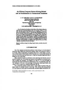
The core of the Northwin tradersD database is a set of 3202 ground facts distributed over eight predicates. This extensional component of the database can be viewed as a relational database (cf. Section 2.5). The schema of this relational database is shown in Figure 2.1. Table 2.1 lists the number of facts for each of the nine predicates in the database. Let us for instance consider the information that is stored on incoming order identi ed by number 10248. Figure 2.2 lists the facts involved. First of all, predicate Order/14 for order 10248 contains: 3

the identi er of the customer, i.e., vinet;

Microsoft and Microsoft Access are registered trademarks by Microsoft, Inc.

28


Figure 2.1: Northwind Traders' relational database schema showing the one-to-many links.

predicate number of facts

Category Customer Employee Order OrderDetail Product Shipper Supplier

8 91 9 830 2155 77 3 29

Table 2.1: Number of facts per predicate in Northwind Traders' database.


29

the identi er of the the Northwin tradersD employee responsible for the transaction, i.e., 5 ;

three important dates: when the order arrived, when the products were due, and when the products were shipped; and

some shipping details: the identi er of the shipping company involved, i.e., 3 , the freight cost, i.e., 32.38, and the six- eld address where to send the products.

Second, predicates Customer/11, Employee/17, and Shipper/3 provide all required details on customer vinet (named Vins et alcools Chevalier), employee 5 (named Steven Buchanan), and shipper 3 (named Federal Shipping). As this customer, employee, and shipper may be involved in many orders, it makes sense to store this information once in separate predicates, rather than repeatedly in the Order predicate. Third, per product ordered in order 10248, predicate OrderDetail/5 contains a fact with:

the identi er of the product, e.g., 11 ; and

some transaction-speci c information on the product: the price paid, the quantity ordered, and the discount granted.

Fourth, general information on the products ordered is stored in predicate Product/10, e.g., for product 11 :

the name of the product, i.e., Queso Cabrales;

the identi er of the supplier of Queso Cabrales, i.e., 5 ;

the identi er of the product category, i.e., 4 ;

some details related to the supply of the product: the quantity per unit, the price of a unit, the number of units in stock and on order, the level of stock at which the product should be reordered, and a boolean value to indicate whether the product is discontinued.

Finally, for each product in order 10248, predicates Category/4 and Supplier/11 contain information on the supplier and the nature of the

product. For instance, product Queso Cabrales (product identi er 11 ) in order 10248 is a diary product (category identi er 4 ) supplied by Cooperativa de Quesos `Las Cabras' (supplier identi er 5 ).

30


Order (10248, vinet, 5, 1 7 93, 29 7 93, 13 7 93, 3, 32.38, vins et alcools Chevalier, 59 rue de l'Abbaye, reims, null, 51100, france) Customer (vinet, vins et alcools Chevalier, paul Henriot, accounting manager, 59 rue de l'Abbaye, reims, null, 51100, france, 26471510, 26471511) Employee (5, buchanan, steven, sales manager, mr., 4 3 55, 17 10 93, 14 Garrett Hill, london, null, sw1 8 jr, uk, 71 555-4848, 3453, image, text, 2) Shipper (3, federal shipping, 503 555-9931) Orderdetail (10248, 11, $14.00, 12, 0.00 ) Orderdetail (10248, 42, $9.80, 10, 0.00 ) Orderdetail (10248, 72, $34.80, 5, 0.00 ) Product (11, queso cabrales, 5, 4, 1 kg pkg., $21.00, 22, 30, 30, 0) Product (42, singaporean fried mee, 20, 5, 32-1 kg pkgs., $14.00, 26, 0, 0, 1) Product (72, mozzarella di giovanni, 14, 4, 24-200 g pkgs., $34.80, 14, 0, 0, 0) Category (4, dairy products, cheeses) Category (5, grains cereals, breads crackers pasta and cereal) Supplier (5, cooperativa de Quesos Las Cabras, antonio del Valle Saavedra, export administrator, calle del Rosal 4, oviedo, asturias, 33007, spain, 98 598-76-54, null) Supplier (14, formaggi Fortini s.r.l., elio Rossi, sales representative, viale dante 75, ravenna, null, 48100, italy, 0544 60323, 0544 60603) Supplier (20, leka trading, chandra Leka, owner, 471 Serangoon Loop Suite#402, singapore,null, 0512, singapore, 555-8787, null)

Figure 2.2: Facts from Northwind Traders' database about order number 10248.


31

2.7.2 Intensional component

A rst type of rules added in the intensional component of the Northwin tradersD database are projection rules. These simply select a few terms from the predicate. For instance, for predicate OrderDetail / 5: OrderDetailID (OrderID,ProductID ) OrderDetail (OrderID,ProductID,UnitPrice,Quantity,Discount) OrderDetailUnitPrice (OrderID,ProductID,UnitPrice) OrderDetail (OrderID,ProductID,UnitPrice,Quantity,Discount) OrderDetailQuantity (OrderID,ProductID,Quantity) OrderDetail (OrderID,ProductID,UnitPrice,Quantity,Discount) OrderDetailDiscount (OrderID,ProductID,Discount) OrderDetail (OrderID,ProductID,UnitPrice,Quantity,Discount)

In a similar fashion, for each of the other seven predicates Pred / n in the extensional database of Section 2.7.1, and for each term Termi (2 i n) in Pred/ n, the following rules are added: PredID (Term1 ) Pred (Term1 ,. . . ,Termn ) PredTermi (Term1 ,Termi ) Pred (Term1 ,. . . ,Termn ) Except in predicate OrderDetail / 5, for which the rules are shown above, Term1 is always the key argument. Throughout the text, we will extend the intensional component of the Northwin tradersD database with additional, less trivial, rules.

32


Chapter 3

Task De nitions 3.1 Introduction Discovery of recurrent patterns in large data collections has become one of the central topics in data mining. In tasks where the goal is to uncover structure in the data and where there is no preset target concept, the discovery of relatively simple but frequently occurring patterns has shown good promise. Association rules (Agrawal, Imielinski, and Swami 1993) are a basic example of this kind of setting. A prototypical application example is in market basket analysis: nd out which items tend to be sold together. The motivation for such an application is the potentially high business value of the discovered patterns. At the heart of the task is the problem of determining all combinations of items that occur frequently together, where \frequent" is de ned as \exceeding a user-speci ed frequency threshold". The use of a frequency threshold for ltering out non-interesting patterns is natural for a large number of data mining problems. Patterns that are rare, e.g., that concern only a couple of customers, are probably not reliable nor useful for the user. See Section 1.2.1, for a more extensive motivation of the frequent pattern discovery task. In this chapter, we consider a formulation in rst-order logic for a large subfamily of this type of tasks. First, in Section 3.2 we recapitulate the generic de nition of frequent pattern discovery and instantiate this de nition to the frequent pattern discovery in logic task. In three subsequent Sections 3.3, 3.4, and 3.5 we specify the notion of frequency for the three pattern classes of interest: queries, query extensions, and clauses. Finally, in Section 3.7, we relate frequent pattern discovery in logic to other approaches 33

34

CHAPTER 3. TASK DEFINITIONS

for induction, especially those in inductive logic programming. In Chapter 4, we discuss two formalisms for the declaration of pattern language L. These formalisms are essential for the exibility of our approach. They allow us to formalize some of the existing variants of the association rule task as special cases. All algorithmic solutions to the problems introduced in this chapter are postponed to Chapter 6.

Bibliographical note

Parts of this chapter have been published before. This introduction, Section 3.2 and Section 3.3 contain excerpts from (Dehaspe and Toivonen, 1998); and Section 3.7 from (De Raedt and Dehaspe, 1997a).

3.2 Frequent pattern discovery in logic A family of data mining problems can be speci ed as follows (Mannila and Toivonen, 1997).

De nition 3.1 Given a database r, a class L of sentences (patterns), and a selection predicate q, the interesting pattern discovery task is to nd the theory of r with respect to L and q, i.e., the set T h(L; r; q) = fQ 2 L j q(r; Q) is trueg: The selection predicate q is used for evaluating whether a sentence Q 2 L de nes a (potentially) interesting pattern in r. 3 For the discovery of frequent patterns, q is de ned so that q(r; Q) is true if and only if the frequency of pattern Q in database r exceeds the fre-

quency threshold. Thus, in terms of the generic formulation of the frequent pattern discovery problem by Heikki Mannila and Hannu Toivonen (1997) of De nition 3.1, we consider the following data mining task.

De nition 3.2 Assume r is a de nite database, and L is a set of queries, a set of query extensions, or a set of clauses. Further assume that each pattern P 2 L contains an atom key, and q(P,r; key) is true if and only if the frequency of pattern P with respect to r given key is at least equal to the frequency threshold speci ed by the user. The frequent pattern discovery in logic task is to nd the set T h(L; r; q; key) of frequent patterns. 3 Notice we have added a new parameter key to the original formulation of Mannila and Toivonen (1997). In our framework this extra parameter is essential, as it determines what is counted. As we will shortly clarify in our de nition of frequency, each binding of the variables in key uniquely identi es an entity. It has been absent from previous formulations of the

3.3. FREQUENT QUERY DISCOVERY

35

task because it has always followed unambiguously from the application context. The original absence of the key parameter can be traced back to the limited knowledge representation framework in which frequent pattern discovery has traditionally been casted. Reconsider the canonical market basket problem. There is no confusion possible about the object of counting: market baskets (also called transactions). Compare this to the Northwin tradersD database in Section 2.7. We can do something similar and count orders. But we might as well focus on customers, or employees, or any of the seven other objects. With the key parameter we can change this focus while leaving the other inputs, in particular database r, untouched. In practice, as already mentioned in De nition 3.2, key takes the form of an atom, for example OrderID (OID ). We can treat this atom as a query and submit it to the database. Each answering substitution k that makes this query true w.r.t. the database uniquely identi es an example ek . For instance, fOID/10248g identi es order 10248. The set of all answering substitutions corresponds to the total set of objects we want to count, i.e., in the example above, there is one unique answering substitution for each of the 830 orders. Since this key atom is an obligatory part of each pattern P in L, we can construct a unique pattern Pk per example ek . For instance, let P be query OrderID (OID ) ^ OrderShipCountry (OID,france), then OrderID (10248) ^ OrderShipCountry (10248,france) is the unique pattern P fOID/10248g that corresponds to example order 10248. We can then count how many of these patterns Pk , 830 in the example above, match the database. The outcome corresponds to the number of examples ek in which pattern P occurs, i.e., the frequency of P . A detailed formal account of the key parameter of De nition 3.2 is given in the three following sections, where we formally de ne what frequency exactly means in the three considered instances of frequent pattern discovery in logic.

3.3 Frequent query discovery With L a set of queries (see De nition 2.13), De nition 3.2 is supplemented with the following de nition of frequency.

De nition 3.3 Assume r is a de nite database and Q 2 L is a query that contains atom key. Then the frequency of query Q with respect to database r given key is frq (Q; r; key ) = jf 2 answerset (key; r) j Q matches rgj jf 2 answerset (key; r)gj

36


i.e., the fraction of substitutions of the key variables with which the query Q is true, or, more intuitively, the fraction of examples in which pattern Q occurs. 3 Example 3.1 Consider the Northwin tradersD database rnw, and assume we look for frequent queries with the focus on orders. If we want to count orders, we have to make sure the key variables equal the rst argument of predicate Order/ 14. Using one of the intensional de nitions described in Section 2.7.2, we set key to atom OrderID (OID ). This has a double eect. First, all patterns contain an obligatory atom OrderID (OID ). The second eect has to do with the computation of frequency. Suppose we want to count the frequency of query Q1 = OrderID (OID ) ^ OrderShipCountry (OID,france) i.e., \an order shipped to France". For each fact of predicate Order/ 14, there is a substitution k = fOID/oidk g 2 answerset (OrderID (OID ), rnw) : For instance, for the fact shown in Figure 2.2, the substitution equals fOID/10248g. As can be seen in Table 2.1, there are in total 830 such substitutions w.r.t. the database, i.e., jf 2 answerset(OrderID (OID ), rnw)gj = 830 We then have to nd the fraction of these substitutions k for which Q1 k = OrderId (oidk ) ^ OrderShipCountry (oidk ,france) is true w.r.t. rnw. As can be observed in Figure 2.2, this query indeed holds for oidk = 10248. As it turns out, the query matches with in total 77 order numbers, i.e., jf 2 answerset(OrderID (OID ), rnw) j Q1 matches rnwgj = 77 From these two numbers, we obtain the nal result: 77 frq (Q1 ; rnw; OrderID (OID ) ) = 830 ' 0:093

To conclude this section, let us once more establish the link with relational database terminology (see also above, Section 2.5). In SQL syntax the absolute frequency of Q with respect to a relational database can be obtained with the following query, inspired by (Lindner and Morik, 1995, Blockeel and De Raedt, 1996):

3.4. FREQUENT QUERY EXTENSION DISCOVERY

37

select count(distinct *) from select elds that correspond to the variables in key from relations in Q where conditions expressed in Q

Example 3.2 We can compute the above frequency (see Example 3.1) frq (OrderID (OID ) ^ OrderShipCountry (OID,france); rnw; OrderID (OID ) ) in SQL, by dividing the result of SQL-query select count(distinct *) from select OrderID.OID from OrderID, OrderShipCountry where OrderID.OID = OrderShipCountry.OID and OrderShipCountry.ShipCountry=`france'

by the total number of orders, i.e., 830.

3.4 Frequent query extension discovery 3.4.1 Frequency

With L a set of query extensions (see De nition 2.14), De nition 3.2 is supplemented with the following de nition of frequency.

De nition 3.4 Assume r is a de nite database and E is a query extension 2 L such that key occurs in the body of E . Then the frequency of query extension E with respect to database r given key is frqe (E; r; key ) = frq (conclusion (E ); r; key ) i.e., the fraction of substitutions of the key variables with which the conclusion of E is true, or the fraction of examples in which pattern E non-trivially holds1 . 3

Example 3.3 Let us continue Example 3.1. Suppose we add to rnw 15 facts EUmember (austria) , . . . , EUmember (uk) for the currently 15 1 The pattern trivially holds if the body does not match the database. These cases are excluded: if the conclusion of a query extension holds, so does its body.


38

member states of the European Union, and compute the frequency of an extension of query Q1 that looks as follows:

E1 = OrderID (OID ) ^ OrderShipCountry (OID,france) ;

OrderDetailID (OID,PID ) ^ ProductSupplierID (PID,SID ) ^ SupplierCountry (SID,SC ) ^ EUmember (SC )

i.e., \if an order OID is shipped to France, then there is a product PID in the order which is supplied by a company SID from a member state SC of the European Union". The conclusion of E1 is

Q2 = OrderID (OID ) ^ OrderShipCountry (OID,france) ^


For instance, the facts in Figure 2.2 reveal that the query Q2 is true with substitution fOID/10248, PID/11, SID/5, SC /spaing. For the full Northwin tradersD database we obtain: frqe (E1 ; rnw; OrderID (OID ) ) = frq (Q2 ; rnw; OrderID (OID ) ) 55 ' 0:066 = 830

3.4.2 Con dence

As discussed in Section 2.3, query extensions descend from association rules. Apart from frequency, association rules have traditionally been labeled with a second quality criterion, namely con dence (Agrawal, Imielinski, and Swami 1993). We now upgrade the notion of con dence to the case of query extensions.

De nition 3.5 As before, assume r is a de nite database and E is a query extension 2 L such that key occurs in the body of E . Then the con dence of query extension E with respect to database r given key is confqe (E; r; key ) =

frqe (E; r; key ) = frq (conclusion (E ); r; key ) frq (body (E ); r; key ) frq (body (E ); r; key )

i.e., the ratio of the frequencies of conclusion and body of E , or the share of examples matched by the body that are also matched by the conclusion of E . 3


39

Example 3.4 Recall queries Q1 = OrderID (OID ) ^ OrderShipCountry (OID,france) Q2 = OrderID (OID ) ^ OrderShipCountry (OID,france) ^


and query extension

E1 = OrderID (OID ) ^ OrderShipCountry (OID,france) ;


Then, the combination of the results from Examples 3.1 and 3.3 gives: frq (Q ; rnw; OrderID (OID ) ) confqe (E1 ; rnw; OrderID (OID ) ) = frq (Q2; rnw; OrderID(OID) ) 1 55 = 77 ' 0:71 This outcome should be interpreted as: \71% of the orders that go to France contain a product supplied by a EU-based company".

3.4.3 Deviation

We will use a third quality criterion for query extensions which is less common in the association rule literature: the deviation label on a query extension indicates the unusualness of the dependency between the body and the conclusion. Example 3.5 It is not clear from Example 3.4 whether there is anything special about the orders shipped to France. It might well be that, overall, about three quarters of the orders in the Northwin tradersD database contain EUsupplied products. In that case, the rule in Example 3.4 may not be worth noticing2 , orders to France behave just as expected. If on the other hand on average as much as 98% or as few as 45% of the orders turn out to contain EU-supplied products, orders to France seem to deviate from the expected as they contain unusually less or more of such products3 . 2 A dierence of say 71%-75% may still be \important" if the number of observed orders is very large. Our deviation measure should (and will) account for this. 3 The inverse of the previous comment holds here. If only say ten orders are observed, even a dierence 71%-98% may be nonessential.


40

Various deviation measures have been proposed in a data mining context, e.g., in Explora (Klosgen, 1992, Klosgen, 1996) and Midos (Wrobel, 1997). We use the binomial distribution to measure the deviation of the con dence of a rule from the mean.

De nition 3.6 Assume an experiment that consists of N trials, where in each trial some event either happens or fails to happen. Let p be the probability that the event will happen in a single trial, and q = 1 ? p be the probability that the event will fail to happen in a single trial. We can then compute the probability that the event will happen in exactly X trials (and fail to happen in N ? X trials) with the following probability function:

bino (p; N; X ) =

P

N X

pX qN ?X

Since NX =0 bino (p; N; X ) = 1, function bino de nes a discrete probability distribution, called the binomial distribution (or Bernoulli distribution) for X. Given N and P p, the probability that an event will happen in Y or more trials is NX =Y bino (p; N; X ). If Y is greater then mean pN , this probability is less than 0.5, and weP say result Y deviates positively from mean pN . The closer probability NX =Y bino (p; N; X ) approaches 0, the higher the positive deviation. GivenPN and p, the probability that an event will happen in Y or less trials is YX =0 bino (p; N; X ). If Y is less then mean pN , this probability is less than 0.5, and wePsay result Y deviates negatively from mean pN . The closer probability YX =0 bino (p; N; X ) approaches 0, the higher the negative deviation. 3 We now translate these de nitions to the present context. The experiment consists in repeatedly drawing an object matched by the body of the clause, where N is the absolute frequency of the body. Following (Klosgen, 1992, Klosgen, 1996), we call this set the subgroup. In Example 3.5 the subgroup would be the orders shipped to France, and since there are 77 of these, N = 77. Again following (Klosgen, 1992, Klosgen, 1996), we call the set of objects matched by the head of the query extension the target group. Each time we draw an element from the subgroup, this element can either be in or out the target group. The probability p that event \in target group" will happen in a single trial \draw from subgroup" is assumed to be identical to the probability that event \in target group" will happen in a single trial \draw from total population". That is, p is set to the frequency of the head


41

of the query extension. In Example 3.5 this is the fraction of orders that contain EU-supplied products, which happens to be 0.79. We then observe the result of the experiment. The number of successful trials corresponds to the number of elements in the intersection of subgroup and target group, in other words, to the absolute frequency of the query extension. In Example 3.5, there are 55 orders that are shipped to France and contain EU-supplied products. Finally, we can compare the outcome of the experiment with the assumed mean and measure to what extent it deviates (positively or negatively). In Example 3.5, we expect 0:7977 ' 61 elements in the intersection. Obviously, our observed result 55 deviates negatively. We quantify this deviation as follows: if we draw 77 elements from the set of all orders, then the probability thatP this selection will contain 55 or less orders with a EUsupplied product is 55 X =0 bino (0:79; 77; X ) ' 0:07. This means that, if we repeat the experiments 100 times, a result of 55 or less is bound to come up in about 7 cases. For comparison, a result of 49 or less will only occur in one out of a thousand experiments, 42 or less in on out of a million experiments, and we need 1020 experiments to encounter a case where the result is 23 or less. In Example 3.5, a subgroup of 77 orders where only 23 contain EU-supplied products would be a lot more unusual than the subgroup of orders shipped to France that we have considered. It should be stressed at this point that it is necessary to be very careful with any statistical interpretation of the deviation test. In statistical decision theory, the 0:07 would be interpreted as the signi cance level of the hypothesis that the proportion of target group elements diers in the subgroup and the total population. We have warned against such interpretation before in Section 1.2.2 (\It's just (unorthodox) statistics!"). The problem is that in frequent query discovery we look at many target groups. Due to what statisticians call the multiplicity eect (Salzberg, 1997), some of them are bound to come up seemingly \signi cant". Therefore we use the deviation measure rather as a ranking criterion. Its purpose is to lter away uninteresting patterns, rather than to corroborate interesting ones. The closer the deviation is to 0.5 the less interesting it is. We now provide a more formal de nition the deviation of query extensions: De nition 3.7 As before, assume r is a de nite database and E is a query extension 2 L such that key occurs in the body of E . Furthermore, let

E 0 = key ^ head (E ); with E 0 range-restricted p = frq (E 0 ; r; key ) N = jf 2 answerset (key; r) j body (E ) matches rgj


42

Y =

jf 2 answerset (key; r) j conclusion (E )

matches rgj

Then the positive deviation of query extension E with respect to database r given key is pdevqe (E; r; key ) =

N X

X =Y

bino (p; N; X ) ;

the negative deviation of query extension E with respect to database r given key is ndevqe (E; r; key ) =

Y X

X =0

bino (p; N; X ) ;

and the deviation of query extension E with respect to database r given key is devqe (E; r; key ) = minimum (pdevqe (E; r; key ); ndevqe (E; r; key )) :

3

Example 3.6 Consider again Examples 3.3-3.5. We have already computed the negative deviation of query extension E1 : ndevqe (E1 ; rnw; OrderID (OID ) ) =

55 X

X =0

bino (0:79; 77; X ) ' 0:07

If we combine this with the positive deviation of query extension E1 pdevqe (E1 ; rnw; OrderID (OID ) ) =

77 X

X =55

bino (0:79; 77; X ) ' 0:96

we nd4 devqe (E1 ; rnw; OrderID (OID ) ) ' minimum (0:96; 0:07) = 0:07

P

bino (0:79; 77; X ) = 1, the sum of the negative and posObserve that, while 77 X =0 itive deviation is greater than one. This is caused that bino (0:79; 77; 55) P bybinothe(0:fact 79 ; 77 ; X ) ' 0:04, which is is counted twice. Notice in that respect that 54 X =0 equal to one minus positive deviation 0.96. 4

3.5. FREQUENT CLAUSE DISCOVERY

43

3.5 Frequent clause discovery 3.5.1 Frequency

Finally, with L a set of de nite clauses (see De nition 2.11), De nition 3.2 is supplemented with the following de nition of frequency.

De nition 3.8 Assume r is a de nite database and C is a de nite clause occurs in body(C ). Then the frequency of clause C with respect to database r given key is frc (C; r; key ) = frq (body (C ); r; key ) ? frq (body (C ) ^ :head (C ); r; key )

2 L, such that key

i.e., the fraction of substitutions of the key variables with which both query body(C ) and clause C are true, or the fraction of examples in which pattern C non-trivially holds. 3

Example 3.7 Let us, for a change, count customers in the Northwin tradersD database rnw and set key to CustomerID (CID ). We also enrich the intensional part of rnw with the following de nitions: CustomerEUmember (CID ) CustomerID (CID ) ^ CustomerCountry (CID,Country) ^ EUmember (Country)

to test whether a customer lives in a EU country, and ProductCheap (PID)

ProductUnitPrice (PID,Price) ^ Price < $55

to test whether a product is cheap in the sense that its price is below $55. Consider the following clause:

C1 = ProductCheap (PID )

CustomerID (CID ) ^ CustomerEUmember (CID ) ^ OrderCustomerID (OID,CID ) ^ OrderDetailID (OID,PID )

i.e., \if a customer CID is a EU citizen and places an order OID that contains a product PID then that product PID is cheap", in other words, the customer orders only cheap things. The body of C1 matches 48 out of 91 customers in the database: the remaining 43 customers either have their address outside the EU or have not placed any orders. From these 48, we have to subtract the examples where B ^ :H is true w.r.t. rnw. That is, we have to remove the customers who have ordered


44

a product which is not cheap. Afterwards, we are left with the customers who have an exclusive preference for cheap things. Consider the Figure 2.2 facts. The body of C1 is true for customer vinet, for instance, with answering substitution fCID/vinet, OID/10248, PID/11g. This substitution also makes the head of C1 true: the price of product 11 is $21.00 which is indeed less than the $55 threshold. Also the two other products in order 10248 are cheap: product 42 costs $14.00, and product 72 costs $34.80. Apart from order 10248, there are four other orders in the database for customer vinet. It turns out that all of these, like order 10248, only contain cheap products. In other words, customer vinet has not ordered a product which is not cheap and should not be removed from the set of 48 customers matched by the body of C1 . Inspection of the full set of 48 customers reveals that 40 of them, in contrast to vinet, have ordered something cheap on at least one occasion. These correspond to the 40 bindings of CID for which the body of C1 is true, as well as the following query equal to body (C1 ) ^ :head (C1 ): CustomerID (CID ) ^ CustomerEUmember (CID ) ^ OrderCustomerID (OID,CID ) ^ OrderDetailID (OID,PID ) ^ :ProductCheap (PID )

Hence

frc (C1 ; rnw; CustomerID (CID ) ) = 48 ? 40 = 8 ' 0:09 91 91 91 i.e., \about 9% of the customers live in the EU and order exclusively cheap things". At this point, we again draw the reader's attention to the dierence between clauses and query extensions. Query extension CustomerID (CID ) ^ CustomerEUmember (CID ) ^ OrderCustomerID (OID,CID ) ^ OrderDetailID (OID,PID ) ; ProductCheap (PID )

looks similar to clause C1 but holds for EU-customers that have ordered at least one cheap product, rather than only cheap products. It turns out there are 48 customers for which the query extension above holds. As we have seen, only eight of these are also matched by C1 .

3.5.2 Con dence

As we did for query extensions above, we also introduce a second evaluation function that measures the accuracy of the pattern.

3.5. FREQUENT CLAUSE DISCOVERY

45

De nition 3.9 As before, assume r is a de nite database and C is a de nite clause 2 L, such that key occurs in the body of C . Then the con dence of clause C with respect to database r given key is confc (C; r; key ) = frc (C; r; key ) frq (body (C ); r; key ) i.e., the ratio of the frequencies of clause C and query body (C ). 3 Example 3.8 The con dence of clause C1 (see Example 3.7) C1 = ProductCheap (PID ) CustomerID (CID ) ^ CustomerEUmember (CID ) ^ OrderCustomerID (OID,CID ) ^ OrderDetailID (OID,PID ) then equals: confc (C1 ; rnw; CustomerID (CID ) ) (C1 ; rnw; CustomerID (CID ) ) = frq (frc body (C1 ); rnw; CustomerID (CID ) ) 8 = 48 ' 0:17 i.e., \roughly 17% of the EU-customers have ordered exclusively cheap things". Once more, compare the con dence of clause C1 to the con dence of query extension CustomerID (CID ) ^ CustomerEUmember (CID ) ^ OrderCustomerID (OID,CID ) ^ OrderDetailID (OID,PID ) ; ProductCheap (PID ) which is equal to one, i.e., \all EU-customers have ordered at least one cheap thing".

3.5.3 Deviation

Finally, we adapt the deviation of query extensions explained in Section 3.4.3 to clauses. De nition 3.10 As before, assume r is a de nite database and C is a de nite clause 2 L such that key occurs in the body of C . Furthermore, let C 0 = head (C ) key; with C 0 range-restricted p = frc (C 0 ; r; key ) N = jf 2 answerset (key; r) j body (C ) matches rgj Y = frc (C; r; key ) jf 2 answerset (key; r)gj


46

Then the positive deviation of clause C with respect to database r given key is pdevc (C; r; key ) =

N X

X =Y

bino (p; N; X ) ;

the negative deviation of clause C with respect to database r given key is ndevc (C; r; key ) =

Y X

X =0

bino (p; N; X ) ;

and the deviation of clause C with respect to database r given key is devc (C; r; key ) = minimum (pdevc (C; r; key ); ndevc (C; r; key )) :

3

Example 3.9 The deviation of clause C1 of Example 3.7 is not de ned

since C 0 = ProductCheap (PID ) CustomerID (CID ) is not rangerestricted. Therefore, let us change key back to OrderID (OID ) and consider the following clause: C2 = OrderShipCountry (OID,france) OrderID (OID ) ^ OrderDetailID (OID,PID ) ^ ProductSupplierID (PID,SID ) ^ SupplierCountry (SID,france) i.e., \if there is a product PID in the order OID which is supplied by a French company, then the order OID is shipped to France. For C2 , we can assign the following values to the parameters in the deviation formula: C20 = OrderShipCountry (OID,france) OrderID (OID ) 77 ' 0:093 p = frc (C20 ; rnw; OrderID (OID ) ) = 830 N = jf 2 answerset (OrderID (OID ); rnw) j body (C ) matches rnwgj = 167 Y = frc (C; rnw; OrderID (OID ) ) jf 2 answerset (OrderID (OID ); rnw)gj = 6 Then pdevc (C2 ; rnw; OrderID (OID ) ) = ndevc (C2 ; rnw; OrderID (OID ) ) =

167 X

X =6 6 X X =0

bino (0:093; 167; X ) ' 0:999 bino (0:093; 167; X ) ' 0:004

devc (C2 ; rnw; OrderID (OID ) ) = 0:004

3.6. MAPPING QUERY EXTENSIONS TO CLAUSES

47

i.e., in the subgroup of orders that contain France-supplied product, there are less orders shipped to France than expected from the statistics of the total group. If we would randomly select 167 orders from that total group, only in four out of thousand experiments that selection would contain six or less orders shipped to France.

3.6 Mapping query extensions to clauses In Section 2.3 we have argued that clauses and query extensions are so similar { they are both implications { that introduction of new terminology and new notation (;) is justi ed in order to avoid confusion. In this section we relate both patterns in terms of their evaluation functions de ned in the preceding sections. The rst property relates the frequency of query extensions to that of clauses.

Proposition 3.1 frc (H

B; r; key ) + frqe (B ; :H; r; key ) = frq (B; r; key )

3

Proof frc (H

B; r; key ) Def.=3.8 frq (B; r; key ) ? frq (B ^ :H; r; key ) Def.=3.4 frq (B; r; key ) ? frqe (B ; :H; r; key )

2

Example 3.10 Reconsider clause C1 introduced in Example 3.7 C1 = ProductCheap (PID )


and further assume

E2 = CustomerID (CID ) ^ CustomerEUmember (CID ) ^

OrderCustomerID (OID,CID ) ^ OrderDetailID (OID,PID ) ; : ProductCheap (PID ) = body (C1 ) ; :head (C1 )


48 Then

frqe (E2 ; rnw; CustomerID (CID ) ) = frq (body (C1 ); rnw; CustomerID (CID ) ) ? frc (C1 ; rnw; CustomerID (CID ) ) 48 ? 8 = 40 ' 0:44 = 91 91 91 i.e., \about 44% of the customers live in the EU and have ordered at least one product which is not cheap". The following property relates the con dence of clauses and query extensions to each other.

Proposition 3.2

confc (H

B; r; key ) + confqe (B ; :H; r; key ) = 1

3

Proof confc (H

(H B; r; key ) B; r; key ) Def.=3.9 frc frq (B; r; key ) Def.=3.8 frq (B; r; key ) ? frq (B ^ :H; r; key ) frq (B; r; key ) B ^ :H; r; key ) = 1 ? frq (frq (B; r; key ) Def.=3.5 1 ? confqe (B ; :H; r; key )

2

Example 3.11 Using Proposition 3.2, we can obtain the con dence of query extension E2 (see Example 3.10)

E2 = CustomerID (CID ) ^ CustomerEUmember (CID ) ^

OrderCustomerID (OID,CID ) ^ OrderDetailID (OID,PID ) ; : ProductCheap (PID )

from the con dence of clause C1 (see Example 3.8)

C1 = ProductCheap (PID )



49

as follows: confqe (E2 ; rnw; CustomerID (CID ) ) = 1 ? confc (C1 ; rnw; CustomerID (CID ) ) 8 = 40 ' 0:83 = 1 ? 48 48 i.e., \83% of the customers who live in the EU, have ordered at least one cheap product". Finally, we clarify the correspondence between the deviation of query extensions and clauses.

Proposition 3.3 If the head of a query extension and a clause consists of a single literal lh , and lh

key is range-restricted5 then

devqe (B ; lh ; r; key ) = devc (lh

B; r; key )

3

Proof Since both for query extensions and clauses deviation is de ned

as the minimum of positive and negative deviation (see De nitions 3.7 and 3.10), we have to prove that and Let

pdevqe (B ; lh ; r; key ) = pdevc (lh

B; r; key )

ndevqe (B ; lh ; r; key ) = ndevc (lh

B; r; key )

pdevqe (B ; lh ; r; key ) = pdevc (lh

B; r; key ) =

ndevqe (B ; lh ; r; key ) = ndevc (lh

5

If lh

B; r; key ) =

Nq X X =Yq Nc X X =Yc Yq X X =0 Yc X

bino (pq ; Nq ; X ) bino (pc; Nc; X )

bino (pq ; Nq ; X )

bino (pc; Nc ; X ) X =0 key is not range-restricted, the deviation function is not de ned.


50

then it suces to prove the three equations Nq = Nc , pq = pc , and Yq = Yc . First, N Def.=3.7 jf 2 answerset (key; r) j B matches rgj q

Def.=3.10 N c

Second,

pq Def.=3.7 frq (key ^ lh; r; key ) Def.=3.3 jf 2 answerset (key; r) j lh matches rgj jf 2 answerset (key; r)gj jf 2 answerset (key; r) j :lh matches rgj = 1? jf 2 answerset (key; r)gj Def.=3.3 1 ? frq (key ^ :l ; r; key ) h = frq (key; r; key ) ? frq (key ^ :lh ; r; key ) Def.=3.8 frc (l h key; r; key ) Def.=3.10 p c Third,

Yq Def.=3.7 = =

jf 2 answerset (key; r) j (B ^ lh ) matches rgj jf 2 answerset (key; r) j (B ^ :(B ^ :lh )) matches rgj jf 2 answerset (key; r) j B matches rgj ? jf 2 answerset (key; r) j (B ^ :lh ) matches rgj

Def.=3.3 (frq (B; r; key ) ? frq (B ^ :l ; r; key )) h jf 2 answerset (key; r)gj Def.=3.8 frc (l B; r; key ) jf 2 answerset (key; r)gj

Def.=3.10 Y c

h

Example 3.12 Assume query extension E3 = OrderID (OID ) ^ OrderDetailID (OID,PID ) ^

2

ProductSupplierID (PID,SID ) ^ SupplierCountry (SID,france) ; OrderShipCountry (OID,france)


51

and recall clause C2 (see Example 3.9) C2 = OrderShipCountry (OID,france) OrderID (OID ) ^ OrderDetailID (OID,PID ) ^ ProductSupplierID (PID,SID ) ^ SupplierCountry (SID,france) We can then recycle the computations of Example 3.9 to nd devqe (E3 ; rnw; OrderID (OID ) ) = devc (C2 ; rnw; OrderID (OID ) ) ' 0:004

Proposition 3.3 suggests a close correspondence between query extensions and clauses. Propositions 3.1 and 3.2 on the other hand corroborate our earlier observation that, in general, it is dangerous to confuse query extensions and clauses. To round o our discussion of the relationship between these two patterns, we now clarify under which conditions query extensions and clauses can be confused. Under these circumstances not only deviation but also frequency and con dence is identical for query extensions and clauses. Theorem 3.1 Assume a de nite database r, a literal lh, a clause lh B, and a query extension B ; lh . If for all substitutions 2 answerset (key; r), there exists at most one substitution of the variables of lh that makes B true w.r.t. r, then frc (lh B; r; key ) = frqe (B ; lh ; r; key ) confc (lh B; r; key ) = confqe (B ; lh; r; key ) devc (lh B; r; key ) = devqe (B ; lh ; r; key )

3

Proof We refer to Proposition 3.3 for a discussion of the deviation func-

tion, and now concentrate on frequency and con dence. From the condition in Theorem 3.1 it follows that in case B matches r, either (B ^ lh) or (B ^ :lh ) matches r, but not both. Therefore, jf 2 answerset (key; r) j B matches rgj = jf 2 answerset (key; r) j (B ^ lh) matches rgj + jf 2 answerset (key; r) j (B ^ :lh ) matches rgj Def.)3.3 frq (B; r; key ) = frq (B ^ l ; r; key ) + frq (B ^ :l ; r; key ) h h ) frq (B; r; key ) ? frq (B ^ :lh ; r; key ) = frq (B ^ lh ; r; key ) Defs. ) 3.4,3.8 frc (l h B; r; key ) = frqe (B ; lh ; r; key ) Defs. ) 3.5,3.9 confc (l h B; r; key ) = confqe (B ; lh ; r; key )

2

52


Example 3.13 Let us focus on employees (key = EmployeeID (EID )) in the Northwin tradersD database and rst consider a case where the conditions of Theorem 3.1 are not met. B1 = EmployeeID (EID ) ^ EmployeeCountry (EID,SC ) ^

OrderEmployeeID (OID,EID ) lh1 = OrderShipCountry (OID,SC ) Consider the two variables in lh1 (i.e., OID and SC ), and the Figure 2.2 facts. With EID = 5, there is a single binding SC /uk that makes B1 true. This is not the case for OID. Although Figure 2.2 only shows OID/10248, there are in the database 42 such bindings, i.e., employee 5 has been responsible for 42 orders. The order shown in Figure 2.2 comes from France, but others come from the United Kingdom. In fact, all employees have dealt with an order shipped to their own country, but never exclusively. Hence, frqe (B1 ; lh1 ; rnw; EmployeeID (EID ) ) = confqe (B1 ; lh1 ; rnw; EmployeeID (EID ) ) = 1 frc (lh1 B1 ; rnw; EmployeeID (EID ) ) = confc (lh1 B1 ; rnw; EmployeeID (EID ) ) = 0

If, on the other hand, we count orders (key = OrderID (OID )) and assume

B2 = OrderID (OID ) ^ OrderShipCountry (OID,SC ) ^

OrderEmployeeID (OID,EID ) lh2 = EmployeeCountry (EID,SC ) then the conditions of Theorem 3.1 are met. Once OID is xed, there is only one binding of variables EID and SC that makes B2 true. As shown in Figure 2.2, for order 10248 this unique substitution is fEID/5, SC /ukg. Because frq (B2 ; rnw; OrderID (OID ) ) = 1 we obtain: frqe (B2 ; lh2 ; rnw; OrderID (OID ) ) = frc (lh2 B2 ; rnw; OrderID (OID ) ) = confqe (B2 ; lh2 ; rnw; OrderID (OID ) ) = confc (lh2 B2 ; rnw; OrderID (OID ) ) 108 ' 0:13 = 830

3.7. RELATED PROBLEM SETTINGS

53

Strictly speaking, query extension B2 ; lh2 should be read as follows: \if for a given order OID a country SC exists to which the order is shipped, and an employee EID exists who has handled the order, then a country SC exists to which the order is shipped, and an employee EID exists who has handled the order, where employee EID lives in country SC". On the other hand, the correct reading of clause lh2 B2 is \if an order OID is shipped to country SC and handled by an employee EID, then employee EID lives in country SC". Since in this case the conditions speci ed in Theorem 3.1 are met, we can consider these two readings to be equivalent.

3.7 Related problem settings In the previous sections we have already cast our discovery task as instances of the pattern discovery setting by by Mannila and Toivonen (1997) (see De nition 3.1). In this section we point out relations to other frameworks for discovery.

3.7.1 Inductive logic programming Given our use of clausal logic for the representation of data and patterns, we can situate our setting within the eld of inductive logic programming, though not at the center of that eld. Below, in Sections 3.7.5 and 3.7.6, we give two argument for the atypical nature of our approach. Inductive logic programming is a subarea of machine learning. Steve Muggleton named and de ned the eld in 1990 (Muggleton, 1990), but, as usual, there is a lot of research highly relevant to inductive logic programming which dates back to the period before the name was invented. For instance, the work by Plotkin (Plotkin, 1970, Plotkin, 1971) and Shapiro (Shapiro, 1983) is foundational to many current inductive logic programming systems. Textbooks on inductive logic programming include (Muggleton, 1992, Lavrac and Dzeroski, 1994, Bergadano and Gunetti, 1995, De Raedt, 1996, Nienhuys-Cheng and Wolf, 1997, Lavrac and Dzeroski, 1998). For an overview of inductive logic programming work in the context of knowledge discovery in databases, we refer to (Dzeroski, 1996). In the following chapters, where we build up towards algorithms for solving the tasks introduced in this chapter, we will heavily rely on the theoretical and methodological achievements of the still very active inductive logic programming eld.


54

3.7.2 Learning from interpretations

Our de nitions of evaluation functions (see Sections 3.3-3.5) are rooted in the learning from interpretations paradigm, introduced by De Raedt and Dzeroski (De Raedt and Dzeroski, 1994) and related to other settings in (De Raedt, 1997). Let us consider De nition 3.3 of the frequency of queries: frq (Q; r; key ) = jf 2 answerset (key; r) j Q matches rgj jf 2 answerset (key; r)gj In this de nition the varying query Q is matched against a constant database r. Alternatively, we can vary the database and match a xed query Q against rk . Instead of r, we would then have a set of rk 's as input parameter to frq. De nition 3.11 Assume R = fr1; : : : ; rng is a set of de nite databases and Q 2 L is a query. Then the frequency of query Q with respect to R is jfr 2 R j Q matches rk gj frq (Q; R) = k

n i.e., the fraction of databases that query Q matches.

3

Each rk can be viewed as an interpretation ik of rk (more speci cally, ik is the minimal Herbrand model of rk , cf. Section 2.4.1). From that perspective we would indeed be learning from interpretations ik , cf. (De Raedt and Dzeroski, 1994). A straightforward mapping exists from R to r and from Q to Q0 such that frq(Q; R) = frq (Q0 ; r; key ). Basically, we have to

add atom key to Q, add the variables in key as extra arguments to each of the literals in Q, and set Q0 to the modi ed Q0 ; and associate each database rk in R with a unique ground instance of the key variables, and add these constants as extra arguments to each of the literals in rk , and set r to the union of the modi ed rk 's. Example 3.14 Assume Rmail is a set of databases that each contain data about a dierent mail-order company. They are all built according to the relational database schema of Figure 2.1, and one of them is our familiar Northwin tradersD database rnw. Reconsider query Q2 introduced in Example 3.3:




55

Using De nition 3.11, we can then compute frq (Q2 ; Rmail ) as the fraction of mail-order companies that have shipped an order with a EU-supplied product to France. Company Northwin tradersD is in that fraction: the sample data of Figure 2.2 show that query Q2 matches rnw with substitution fOID/10248, PID/11, SID/5, SC /spaing. Let us now apply the mapping as described above: we set key to CompanyID (C ) and construct a pair (Q02 ; rmail ) such that frq (Q2 ; Rmail ) = frq (Q02 ; rmail ; CompanyID (C ) ). First, we add CompanyID (C ) to Q2, and the company identi er C to all literals in Q2 :

Q02 = CompanyID (C ) ^

OrderID (C,OID ) ^ OrderShipCountry (C,OID,france) ^ OrderDetailID (C,OID,PID ) ^ ProductSupplierID (C,PID,SID ) ^ SupplierCountry (C,SID,SC ) ^ EUmember (C,SC )

Second we assign a unique label to each company, and add this label as an extra argument to each predicate. For instance, we might assign label nw to company Northwin tradersD and modify rnw as illustrated below, with a fact for the key predicate, four facts from Figure 2.2, and a clause from Section 2.7.2. CompanyID (nw) Shipper (nw, 3, federal shipping, 503 555-9931) OrderDetail (nw, 10248, 11, $14.00, 12, 0.00 ) Product (nw, 11, queso cabrales, 5, 4, 1 kg pkg., $21.00, 22, 30, 30, 0 ) Category (nw, 4, dairy products, cheeses) OrderDetailID (C,OrderID,ProductID ) OrderDetail (C,OrderID,ProductID,UnitPrice,Quantity,Discount) The data for all companies is then combined into rmail , and we are ready to compute frq (Q02 ; rmail ; CompanyID (C ) ) using De nition 3.3. Observe that with = fC=nwg, Q02 matches rmail with substitution fOID/10248, PID/11, SID/5, SC /spaing, as before.

Notice that in De nition 3.11 the key parameter is not used. Recall this parameter is needed to determine the objects to be counted. The learning from interpretations paradigm however starts from a dataset which is already split into entities to count. In that sense, our formulation of the frequent query discovery task in De nition 3.3 is more general and enables a greater exibility than the one in De nition 3.11. On the other hand, the original formulation in terms of interpretations does make two advantages of this framework better visible.

56


First, from a more theoretical perspective, the learning from interpretations framework links our setting to traditional settings based on propositional logic. For instance, in the canonical market basket application of frequent pattern discovery, examples (transactions) are represented as a set of items. Such an item set corresponds to an interpretation in our setting. A common characteristic of this representation is that all examples are assumed to be completely speci ed: an item not present in the transaction is assumed to be absent. A consequence of this link with propositional approaches is that theoretical results carry over, cf., e.g., the PAC-learning results of (De Raedt and Dzeroski, 1994), and so do popular attribute-value learning techniques. Apart from the systems discussed in this dissertation, a whole sequence of upgrades to rst-order logic have been realized (De Raedt et al., 1998): CN2 (Clark and Niblett, 1989)-ICL (De Raedt and Van Laer, 1995), C5.0 (Quinlan, 1993)-Tilde (Blockeel and De Raedt, 1998), hierarchical clustering (Langley, 1996)-(Blockeel, De Raedt, and Ramon 1998), and reinforcement learning (Dzeroski, De Raedt, and Blockeel 1998). Secondly, a practical advantage follows from the fact that matching a pattern against a smaller database rk is more ecient than matching that same pattern against the full r. We come back to the topic of eciency in Chapter 6, where we discuss algorithms for frequent pattern discovery in logic.

3.7.3 Michalski's, Helft's and Flach's settings The learning from interpretations paradigm as formalized here, can be regarded as a logical formalization of the task addressed by Michalski's Induce system (Michalski, 1983). The advantages of this formalization include: rst, the de nitions inherit from logic their clear and well understood meaning; and second, the integration (and implementation) of background knowledge is very natural. De Raedt and Dzeroski's (1994) setting for discovery is derived from Nicolas Helft's non-monotonic semantics for induction (Helft, 1989). Although it diers from Helft's setting in several respects, both settings share two basic ideas. First, all examples are completely speci ed. Second, patterns that match an example are true w.r.t. that example. Peter Flach's (Flach, 1995) adequacy conditions for induction provide a framework for reasoning about the properties and semantics of induction. However, Flach's adequacy conditions allow for many instantiations. Our framework can be considered one such instantiation, which is close to Flach's con rmatory setting.


57

3.7.4 Clausal Discovery Chapter 6 discusses the Claudien system (De Raedt and Bruynooghe, 1993, De Raedt and Dehaspe, 1997a) for nding frequent clauses. Other systems that handle the discovery of interesting clauses are Knowledge Miner (Shen et al., 1996), Midos (Wrobel, 1997), RDT (Kietz and Wrobel, 1992), Mobal (Lindner and Morik, 1995), Laurel (Weber, 1997, Weber, 1998), and Progol in learning from positive examples only mode (Muggleton, 1996). Apart from Claudien, the setting that is closest to our framework is that of Midos. Midos concerns the multi-relational discovery of subgroups. The subgroups de ned in (Wrobel, 1997) correspond to queries. Midos also employs the notion of a key to count the coverage or of a subgroup (= query). What we call key is called the object relation or master relation in (Wrobel, 1997). With K the variables in the object relation (= key), the coverage of a subgroup (= query) is de ned as follows (Wrobel, 1997): c(Q) := K (f j Q matches rg) ; where K denotes the projection onto variables K . In words, the coverage c(Q) of a subgroup Q is de ned as the set of bindings of the variables in the object relation for which query Q matches the database. We use an equivalent expression in our de nition of frequency of a query. Recall the nominator of the fraction in De nition 3.3: f 2 answerset (key; r) j Q

matches rg

i.e., \the examples in the database that are covered by query Q". We only have to take the cardinality of c(Q) and divide it by the number of examples in the database to arrive at our notion of relative frequency of Q. This observation leads us to conclude that Midos, like our setting (see Section 3.7.2) also ts in the learning from interpretations framework. This is not surprising given the fact that Midos, like our setting, can be considered an upgrade to rst-order logic of a propositional system, in this case Explora (Klosgen, 1992, Klosgen, 1996). What distinguishes Midos from our setting is that Midos is tailored towards a single quality criterion which is not frequency but \distributional unusualness with respect to a certain property of interest" (Wrobel, 1997). More speci cally, Midos solves the task of nding in a language of queries the n most unusual ones6 . 6

One could say Midos more or less relates to our our setting like Explora relates to

Apriori.

58


The \unusualness" measure which is used corresponds to deviation in our setting. The \property of interest" can, at least in some cases, be encoded as the head of a clause (where the subgroup corresponds to the body of the clause). Thus, roughly stated in our terminology, Midos solves the task of nding in a language of clauses L, the n clauses with highest deviation. To solve this task in an ecient way, Midos uses optimistic estimate pruning techniques and an optimal re nement operator. We refer to (Wrobel, 1997) for more details.

3.7.5 Concept learning In our descriptive setting, the goal is to nd individual useful patterns in a database that is viewed as a monolithic entity. In machine learning in general and inductive logic programming in particular, people have classically focused on learning patterns that in combination with each other discriminate between dierent classes {typically positive examples and negative examples{ within the database. This has been called the classi cation or concept learning task. The intention is to use the induced set of patterns to predict the class of new examples, i.e., examples for which no class value is known. To adapt our current setting to concept learning, we should rst partition the examples into a number of classes. For simplicity, we assume two classes and . Recall that, for instance in De nition 3.3, the set of examples is represented by the set of substitutions f 2 answerset (key; r)g. A partition on this set would result in \classi ed substitutions", where a class label or is assigned to each substitution: denotes a substitution that corresponds to a positive example and denotes a substitution that corresponds to a negative example. The concept learning task is then to nd a set of patterns H L such that for any \positive substitution" , H matches r (the completeness requirement), and for any \negative substitution" , H does not match r (the consistency requirement).

Example 3.15 With key equal to CustomerID (CID ), we have 91 examples in the database, one for each 2 answerset (CustomerID (CID ),rnw) = fCID/alfki, . . . , CID/wolzag; that is, one for each customer. Suppose we have conducted a survey of customer satisfaction. On the basis of this survey we partition answerset (CustomerID (CID ),rnw) into satis ed customers and unsatis ed customers . We would like to know what distinguishes happy from sad customers.

3.8. SUMMARY

59

Therefore, we look for the set of patterns H L such that H instantiated to a happy customer (i.e., H ) always matches rnw, where H instantiated to a sad customer (i.e., H ) never matches rnw. We can use H to predict for new customers, whether they are satis ed with Northwin tradersD's services or not. The learning system that is closest to our approach and that addresses the classi cation task above is ICL (De Raedt and Van Laer, 1995).

3.7.6 Learning from entailment

The second reason why frequent pattern discovery in logic is not mainstream inductive logic programming has to do with our de nition of the matching operator (see De nition 2.27). In our current learning from interpretations setting, we say a pattern matches a database if it is true in the minimal Herbrand model of the database. Compare this to the traditional learning from entailment setting { we give the standard terminology between brackets{ where a pattern (hypothesis) is said to match (cover) an example if the pattern logically entails the example. The essential dierence between learning from interpretations and learning from entailment is that the rst deduces and the second induces a solution from the examples. As a consequence, learning from interpretations assumes complete knowledge whereas learning from entailment allows knowledge to be incomplete and may expand the extension of the database in the learning process via inductive leaps. A more detailed comparison of both settings, as well as a more complete picture of induction in logic can be found in (De Raedt, 1997).

3.8 Summary In Table 3.1 we give an overview of the de nitions of evaluations functions related to the frequent pattern discovery in logic task. On top of frequency, con dence and deviation are used for measuring the quality of query extensions and clauses. As can be seen in Table 3.1 these additional criteria are based directly or indirectly on frequency computations. In the rest of the text we therefore continue to focus on frequency as the principal evaluation function.


60

queries

frequency

frq (Q; r; key ) D3.3 =

answerset (key;r) j Q matches rgj jf 2answerset (key;r)gj

jf 2

query extensions

frequency frqe (E; r; key ) D3.4 = frq (conclusion (E ); r; key ) D3.5 (E );r;key ) con dence confqe (E; r; key ) = frqfrq(conclusion (body (E );r;key ) PN bino (p; N; X ) positive pdevqe (E; r; key ) D3.7 = X =Y deviation PY bino (p; N; X ) negative ndevqe (E; r; key ) D3.7 = X =0 deviation deviation devqe (E; r; key ) D3.7 = min (pdevqe (E; r; key ); ndevqe (E; r; key )) clauses

frequency frc (C; r; key ) D3.8 = D3.9 con dence confc (C; r; key ) = positive pdevc (C; r; key ) D3.10 = deviation negative ndevc (C; r; key ) D3.10 = deviation deviation devc (C; r; key ) D3.10 =

frq (B; r; key ) ? frq (B ^ :H; r; key ) frc (C;r;key ) frq (B;r;key ) PN bino (p; N; X ) X =Y

PY bino (p; N; X ) X =0

min (pdevc (C; r; key ); ndevc (C; r; key ))

Table 3.1: An overview of evaluation functions. Legend: D = De nition, B = body(C), H = head(C), p = probability of being in target group, Y = size of intersection target and subgroup, N = size of the subgroup.

Chapter 4

Declarative Language Bias 4.1 Introduction In the previous chapter we have assumed, from De nition 3.2 onwards, the existence of language L, the rst parameter in the frequent pattern discovery task. Even with a nite L, it is in most cases impractical to de ne L extensionally. In order to complete the task description we therefore need a so-called declarative language bias formalism to formulate an intensional de nition of language L. In this chapter we discuss the principles and functionalities of two such formalisms (Sections 4.3 and 4.4). These formalisms are essential for the exibility of our approach. They allow us to formalize, in Chapter 7, some of the existing variants of the association rule task as special cases. We start in the following section with some (historical) background on the notion of bias in a data mining context.

Bibliographical note Parts of this chapter have been published before. Section 4.2 and Section 4.3 contain excerpts from (Dehaspe and De Raedt, 1996); and Section 4.4 from (Dehaspe and Toivonen, 1998).

4.2 Biases in data mining The notion bias, generally circumscribed as \a tendency to show prejudice against one group and favoritism towards another" Collins Cobuild (1987), 61

62

CHAPTER 4. DECLARATIVE LANGUAGE BIAS

has been adapted to the eld of computational inductive reasoning to become a generic term for \any basis for choosing one generalization over another, other than strict consistency with the instances" (Mitchell, 1980). We borrow a more ne-tuned de nition of inductive bias from Utgo.

De nition 4.1 (Utgo, 1986) Except for the presented examples and

counterexamples of the concept being learned, all factors that in uence hypothesis selection constitute bias. These factors include the following: 1. The language in which hypotheses are described 2. The space of hypotheses that the program can consider 3. The procedures that de ne in what order hypotheses are to be considered 4. The acceptance criteria that de ne whether a search procedure may stop with a given hypothesis or should continue searching for a better choice

3 Utgo's de nition of bias has further developed into a typology which distinguishes three dierent categories (Nedellec et al., 1996): language bias roughly combines Utgo's factors 1 and 2, and search bias and validation bias roughly correspond to items 3 and 4 respectively. An alternative framework (Gordon and desJardins, 1995) divides bias into representational (cf. De nition 4.1, items 1 and 2) and procedural (cf. De nition 4.1, items 3 and 4) components. As the factors that in uence hypothesis selection were further charted the idea grew to take them out of the hands of programmers, promote them to parameters in learning systems, and thus make way for the speci cation and modi cation of previously unexploited a priori knowledge. For this type of explicit input parameters, Russell and Grosof (Russell and Grosof, 1987) introduced the concept declarative bias. Srikant, Vu, and Agrawal (Srikant, Vu, and Agrawal 1997) describe a technique to impose and exploit user-de ned constraints on combinations of items, but otherwise declarative language bias has received little attention in the frequent pattern discovery literature. There the language is typically determined by the context of the application. For instance, with association rules the de nition of L is straightforward: L is simply 2I , the collection of all subsets of the set I of items. In inductive logic programming, on the other hand, declarative language bias has been studied extensively. This is motivated by huge, often in nite,

4.3. TEMPLATES: DLAB

63

search spaces, that require a tight speci cation of patterns worth considering. Several formalisms have been proposed for adding language bias information in a declarative manner to the search process (for an overview, see (Ade, De Raedt, and Bruynooghe 1995, Nedellec et al., 1996, Muggleton and De Raedt, 1994)). These can be classi ed into two main families: those based on templates, and those based on type and mode declarations. In the two subsequent sections, we introduce a representative from both families. These formalisms will then be used further on to rephrase popular instances of frequent pattern discovery as special cases of frequent pattern discovery in logic.

4.3 Templates:

Dlab

In this section we present Dlab (Declarative LAnguage Bias) (Dehaspe and De Raedt, 1996, De Raedt and Dehaspe, 1997a). Dlab extends the syntactic bias of Ade et al. (Ade, De Raedt, and Bruynooghe 1995) which in turn integrates the schemata of Emde et al. (Emde, Habel, and Rollinger 1983, Kietz and Wrobel, 1992), and the predicate sets of Bergadano et al. (Bergadano and Gunetti, 1993, Bergadano, 1993). At the end of this section, we give a more detailed account of the relation between Dlab and other formalisms. Essentially, a Dlab grammar de nes a nite set of literal lists. The context in which Dlab is used determines how to interpret these lists. For instance, we might have a grammar for possible heads of clauses, and interpret the literal lists as disjunctions of literals, and another grammar for admissible bodies of clauses in which the literal lists correspond to conjunctions. We present an overview of Dlab in two stages. First, we discuss syntax and semantics for Dlab , a subset of Dlab.

4.3.1 The Dlab format

A Dlab grammar is a nite set of templates to which the elements of language L conform. We rst give a recursive syntactic de nition of the Dlab formalism.

De nition 4.2 A Dlab template is either a logical literal, or of the form Min Max : L, with Min and Max integers such that 0 Min Max length(L), and with L a list of Dlab templates. 3 Example 4.1 The following are a few examples of syntactically wellformed Dlab templates:


64

EmployeeID(EID)

1 2 : [ :CustomerCountry (C,france),CustomerCountry (C,uk) ]

2 2 : [ EUmember (C ), 0 1 : [ SupplierCountry (S,C ) ] ]

For convenience, we will also allow Dlab literals of the type Min len : L or len len : L, where len is a constant symbol that abbreviates length(L).

De nition 4.3 A Dlab grammar is a set of Dlab templates.

3

The language L that corresponds to a Dlab grammar is then constructed via the (recursive) selection of all sublists of L with length within range Min : : : Max from each Dlab template Min Max : [ L ]. This idea can be elegantly formalized and implemented using the De nite Clause Grammar (DCG) notation, which is an extension of Prolog (see (Clocksin and Mellish, 1981, Sterling and Shapiro, 1986)).

De nition 4.4 Let G be a Dlab grammar, then dlab generate (G ) = fdlab dcg (T )jT 2 Gg

generates all literal lists in the corresponding language, where dlab dcg(T ) is a list of literals generated by dlab dcg:

dlab dcg(E ) dlab dcg(Min Max : []) dlab dcg(Min Max : [ jL]) dlab dcg(Min Max : [E jL])

! fE 6= Min Max : Lg; [E ]: (4.1) ! fMin 0g; []: (4.2) ! dlab dcg (Min Max : L): (4.3) ! fMax > 0g; dlab dcg (E ); dlab dcg((Min ? 1) (Max ? 1): L): (4.4)

3 From the semantics of a Dlab grammar we derive a formula for calculating the size of the language it generates.

Proposition 4.1 Let G = fT1; : : : ; Tmg be a Dlab grammar, then the

size of the corresponding language dlab generate (G ) equals dlab size(G),


65

with

P dlab size(G ) = mi=1 ds (Ti ) ; ds(E ) = 1; where E is a literal ; P ds(Min Max : [L1 ; : : : ; Ln ]) = Max k=Min ek (ds(L1 ); : : : ; ds(Ln )) ; e0 (s1 ; : : : ; sn ) = 1Q;n en (s1 ; : : : ; sn ) = i=1 si ; ek (s1 ; s2 ; : : : ; sn ) = ek (s2 ; : : : ; sn ) + s1 ek?1 (s2 ; : : : ; sn ), with k < n :

3

Proof The rst rule states that the size of the language de ned by a Dlab

grammar equals the sum of the sizes of the languages de ned by its individual Dlab templates. A Dlab template which is not of the form Min Max : L has a size of exactly one, as is expressed in the second rule. Some more intricate combinatorics underlies the third rule. Basically, we select k objects from P fL1; : : : ; Lng, for each k in range Min : : : Max, hence the summation Max k=Min . Inside this summation we would have the standard formula n!=k!(n?k)! if our case had been an instance of the prototypical problem of nding all combinations, without replacement, of k marbles out of an urn with n marbles. This formula does not apply due to the fact that we rather have n urns (fL1; : : : ; Lng) with one or more marbles (ds(Li ) 1), and only combinations that use at most one marble from each urn should be counted. Therefore we need ek (s1 ; : : : ; sn ), where ek is the elementary symmetric function (MacDonald, 1979) of degree k and the si are the numbers of marbles in each urn. The rst base case of this recursive function accounts for the fact that there is only one way to select 0 objects. In the second base case, where k = n, one has to take an object from each urn. As for each urn there are si choices, the number of combinations equals the product of all si . The nal recursive case applies if k < n. It is an addition of two terms, one for each possible operation on urn 1 (represented by s1 ). Either we skip this urn, and then we still have to select k elements from urns 2 to n. The number of such combinations is given by ek (s2 ; : : : ; sn ). Or else we do take a marble from the rst urn. We then have to multiply s1 , the choices for the rst urn, with ek?1 (s2 ; : : : ; sn ), the number of k ? 1 order combinations of elements from urns 2 to n. 2

66

CHAPTER 4. DECLARATIVE LANGUAGE BIAS Table 4.1: The semantics of some sample Dlab grammars G1 G2 G3 G4 G5 G6 G7 G8 p p [] p p p p p p [a] p p p p [b] p p p p [c] p p p p p [a; b] p p p p [a; c] p p p [b; c] p p p p p [a; b; c]

Example 4.2 We rst present eight simple pgrammars G 1-G 8. Table 4.1

gives the corresponding hypothesis spaces. A in the column of grammar marks the literal lists of the rst column that are in the corresponding language. Given a Dlab template Min Max : L, four choices of values for Min and Max determine the following cases of special interest: 1. all sublists: Min = 0; Max = len e. g. G 1 = f0 len : [a; b; c]g 2. all non-empty sublists: Min = 1; Max = len e. g. G 2 = f1 len : [a; b; c]g 3. exclusive or: Min = 1; Max = 1 e. g. G 3 = f1 1 : [a; b; c]g 4. combined occurrence: Min = Max = len e. g. G 4 = flen len : [a; b; c]g These special cases can be nested to construct more complex grammars exempli ed below. G 5 = f1 len : [a; 1 1 : [b; c]]g G 6 = f1 len : [a; len len : [b; c]]g G 7 = flen len : [a; 1 1 : [b; c]]g G 8 = f0 len : [len len : [a; 0 len : [len len : [b; 0 ? len : [c]]]]]g Grammar G 8 illustrates how taxonomies can be encoded, such that each atomic formula necessarily co-occurs with all its ancestors and never combines with other nodes. In the case of G 8, c only co-occurs with its both ancestors a; b. A more elaborate example is grammar G 9, which encodes the taxonomy for suits of playing cards:

Gi


67

G 9 = flen len :

[card(C ); 0 1 : [len len : [red(C ); 0 1 : [hearts(C ); diamonds(C )]]; len len : [black(C ); 0 1 : [clubs(C ); spades(C )]]; ] ]g

dlab generate (G 9) = f [card(C )]; [card(C ); red(C )]; [card(C ); red(C ); hearts(C )]; [card(C ); red(C ); diamonds(C )]; [card(C ); black(C )]; [card(C ); black(C ); clubs(C )]; [card(C ); black(C ); spades(C )] g

Grammar G 9 also illustrates how key, one of the four parameters of the frequent pattern discovery in logic task (see De nition 3.2) can be encoded in Dlab. Recall that key is obligatory in each pattern in L. As shown in G 9 where card (C ) reoccurs in every pattern, this type of constraint can be imposed via the len len construct.

4.3.2 The full Dlab format

In an extended version, Dlab, mainly two features have been added to improve readability of more complex grammars: second order variables, and sublists on the term level.

De nition 4.5 A Dlab term is either 1. a variable symbol, or 2. of the form f (t1 ; : : : ; tn ), where f is a function symbol followed by a bracketed n ? tuple ((0 n)) of Dlab terms ti , or 3. of the form Min Max : L, where Min and Max are integers with 0 Min Max length(L), and with L a list of Dlab terms.

3

Example 4.3 The following are well-formed Dlab terms:

Day day ( 1 7 : [ su,mo,tu,we,th,fr,sa ])


68

1 2 : [ Day, day ( 1 7 : [ su,mo,tu,we,th,fr,sa ]) ]

De nition 4.6 A Dlab template is either

1. of the form p(t1 ; : : : ; tn ), where p is a predicate symbol followed by a bracketed n ? tuple ((0 n)) of Dlab terms ti , or 2. of the form Min Max : L, where Min and Max are integers with 0 Min Max length(L), and with L a list of Dlab templates.

Example 4.4 The following are well-formed Dlab templates:

1 len : [ place (X,Place), date (X,Day) ] date (X,day ( 1 7 : [ su,mo,tu,we,th,fr,sa ])) date ( 1 2 : [ Day, day ( 1 7 : [ su,mo,tu,we,th,fr,sa ]) ])

3

De nition 4.7 A Dlab variable is of the form dlab var(p0 ; Min Max; [p1 ; : : : ; pn ]), where Min and Max are integers with 0 Min Max n, and with pi a predicate symbol or a function symbol 3 Example 4.5 The following is a well-formed Dlab variable: dlab var(day var; 1 7; [su,mo,tu,we,th,fr,sa]) It can be used for instance in combination with the following Dlab template: date (X,day (day var))

De nition 4.8 A Dlab grammar is a couple (T ; V ), where T is a set of Dlab templates, and V a set of Dlab variables. 3 Example 4.6 G10 T10 V10

= (T10 ; V10 ) = f0 2 : [suit(C ); val(C; face)]g = f dlab var(suit; 1 1; [hearts; diamonds; clubs; spades]) dlab var(face; 1 1; [jack; queen; king])g


69

We will now de ne the conversion of Dlab grammars (T ; V ) to the Dlab format such that the above de nitions of semantics, and size remain

valid for the enriched formalism. First, to remove the second order variables V we recursively replace all Dlab terms and atoms p(t1 ; : : : ; tn ) in T such that dlab var(p; Min Max; [p1; : : : ; pm ]) 2 V ; with Min Max : [p1 (t1 ; : : : ; tn ); : : : ; pm (t1 ; : : : ; tn )] :

Example 4.7 An equivalent grammar G100 = (T100 ; V100 ) is obtained with V 100

empty and 0 = f0 2 : [1 1 : [hearts(C ); diamonds(C ); clubs(C ); spades(C )]; T10 val(C; 1 1 : [jack; queen; king)] ]g

Next, we recursively remove sublists on the term level by replacing from left to right all Dlab terms

p(t1 ; : : : ; ti ; Min Max : [L1 ; : : : ; Ln]; ti+2 ; : : : ; tm ); with Min Max : [p(t1 ; : : : ; ti ; L1 ; ti+2 ; : : : ; tm ); : : : ; p(t1 ; : : : ; ti ; Ln ; ti+2 ; : : : ; tm )] : When applied subsequently, these two algorithms transform a Dlab grammar G = (T ; V ) into (G 0 ; ;), where G 0 is an equivalent Dlab grammar.

Example 4.8 Grammar G1000 = (T1000 ; ;) is equivalent to G10 , with G 100

= f0 2 : [1 1 : [hearts(C ); diamonds(C ); clubs(C ); spades(C )]; 1 1 : [val(C; jack); val(C; queen); val(C; king)] ]g

4.3.3 Relation to other syntactic bias formalisms

We conclude with a brief situation of Dlab against some alternative declarative syntactic bias formalisms that have been used for ILP. More procedural approaches to syntactic bias speci cations use parameters such as the maximal variable depth or term level to control the complexity of the concept language, cf. (De Raedt, 1992, Muggleton and Feng, 1990). Parametrized languages should be considered complementary to Dlab, in the sense that the same parameters trivially de ne (a series of) Dlab grammars.

70


A detailed formalization would require a complete introduction into each of the alternatives, and would be outside the scope of this dissertation. We therefore restrict ourselves to illustrations of the, mostly rather obvious, links.

Clausemodels of Ade et al. Closest to Dlab are the clause models

proposed in (Ade, De Raedt, and Bruynooghe 1995). Clausemodels are expressions of the form Head Body; BodySet whose conversion to Dlab templates is illustrated in the following example.

Example 4.9 With the predicates male=1, female=1, parent=2 in the background theory, the equivalent of the following clausemodel fgrandfather(X; Y )

P (Y ); Q(X; Z ); fparent(fX; Z g; Y )gg

are two Dlab grammars: a trivial one for the head and G11 = (T11 ; V11 ) for the body. T11

= flen len : [p(Y ); q(X; Z ), 0 len : [parent(1 len : [X; Z ]; Y )] ]g

V11

= fdlab var(p; 1 1; [male; female]); dlab var(q; 1 1; [parent])g

Generally speaking, clause models are special cases of Dlab templates in which the choice of Min and Max is restricted. In fact, due to these constraints, none of the previous example Dlab grammars can be translated to clause models without adding ad-hoc predicates to the background theory.

Schemata of Emde et al. and the predicate sets of Bergadano et al. As discussed in (Ade, De Raedt, and Bruynooghe 1995), schemata

and predicate sets as used in Mobal (Kietz and Wrobel, 1992), and the Filp system (Bergadano and Gunetti, 1993) respectively, are special cases of clause models, and thus indirectly of Dlab templates.

Antecedent description grammars of Cohen An antecedent description grammar, as used in Grendel (Cohen, 1994), is in essence a de nite clause grammar that generates the bodies of clauses in L. In general a conversion of antecedent description grammars to Dlab is not always possible. A clear case where such a conversion is impossible

4.4. TYPE AND MODE DECLARATIONS: WRMODE

71

occurs when the antecedent description grammar generates an in nite language. Roughly speaking, Dlab contains a hardwired antecedent description grammar dlab dcg that takes the Dlab grammar as its single argument.

4.3.4 An example

Let us consider the Northwin tradersD database. Assume the patterns in L are queries that consist of key EmployeeID (EID ) together with atoms or atom pairs of the forms EmployeeCountry (EID,countryi ) and OrderEmployeeID (OID,EID) ^ OrderShipCountry (OID,countryj ).

G T

11 11

V

11

= (T11 ; V11 ) = flen len :[EmployeeID(EID); 1 len :[EmployeeCountry(EID; empco); len len :[OrderEmployeeID(EID;OID); OrderShipCountry(OID; shipco) ] ] ]g = f dlab var(empco; 1 1; [uk; usa]) dlab var(shipco; 1 1; [argentina; austria; : : : ; venezuela])g

According to Dlab grammar G11 , every query consists of an atom EmployeeID (EID ) and one or two of the following;

an atom EmployeeCountry (EID,empco), where empco is either uk or usa;

an atom OrderEmployeeID (EID,OID ) followed by an atom OrderShipCountry (OID,shipco), where shipco is argentina or any other of the 21 shipping countries.

4.4 Type and mode declarations:

Wrmode

We now present the Wrmode format. Wrmode is an adaptation of the Rmode format developed for Tilde (Blockeel and De Raedt, 1998) which, in turn, is based on the formalism originally developed for Progol (Muggleton, 1995). As with Dlab, we will assume that a Wrmode de nition directly corresponds to a (this time possibly in nite) set of literal-lists. Again the system environment decides how these lists will be interpreted, i.e., as conjunctions or as disjunctions of literals.

72


4.4.1 The Wrmode basics

Let us rst look at the simple case where L contains no variables, i.e., only ground patterns are allowed. Under these circumstances, the Wrmode notation extends the straightforward L = 2I bias to Datalog queries: given a set Atoms of ground atoms, the language L consists of 2Atoms , i.e., of all possible combinations of the atoms.

Example 4.10 Atoms = fp (a,b), q (c)g de nes [p (a,b)]; [q (c)]; [p (a,b),q (c)]g.

L

= 2Atoms = f[true];

When variables are allowed in L, the powerset idea is no longer appropriate for two reasons. First, we would like to de ne in nite languages.

Example 4.11 For instance, in a graph represented as a set of facts edge (From,To) we might want to allow literal lists [edge (X1 ,X2 ), edge (X2 ,X3 ), edge (X3 ,X4 ), . . . ] of arbitrary length. Thereto, an atom in Atoms should be allowed several times in the list and not just once as in 2Atoms. Second, we do not want to control the exact names of the variables in the list, as we do for constants, but rather the sharing of names between variables.

Example 4.12 List [rectangle (Width,Height), Width

5.3. EXPLORING THE PATTERN SPACE

87

1. 8Q 2 L : (Q) fQ0 2 L j Q0 6= Q is a maximally general specialization of Q under -subsumptiong, and 2. is complete, i.e., (>) = L where > is the most general element in L, i.e., true if that query is in L.

3 Completeness means that all elements of the language can be generated using . In our framework, optimal re nement operators are the most desirable ones :

De nition 5.6 A re nement operator (with transitive closure ) is optimal if and only if 8c; c1; c2 2 L : c 2 (c1 ) and c 2 (c2 ) ! c1 2 (c2 ) or c2 2 (c1 ). 3 Optimal re nement operators are more ecient than classical re nement operators because they generate each candidate pattern exactly once. A known problem with classical re nement operators is that they generate candidate patterns (and their re nements) more than once, making the search intractable. Optimality is thus desirable for eciency reasons. (van der Laag and Nienhuys-Cheng, 1994) have shown that speci c types of operators (such as optimal ones) do not exist for the in nite language of full clausal logic. However, for nite languages, optimal as well as complete operators do exist. We now de ne re nement operators for the Dlab and Wrmode formalisms introduced in Chapter 4. The Dlab re nement operator is optimal, in accordance with the fact that Dlab de nes a nite language. In contrast, the Wrmode re nement operator deals with in nite languages and is not optimal.

5.3.2 A Dlab re nement operator

In this section we assume the full Dlab grammar has been converted to the restricted Dlab format as explained in Section 4.3.2. A re nement operator (cf. De nition 5.5) for Dlab is based on the observation that queries Q in dlab generate(G ) are de ned by a sequence of sublist selections from Dlab templates occurring in G . If we enlarge one of these sublists then the query Q0 Q de ned by the new sequence is a specialization of Q under -subsumption. If we somehow enlarge one sublist in a minimal way, then Q0 will be a re nement, i.e., a maximally general specialization of Q. To implement this idea we adapt the de nite clause grammar dlab dcg in De nition 4.4 in three steps.

88

CHAPTER 5. ASPECTS OF THE PATTERN SPACE

First, in order to formalize the above notion of a sequence of sublist selections, we add to dlab dcg an extra argument we will refer to as the Dlab path. The Dlab path is meant to keep track of applications of Rules (4.3) and (4.4) in dlab dcg. The application of these rules determines whether the rst Dlab template in list L of Min Max : L is either skipped (Rule (4.3)) or included in the sublist (Rule (4.4)).

De nition 5.7 Let T be a Dlab template, and Q a list of literals gen-

erated by dlab dcg(T ). DP is a Dlab path of Q with regard to T if and only if T 6= Min Max : L and DP = T ; or T = Min Max : [L1 ; : : : ; Ln ] and DP = [P1 ; : : : ; Pn ], with, for each Pi 2 DP , { Pi = and Li is excluded during generation of Q (application of Rule (4.3)/(5.7)), or { Pi is the Dlab path of Q with regard to Dlab template Li and Li is included during generation of Q (application of Rule (4.4)/(5.8))

3

Example 5.4 T = 0 2 : [gorilla(X ); 1 1 : [female(X ); male(X )]] Q = dlab dcg(T ) Dlab path of Q with regard to T [] [; ] [male(X )] [; [; male(X )]] [female(X )] [; [female(X ); ]] [gorilla(X )] [gorilla(X ); ] [gorilla(X ); male(X )] [gorilla(X ); [; male(X )]] [gorilla(X ); female(X )] [gorilla(X ); [female(X ); ]]

The following is an adaptation of dlab dcg, with the Dlab path in the second argument position. dlab2(A; A) ?! fA = 6 Min Max : Lg; [A]: (5.5) dlab2(Min Max : []; []) ?! fMin 0g; []: (5.6) dlab2(Min Max : [ jL]; [jY ]) ?! dlab2(Min Max : L; Y ): (5.7) dlab2(Min Max : [AjL]; [X jY ]) ?! fMax > 0g; dlab2(A; X ); dlab2((Min ? 1) (Max ? 1) : L; Y ): (5.8)

5.3. EXPLORING THE PATTERN SPACE

89

In a second step, we can use the Dlab path DP of a list of literals Q to generate superlists of Q. Every in DP marks an occasion for extending Q. In terms of De nition 5.7: we have to locate a Pi = in DP indicating the corresponding Dlab template Li is excluded during generation of Q , and then include Li during generation of superlists Q0 of Q. De nite clause grammar dlabs does that, and in addition returns the Dlab path DP 0 of Q0 in the third argument position. dlabs( Max : []; []; []) ?! []: (5.9) dlabs( Max : [AjL]; [jY ]; [X jZ ]) ?! fMax > 0g; dlab2(A; X ); dlabs( (Max ? 1) : L; Y; Z ): (5.10) dlabs( Max : [ jL]; [jY ]; [jZ ]) ?! dlabs( Max : L; Y; Z ): (5.11) dlabs( Max : [AjL]; [P jY ]; [QjZ ]) ?! fP = 6 ; Max > 0g; dlabs(A;P; Q); dlabs( (Max ? 1) : L; Y; Z ): (5.12) 6 ; Max > 0g; dlab2(A; X ); dlabs( Max : [AjL]; [X jY ]; [X jZ ]) ?! fX = dlabs( (Max ? 1) : L; Y; Z ): (5.13) Notice how in Rule (5.10) of dlabs the previously excluded A (cf. the in Arg2) is now included with the call of dlab2(A; X ).

Example 5.5

T = 0 3 : [gorilla(X ); female(X ); male(X )] Q = [female(X )] DP = [; female(X ); ] Q0 = dlabs(T; DP; DP 0) DP 0 [gorilla(X ); female(X ); male(X )] [gorilla(X ); female(X ); male(X )] [gorilla(X ); female(X )] [gorilla(X ); female(X ); ] [female(X ); male(X )] [; female(X ); male(X )] [female(X )] [; female(X ); ]

The rules in dlabs can be used to nd all specializations Q0 of Q. As

we want our re nement operator to generate only maximally general specializations of Q, a nal adaptation of dlabs is required such that it will generate only smallest superlists of Q. Roughly stated, exactly one in the Dlab path DP of a list of literals Q should be expanded, and then only in a minimal way. The rst requirement, again in terms of De nition 5.7, says that we should locate exactly one Pi = in DP , and then include Li during generation of superlists of Q. The second requirement says that the inclusion of Li should be minimal in the sense that the corresponding Dlab path Pi0 should contain the maximally allowed number of 's.

90


For this we need a modi ed version of dlab2, that, given a Dlab template Min Max : L, will only generate sublists of length Min. The rst requirement is realized in dlabr by eliminating some recursive calls, the second by initialization of the newly included Dlab template A with dlabi instead of dlab2. 6 )g; dlabr(Min Max : [AjL]; [jY ]; [X jY ]) ?! fnot(dlab optimal; member(E; Y ); E = fMax > 0g; dlabi(A; X ); dlab2((Min ? 1) (Max ? 1) : L; Y ): (5.14) (5.15) dlabr(Min Max : [ jL]; [jY ]; [jZ ]) ?! dlabr(Min Max : L; Y; Z ): dlabr(Min Max : [AjL]; [X jZ ]; [Y jZ ]) ?! fX = 6 ; Max > 0g; dlabr(A; X; Y ); dlab2((Min ? 1) (Max ? 1) : L; Z ): (5.16) dlabr(Min Max : [AjL]; [X jY ]; [X jZ ]) ?! fX = 6 ; Max > 0g; dlab2(A; X ); dlabr((Min ? 1) (Max ? 1): L; Y; Z ): (5.17)

dlabi(A; A) ?! fnot(A = Min Max : L)g; [A]:(5.18) dlabi(0 : []; []) ?! []: (5.19) dlabi(Min : [AjL]; [X jY ]) ?! dlabi(A; X ); dlabi((Min ? 1) : L; Y ): (5.20) dlabi(Min : [ jL]; [jY ]) ?! dlabi(Min : L; Y ): (5.21) Notice that Rule 5.14 of dlabr contains an extra initial condition:

not(dlab optimal; member(E; Y ); E 6= ) A call to dlab optimal should succeed, if we want the re nement operator to be optimal (see De nition 5.5), and fail otherwise. The extra condition fnot(dlab

optimal; member(E; Y ); E 6= )g

in 5.14 ensures that when working in optimal mode, the re nement operator will never expand 's to the left of already expanded 's.

Example 5.6 In the following example, the rst in DP is expanded to gorilla(X ) only in case dlab optimal is false. In optimal mode, the presence of female(X ) to the right of the that corresponds to gorilla(X ) prevents this expansion. Literal set [gorilla(X ); female(X )] can still be reached in optimal mode, but then only via re nement of [gorilla(X ); ; ]

5.3. EXPLORING THE PATTERN SPACE T = 0 3 : [gorilla(X ); female(X ); male(X )] Q = [female(X )] DP = [; female(X ); ] dlab optimal Q0 = dlabr(T; DP; DP 0 ) DP 0 false [gorilla(X ); female(X )] [gorilla(X ); female(X ); ] [female(X ); male(X )] [; female(X ); male(X )] true [female(X ); male(X )] [; female(X ); male(X )]

91

In fact, we merely prevent the same Dlab path from being generated more that once. In case the list of literals of a single query corresponds to n > 1 Dlab paths, e.g., [male(X )] given Dlab template 1 1 : [male(X ); male(X ); male(X )] (n = 3), Dlab is likely to generate this query n times. Part of the responsibility for optimality is thus left to the Dlab user. We can now formulate the de nition of a Dlab re nement operator dlab ref based on the twelve de nite clause grammar rules of dlabr, dlabi, and dlab2.

De nition 5.8 Given Dlab

template T ,

query Q, with Q 2 dlab generate(T )

DP a Dlab path of Q with regard to T , dlab ref(T; DP; Q) = f(T; DP 0; Q0 )jQ0 = dlabr(T; DP; DP 0 )g

An initialization function that returns the most general queries in completes the Dlab re nement operator:

3 L

De nition 5.9 Let G be a Dlab grammar, then the following function returns the top nodes in the re nement lattice:

dlab init(G ) = fdlab ref(1 1 : [T ]; []; []))jT 2 Gg

3 In the next chapter, we will further explain how the Dlab operator can be integrated in a system that discovers frequent clauses.

92


5.3.3 A Wrmode re nement operator

We have argued in Section 4.5 that a Dlab grammar allows/requires users to provide a tight description of the search space. The Wrmode notation on the contrary is far less restrictive. This is also re ected on the complexity of the Wrmode re nement operator3, which is essentially based on generating new queries by adding a literal, and then testing whether these new queries are mode and type conform.

De nition 5.10 Assume a Wrmode grammar G = (key,Atoms), where key is the obligatory atom and Atoms is a list of type and mode declarations as described in Section 4.4. Let literal list Q = [l1 ; : : : ; ln ] correspond to a query in the language de ned by this grammar, then wrmode ref (Atoms,Q) = f[l1 ; : : : ; ln ; p(t1 ; : : : ; tk )] j p(w1 ; : : : ; wk ) 2 Atoms, wrmap(Q; wi ; ti )g

For a given query Q, the relation wrmap links type and mode declarations wi to terms ti . We distinguish the following cases for wrmap(Q; wi ; ti ): 1. wi starts with + ) ti is an old variable, i.e., one of the variables that occur in [l1 ; : : : ; ln ] (a) wi = + ) ti is any old variable; (b) wi = +typei ) the type of the old variable in [l1 ; : : : ; ln ] should be typei 2. wi starts with ? ) ti is a new variable, i.e., its name does not occur in [l1 ; : : : ; ln ]; (a) wi = ? ) ti is typeless; (b) wi = ?typei ) ti is of type typei ; 3. wi starts with ) ti is either of the above; 4. wi starts with none of the above ) ti = wi (a constant)

3

Example 5.7 Assume the following Wrmode declarations: 3 And on the comparative size of the sections devoted to re nement operators for both formalisms.

5.4. SUMMARY key

93

= EmployeeID(?e)

Atoms = fEmployeeCountry (+e,uk), EmployeeCountry (+e,usa), OrderEmloyeeID (?o,+e), OrderShipCountry (+o,argentina), . . . , OrderShipCountry (+o,venezuala)g and literal list

Q = [EmployeeID (EID ), OrderEmployeeID (OID,EID )] Then the Wrmode re nement operator builds specializations of Q by adding an atom from the following set: fEmployeeCountry (EID,uk), EmployeeCountry (EID,usa), OrderEmployeeID (O2,EID ), OrderShipCountry (OID,argentina), . . . , OrderShipCountry (OID,venezuala)g. An important corollary of the less restrictive nature of the Wrmode formalism is its non-optimality. The order in which literals are drawn from the type and mode speci cations in Atoms is not xed. As a consequence, if a pattern is generated, many of its logically equivalent permutations are likely to be generated as well. We will see in the next chapter how these unwanted variants are ltered away in the algorithm in which the Wrmode re nement operator is embedded.

5.4 Summary In this chapter we have organized the set of patterns de ned in Chapter 4 into a space of patterns ready to be entered by search engines in the next chapter. We have rst de ned a quasi-order , i.e., \more general than" on patterns. In practice we say a pattern G is more general than a pattern S if and only if S -subsumes G, where -subsumption is a condition which is stronger than logical implication but weaker than the subset relation. Next, the necessary operators have been de ned for making step-wise movements through a search space under -subsumption. We have de ned so-called re nement operators for the Dlab and Wrmode formalisms. These will constitute central components in our algorithms for the discovery of respectively frequent clauses and frequent queries.

94


Chapter 6

Pattern Discovery Algorithms 6.1 Introduction We now present algorithms and systems for frequent query discovery (see Section 6.2), frequent query extension discovery (see Section 6.3), and frequent clause discovery (see Section 6.4). The systems here presented are general purpose tools and subsume many systems described in the literature. The price to pay for this generality is reduced eciency. In the next chapter, we put esh on this trade-o. We will there show how some special purpose systems can be simulated, and point out which constraints these systems exploit to gain eciency.

Bibliographical note

Parts of this chapter have been published before. Section 6.2 and Section 6.3 contain excerpts from (Dehaspe and Toivonen, 1998); and Section 6.4 from (De Raedt and Dehaspe, 1997a).

6.2 A query discovery algorithm Design of algorithms for frequent pattern discovery has turned out to be a popular topic in data mining (for a sample of algorithms, see (Agrawal, Imielinski, and Swami 1993, Agrawal et al., 1996, Lu, Setiono, and Liu 1995, Savasere, Omiecinski, and Navathe 1995, Toivonen, 1996)). Practically all algorithms are on some level based on the same idea of levelwise search, 95

96

CHAPTER 6. PATTERN DISCOVERY ALGORITHMS

known from the Apriori algorithm (Agrawal et al., 1996). We rst review the generic levelwise search method and its central properties and then introduce the algorithm Warmr (Dehaspe and De Raedt, 1997) for nding frequent queries.

6.2.1 The levelwise algorithm

The levelwise algorithm (Mannila and Toivonen, 1997) is based on a breadth- rst search in the lattice spanned by a specialization relation between patterns (see De nition 5.3). The method looks at a level of the lattice at a time, starting from the most general patterns. The method iterates between candidate generation and candidate evaluation phases: in the candidate generation phase, the lattice structure is used for pruning non-frequent patterns from the next level; in the candidate evaluation phase, frequencies of candidates are computed with respect to the database. Pruning is based on monotonicity of with respect to frequency (see Proposition 5.3): if a pattern is not frequent then none of its specializations are frequent. So while generating candidates for the next level, all the patterns that are specializations of infrequent patterns can be pruned. For instance, in the Apriori algorithm for frequent itemsets, candidates are generated such that all their subsets (i.e., generalizations) are frequent. The levelwise approach has the crucial property (Mannila and Toivonen, 1997) that the database is scanned at most d + 1 times, where d is the maximum level (size) of a frequent pattern. All candidates of a level are tested in a single database pass. This is an important factor when mining large databases.

6.2.2 The Warmr algorithm

The Warmr algorithm combines the following ingredients from the previous chapters: task: frequent query discovery, see Section 3.3; language bias formalism: Wrmode, see Section 4.4; specialization relation: generality under -subsumption, see De nition 5.3; pruning condition: monotonicity of w.r.t. frequency of queries, see Proposition 5.3; search direction: general-to-speci c, see Section 5.3;

6.2. A QUERY DISCOVERY ALGORITHM

97

re nement operator: wrmode ref, see De nition 5.10.

The inputs of Warmr correspond to the four parameters of the frequent query discovery task as introduced in De nition 3.3. The output is the set of queries with sucient frequency. Algorithm 1, steps (5{10), shows Warmr's main loop as an iteration of candidate evaluation in step (6) and candidate generation in step (9). This iteration makes Warmr an instance of the generic levelwise method described in Section 6.2.1.

Algorithm 1 : Warmr Inputs: Database r; Wrmode language L and key ; threshold minfreq Outputs: All queries Q 2 L with frq (Q; r; key ) minfreq 1. 2. 3. 4. 5. 6. 7. 8. 9. 10. 11.

Initialize level d := 1 Initialize the set of candidate queries Q1 := fkeyg Initialize the set of infrequent queries I := ; Initialize the set of frequent queries F := ; While Qd not empty Find frq (Q; r; key ) of all Q 2 Qd using Warmr-Eval Move the queries 2 Qd with frequency below minfreq to I Update F := F [ Qd Compute candidates Qd+1 from Qd , F and I using Warmr-Gen Increment d Return F

In steps (1{4) the four essential variables are initialized. First d, which indicates the number of the current iteration. Second Qd, which is the set of queries whose frequencies will be computed during the dth iteration. Third I , the set of queries whose frequencies have been computed during the rst d ? 1 iterations, and who turned out to be infrequent1 . Finally F , the haul of frequent queries in the rst d ? 1 iterations. In steps (6{7) the candidates in Qd are distributed over I and F on the basis of their computed frequencies: the infrequent ones go into I , 1 Notice that the full set of infrequent queries is typically a lot bigger, even in nite, since that would contain also the queries that are pruned away from the search. Set I only contains the queries that have been candidates, i.e., whose frequency has been explicitly computed.


98

the remaining frequent ones are added to F . Subroutine Warmr-Eval is discussed in Section 6.2.3. In step (9) the candidates for the next iteration are prepared. This is where the information in I is exploited to prune away large parts of the search space. More details can be found in Section 6.2.4, where WarmrGen is presented.

Theorem 6.1 Warmr works correctly. 3 Proof First we proof that in step (5) of Algorithm 1 the following properties hold invariantly at the beginning of each iteration2 :

(R1 ) F contains the frequent queries Q 2 L up to level d ? 1.

(R2 ) Qd is the superset of frequent queries Q 2 L at level d.

(R3 ) frequent queries Q 2 L from level d + 1 onwards are specializations of queries in Qd .

(R4 ) all queries in I are infrequent.

It is easy to verify that (R1 ); (R2 ); (R3 ); (R4 ) hold after initialization. Let us now assume (R1 ); (R2 ); (R3 ); (R4 ) hold after n iterations and proof that these relations still hold after n + 1 iterations.

After steps (6) and (7), (R2 ) and (R4 ) are still valid, since the queries added to I are infrequent, and Qd is equal to the set of frequent queries at level d. Also (R3 ) still holds, since, due to monotonicity of w.r.t. frequency of queries (see Proposition 5.3) none of the frequent queries from level d + 1 onwards are specializations of the infrequent queries moved to I . Finally, (R1 ) is valid since F nor d have been modi ed.

After step (8), F contains the frequent queries up to level d, and (R2 ); (R3 ); (R4 ) still hold.

In step (9), the queries of level d + 1 are generated, and since (R3 ) holds at that moment, Qd+1 is the superset of frequent queries at level d + 1.

With the increment of d in step (R1 ); (R2 ); (R3 ); (R4 ) again hold. 2 The additional property that Q never contains a query that is more speci c than d a query in I is relevant for the eciency, but not for the correctness of the algorithm.


99

If the loop terminates (i.e., Qd is empty) then it follows from (R2 ) and (R3 ) that language L contains no frequent queries at level d or from level d + 1 onwards. Since F contains the frequent queries up to level d ? 1 (cf. property (R1 )), F at that moment contains all frequent queries in the language, as required. Termination of the loop cannot be proven if L is an in nite language. This means our correctness proof is incomplete, but not that Warmr is useless. Due to property (R1 ), we can interrupt the algorithm at any time and collect the frequent queries added to F so far. In that sense, Warmr is an any-time algorithm. 2

6.2.3 Candidate evaluation Algorithm 2 : Warmr-Eval Inputs: Database r; set of queries Q; Wrmode key

The frequencies of queries Q 1. For each query Qj 2 Q, initialize frequency counter cj := 0 2. For each substitution k 2 answerset (key, r), do the following: (a) Isolate the relevant fraction of the database rk r (b) For each query Qj 2 Q, do the following: If query Qj k matches rk , increment counter cj 3. For each query Qj 2 Q, return frequency counter cj

Outputs:

Warmr-Eval shown in Algorithm 2 computes the frequencies of the queries in Q, given a database r and the obligatory key. Given key, one can view database r as a set of examples. The computation of frequencies of queries w.r.t. these examples then involves the completion of a two-dimensional binary matrix, where one dimension corresponds to the queries, and the other to the examples. If a query-pattern i matches example j then cell i; j should contain value true, otherwise i; j should contain false. Two dual strategies are available to ll out this matrix in a systematic way. A rst possibility is to consider one query at a time and match it against all examples. We would then make as many passes through the database as there are queries. The levelwise method however dictates that Warmr-Eval should make only a single pass through the database (see Section 6.2.1). Therefore we will follow the dual strategy and consider one

100


example at a time and evaluate all queries against this xed example. As we process the examples, we have to keep track of the intermediate frequencies of all queries. Therefore, in Algorithm 2 step (1), a counter cj with initial value zero is associated with each query Qj in Q. Counter cj will be incremented each time pattern Qj matches an example. Step (2) corresponds to the nested loop described above. The outer loop iterates over the examples. In accordance to De nition 3.3 of frequency of a single query Qj , an example is represented by k , a substitution for the key variables obtained by submitting query key to the database. In step (2.b) the inner loop iterates over all queries. The algorithm applies a xed substitution k to the subsequent queries Qj drawn from Q, and increments an associated counter cj in case Qj k matches the database. Observe that, in order to obtain the required relative frequencies, this increment should not be of size one, but rather 1=jf 2 answerset (key; r)gj. If we match query Qj k against the total database r, we still need one pass through the database per query, instead of one pass per level as required by the levelwise principle. The solution adopted in Warmr-Eval, step (2.a), is inspired by the learning from interpretations framework of (De Raedt and Dzeroski, 1994) (see also Section 3.7.2). The basic assumption3 is that there exists a relatively small subset rk of r, such that the evaluation of any Qk only involves tuples from rk . Formally4, 8Q 2 Q; 8k 2 answerset (key; r) : Qk

matches r , Q matches rk :

In case frk g is a partition on r, the algorithm makes a single pass through the data in the sense that the key values k are retrieved one by one, the subsequent subdatabases rk are activated once in (2.a), and all queries are evaluated locally with respect to rk in (2.b). An experimental evaluation of this localization of information in a related data mining task can be found in (Blockeel et al., 1998).

Example 6.1 Let us return to the Northwin tradersD database, with key = Em-

ployeeID (EID ), and consider a simple language L1 that contains

Q3 = EmployeeID (EID ) ^ EmployeeCountry (EID,uk) and its variants: L1 = fEmployeeID (EID ) ^ EmployeeTermi (EID,constant) Termi in Employee/ 17 g

j

3 Readers familiar with relational database technology might notice a similar assumption underlies the de nition of a cluster index. 4 As mentioned in Section 3.7.2, each such r corresponds to an interpretation i . r k


101

Since information on orders, orderdetails, customers, shippers, products, suppliers, and product categories is not used in L1 we can construct for the occasion a database rnwe where this information is left out, and only the information that concerns employees directly is left in. Given rnwe, L1 , and key EmployeeID (EID ), an example of a partition is frnwe1 ; : : : ; rnwe9 g, where each rnwek corresponds to one of the 9 Employee/ 17 facts in the database. For instance, the fth fact, shown in Figure 2.2 would be represented by the following database: rnwe5 = fEmployeeID (5),EmployeeLastName (5,buchanan),. . . , EmployeeReportsTo (5,2)g With 5 = fEID/5g, and for all Q 2 L1 :

Q5 matches rnwe , Q matches rnwe5 : To compute the frequencies of the queries in some subset of L1 , we would need only a single pass through the employees. If frk g is not a partition on r because of some overlap between two or more rk 's, the single pass idea has to be given up. However, this is not a matter of all or nothing: it is only the information in the intersection between rk 's which is accessed more than once. If this overlap is minimal, the single pass principle is virtually upheld, if the overlap is total, i.e. rk = r, one pass through the full database per query cannot be avoided. Between these extreme cases, the single pass idea is gradually given up.

Example 6.2 If we add the following query and its variants to L1 (see Example 6.1)

Q4 = EmployeeID (EID ) ^ EmployeeReportsTo (EID,E2) ^ EmployeeCountry (E2,usa)

then our previous partition (see Example 6.1) is no longer valid:

Q4 5 matches rnwe with substitution fE2/2g, but

Q4 does not match rnwe5 because rnwe5 does not contain EmployeeCountry (2,usa) resides in rnwe2 ).

(this fact


102

To remedy this problem, we have to duplicate {conceptually rather than physically{ into each employee subdatabase the information on the employee's superiors. In the worst case5, this might deteriorate to rnwek = rnwe. We discuss ecient solutions6 to the construction of rk below, in Section 6.2.5.

6.2.4 Candidate generation Algorithm 3 : Warmr-Gen Inputs: Outputs:

Wrmode grammar G = (key,Ats); infrequent queries I ; frequent queries F ; frequent queries Qd for level d Candidate queries Qd+1 for level d +1

1. Initialize Qd+1 := ; 2. For each query Qj 2 Qd , and for each Q0j 2 wrmode ref (Ats,Qj ) : Add Q0j to Qd+1, unless: (a) 9I 2 I : I Q0j , or (b) 9E 2 Qd+1 [ F : E Q0j and Q0j E i.e., Qj is equivalent to some previously considered E 3. Return Qd+1 Warmr-Gen, shown in Algorithm 3, uses the Wrmode re nement operator wrmode ref to compute specializations of the queries found frequent on the current level. These specializations will be the candidates for the next level. Recall that the frequencies of candidates are computed explicitly. Therefore, especially with very large databases, it pays o to spend some eort on the reduction of candidates. A rst reduction, in Algorithm 3 step (2), is to consider only the re nements of frequent queries. However, since the search space induced by the -subsumption relation is not a tree but a lattice, a re nement of a frequent query can still be the specialization of some other pattern which is infrequent. The major reduction is therefore achieved in step (2.a), where the set of infrequent queries I is scanned for one that is more general than 5 6

For both our algorithm and the employee. For our algorithm only.


103

re nement Q0j . If such a generalization is found, Q0j cannot possibly be frequent, due to Proposition 5.3. Finally, in step (2.b), the current list of candidates Qd+1 and the list of frequent queries F is scanned for a query that is logically equivalent under -subsumption. If such a query is found, Q0j is again discarded. This is where Warmr-Gen compensates for the non-optimality of the re nement operator wrmode ref.

6.2.5 Eciency and complexity considerations

Warmr, like any other inductive logic programming algorithm, has to cope with the theoretical result that both evaluation of a query and testing subsumption are NP complete problems. In some practical cases however, as discussed in respectively (De Raedt and Dzeroski, 1994) and (Kietz and Lubbe, 1994), both problems can be solved eciently. We now localize these critical operations in the Warmr algorithm and discuss some implemented and possible optimizations. The construction and the loading of rk in Warmr-Gen step (2.a) can be optimized in two ways. First, if a xed portion rB reoccurs as a subset of many rk 's, we can load the common rB once, and iteratively load only the speci c rk n rB . In inductive logic programming jargon, rB typically corresponds to background knowledge. For instance, in the Northwin tradersD domain, background knowledge rB might consist of: (1) ground facts about EU-membership of countries and holiday periods, and (2) clausal rules that capture general management and marketing principles and so forth. Second, in cases where the repeated construction of rk is still too costly, e.g., if many clauses have to be selected from many dierent predicates, a preprocessing step can be considered where all the rk 's are composed once and written to a (set of) at le(s), see (Blockeel et al., 1998) for an experimental evaluation. In some cases, rk is very small compared to r and can be loaded in main memory even if r cannot. This has the crucial advantage that evaluation of candidates in Warmr-Eval step (2.b) can be done more eciently with respect to a cached fraction of the database. It is possible however to contrive a database and language such that each rk ' r and the evaluation of complex queries with respect to huge databases becomes impractical, see for instance Example 6.2. This example illustrates that the isolation of rk from r and \local" evaluation of Qj in Warmr-Eval step (2.b) is not guaranteed to be pro table. This approach does allow however to take advantage of situations where the bulk of the database is immaterial to that evaluation.

104


A lot of opportunities remain to boost Warmr-Eval step (2.b). We brie y explain one strategy from which we expect a major gain in performance. In the current state of the implementation, the queries are matched to the database in isolation. Given the fact that these queries have a lot in common {many dier in only a single literal{ it should be a lot more ecient to somehow match them collectively against the data. For the simpler case, where queries correspond to sets of items, this idea has already been realized in the Apriori algorithm (Agrawal et al., 1996). There the item sets are organized into a so-called hash tree before they are evaluated. Though the transformation to a rst-order logic representation is far from trivial, something along these lines should be possible for queries. To prune candidates Q0j , Warmr-Gen in steps (2.a) and (2.b) scans I , F , and Qd+1 until a query is found that is -subsumed by (and -subsumes, in the case of (2.b)) Q0j . As a straighforward optimization, a sorted list of predicates is associated with each query, and the expensive -subsumption test on a couple of queries is only applied after a positive subset test on the corresponding predicate lists. Planned improvements include the reorganization of the massively overlapping queries from I , F , and Qd+1 into a tree, as above, and veri cation of -subsumption against this structure. One can also alleviate the candidate generation problem by using a declarative language bias formalism that is, unlike Wrmode, equipped with an optimal re nement operator. This is done, for instance, in (Dehaspe and De Raedt, 1996, Dehaspe and De Raedt, 1997, Weber, 1997, Weber, 1998, Wrobel, 1997). Typically, approaches that use an optimal re nement operator presuppose an ordering on the literals that can be used in L. For instance, in (Dehaspe and De Raedt, 1996, Weber, 1998), each literal introduced in the language bias formalism can occur at most once in a clause. Literals that should occur more than once have to be speci ed multiple times, with explicit names of variables. This approach requires a lot more eort from the user than for instance the Wrmode formalism, where the user does not have to care about names of variables. On the other hand, our approach, with the non-optimal Wrmode operator and lots of subsumption tests, may seem blatantly inecient, but has nevertheless been successfully applied to some real-life databases (see Chapter 9). To summarize, we believe that the method of candidate generation incorporated in the prototype of Warmr is not totally senseless, but can undoubtedly be improved dramatically without too much eort.

6.2.6 A sample run

We now describe a sample run with Warmr on the Northwin tradersD database. Assume the focus is on orders, and the task is to nd countries that fre-


105

quently occur together, either as the destination of the shipment or as the origin of some product in the order. It might for instance be interesting to nd out orders shipped to country x tend to contain products supplied by countries x and y. For database r, we use the Northwin tradersD database enriched with the following predicate which links orders to supplier countries: OrderSupplierCountry (OrderID, Country) OrderDetailID (OrderID, ProductID ) ^ ProductSupplierID (ProductID, SupplierID ) ^ SupplierCountry (SupplierID, Country)

Language L is de ned by means of the following Wrmode declarations7: key

= OrderID (-o)

Atoms = fOrderShipCountry (+o,brazil ), OrderShipCountry (+o,germany), OrderShipCountry (+o,norway), OrderShipCountry (+o,usa), OrderSupplierCountry (+o,australia), OrderSupplierCountry(+o,canada), OrderSupplierCountry (+o,uk), OrderSupplierCountry (+o,usa)g

We set the minfreq threshold to 0.01. In terms of absolute frequency this means that we want the frequent patterns to match at least nine examples. The rst time Warmr (see Algorithm 1) reaches step (6), d = 1, Q1 contains the single most general element in L OrderID (OID ), and both I and F are empty. In Warmr-Eval (see Algorithm 2), frequency one is assigned to the candidate in Q1 . Since one is greater than the frequency threshold 0.01, I remains empty and F is set to Q1 in steps (7{8). Next, in step (9), Warmr-Gen (see Algorithm 3) is used to compute specializations of OrderID (OID ). There are eight such specializations, one for each type and mode declaration in Atoms. None of these are pruned in Warmr-Gen (2.a) or (2.b), hence: 7 For brevity, we concentrate on a subset of the countries that are present in the database.


106

sh-br sh-ge sh-no sh-us su-au su-ca su-uk su-us

sh-br sh-ge sh-us su-au su-ca su-uk su-us bf + a + + + + +

bq bf a + + + + +

bq bq a bf + + + +

bq bq a bq bf + + +

bq bq a bq bq bf + +

bq bq a bq bq bq bf +

bq bq a bq bq bq bq bf

Table 6.1: All re nements of Q2 . The seven elements of Q2 are given in the columns, the eight possible re nements in the rows. Legend: sh-x = OrderShipCountry (OID,x), su-x = OrderSupplierCountry (OID,x), au = australia, br = brazil, ca = canada, ge=germany, no=norway, us = usa, a = pruned in Warmr-Gen step (2.a), bf = pruned in Warmr-Gen step (2.b) with E 2 F , bq = pruned in Warmr-Gen step (2.b) with E 2 Q3 , + = added to Q3 . = fOrderID (OID) ^ OrderShipCountry (OID,brazil), OrderID (OID) ^ OrderShipCountry (OID,germany), OrderID (OID) ^ OrderShipCountry (OID,norway), OrderID (OID) ^ OrderShipCountry (OID,usa), OrderID (OID) ^ OrderSupplierCountry (OID,australia), OrderID (OID) ^ OrderSupplierCountry (OID,canada), OrderID (OID) ^ OrderSupplierCountry (OID,uk), OrderID (OID) ^ OrderSupplierCountry (OID,usa)g Set Q2 is obviously not empty, therefore d is incremented and the second iteration is set in. These are the frequencies computed by Warmr-Eval for the eight queries in Q2 , in the order in which they are shown above: 0.1, 0.15, 0.008, 0.15, 0.29, 0.16, 0.24, 0.29. Notice only the orders shipped to Norway fall below the 0.1 frequency threshold, so the third query in Q2 is moved to I , while the seven other are copied to F . Warmr-Gen considers 8 7 = 56 re nements of the frequent queries in Q2 . These are shown in Table 6.1. Of these 56 re nements Q2

seven are pruned because they are more speci c than the infrequent query OrderID (OID) ^ OrderShipCountry (OID,norway); these cases are marked with a in Table 6.1;

seven are pruned because they are logically equivalent to a query in

6.3. A QUERY EXTENSION DISCOVERY ALGORITHM

107

F (marked with bf ); in all these cases the same literal occurs twice in the query;

21 are pruned because they are logically equivalent to a query already in Q3 (marked with bq); these redundant queries are simply permutations;

21 are not pruned and added to Q3 (marked with +). In the third round, 17 of these 21 candidates are found frequent. From these, 19 candidates are generated for round four, where eight are found frequent. In round ve, set Q5 only contains two candidates, none of them frequent, and Q6 is empty. Hence, the algorithm stops in the fth iteration. In total, 51 candidates are evaluated, and 33 frequent queries are discovered. To conclude, here is one of the eight longest frequent queries:

OrderID (OID) ^ OrderShipCountry (OID,usa) ^ OrderSupplierCountry (OID,australia) ^ OrderSupplierCountry (OID,uk) Freq: 0.017

i.e., \about two percent of the orders are shipped to the USA and contain products supplied by Australia and the United Kingdom".

6.3 A query extension discovery algorithm Recall that the frequency of a query extension equals the frequency of its conclusion, which is a query (see De nition 3.4). Consequently, each frequent query corresponds to a set of frequent query extensions that have that query as the conclusion part.

Example 6.3 From the frequent query at the end of Section 6.2.6, we can derive the following frequent query extension: OrderID (OID) ^ OrderSupplierCountry (OID,australia) ^ OrderSupplierCountry (OID,uk) ; OrderShipCountry (OID,usa) Freq: 0.017

Thus, as observed in (Agrawal, Imielinski, and Swami 1993) for association rules, frequent query extensions can be found eectively in two steps. First, use Wrmode to specify admissable conclusions and run Warmr (see

108


Algorithm 1) to generate all frequent conclusions. Next, split each conclusion into head and body, in all possible ways, such that head contains the key atom and head ; body is a well-formed query extension8 . Frequency is not the only quality criterion for query extensions. We now consider how frequent query extensions can be further labeled with con dence (see Section 6.3.1) and deviation (see Section 6.3.2) without going back to the database.

6.3.1 Assigning con dence

Assume a set Fq of frequent queries with their associated frequencies, and a set Fe of frequent query extensions derived from Fq as explained above. To each element body ; head of Fe for which body is also in Fq , we can directly assign a con dence label using De nition 3.5.

Example 6.4 One of the 33 frequent queries discovered in Section 6.2.6 is OrderID (OID) ^ OrderSupplierCountry (OID,australia) OrderSupplierCountry (OID,uk) Freq: 0.054

From the frequency of this pattern and the one in Example 6.3 we can derive:

E4 = OrderID (OID) ^ OrderSupplierCountry (OID,australia) ^ OrderSupplierCountry (OID,uk) ; OrderShipCountry (OID,usa) 017 = 0:315 Freq: 0.017, Conf: 00::054

i.e., \about one third of the orders that contain products supplied by Australia and the United Kingdom are shipped to the USA".

6.3.2 Assigning deviation

Again assume Fq and Fe as in the previous section. To be able to directly assign a deviation label to the elements body ; head of Fe according to De nition 3.7, we need two additional queries from Fq : key ^ head, and body. We also have to know the total number of examples, i.e., janswerset (key,r)j. 8 One should for instance take some care to only generate query extensions that are range-restricted (see De nition 2.15).

6.4. A CLAUSAL DISCOVERY ALGORITHM

109

Example 6.5 To assign deviation to the query extension E4 in Example 6.4 we need the total number of orders in the Northwin tradersD database, i.e., 830, and the following frequent query from the 33 discovered in Section 6.2.6: OrderID (OID) ^ OrderShipCountry (OID,usa)

Freq: 0.147

The parameters of the deviation formula in De nition 3.7 are then: p = 0:147; N = 0:054 830 ' 45; Y = 0:315 45 ' 14. These values result in the following deviation assignment: pdevqe (E4 ; rnw; OrderID (OID ) ) = ndevqe (E4 ; rnw; OrderID (OID ) ) =

45 X

X =14 14 X X =0

bino (0:147; 45; X ) ' 0:004

bino (0:147; 45; X ) ' 0:999

devqe (E4 ; rnw; OrderID (OID ) ) = 0:004

i.e., there are unusually more orders shipped to the USA within the subgroup of orders that contain products supplied by Australia and the United Kingdom, as compared to the total set of orders. There are 14 such orders, where we would expect only 6. A random selection of 45 orders from the total set would only in four out of thousand cases contain 14 or more USA-shipped orders. This is actually the highest deviation that can be obtained by generating query extensions from the 33 frequent queries of Section 6.2.6 with the head of the query extension equal to OrderShipCountry (OID,countryi ).

6.4 A clausal discovery algorithm We now brie y describe the Claudien algorithm for nding clauses that are frequent, and also con dent. For more details we refer to (De Raedt and Bruynooghe, 1993, De Raedt and Dehaspe, 1997a). Claudien combines a number of components and principles introduced earlier, as shown in the following technical le:

task: frequent clause discovery, see Section 3.5, with the additional requirement that clauses should have sucient con dence;

language bias formalism: Dlab, see Section 4.3;

110


generalization relation: generality under -subsumption, see De nition 5.3;

pruning condition: monotonicity of clause, see Proposition 5.5;

search direction: speci c-to-general, see Section 5.3;

re nement operator: dlab ref, see De nition 5.8.

w.r.t. frequency of body of

The re nement operator used in Claudien is actually slightly more complicated than the one described in De nition 5.8. For clauses, two Dlab grammars have to written, one for bodies and one for heads of clauses. Recall that in Dlab lists of literals are generated. With the grammar for clause heads, these lists will be interpreted as disjunctions, with the grammar for clause bodies, the lists are interpreted as conjunctions of literals. To generalize a clause, we can either expand the head list or the body list. Therefore, we need an operator dlab ref clause(L; C ) that will call dlab ref twice, once with the Dlab grammar for heads and once with the Dlab grammar for bodies9 . The inputs of Claudien are again those of Warmr, except this time the language is de ned with the Dlab formalism. The output is a set of frequent and con dent clauses. Claudien, Algorithm 4 steps (3{6), iteratively processes a queue Q of clauses C , that may still be generalized to valid patterns. Iteration continues until Q is found empty10 . In steps (4{5), a clause C is selected from queue Q and its frequency and con dence is computed. If C is a solution, it is added to H. In step (6), generalizations of C are computed and added to queue Q. These generalizations are not computed if the frequency of the body of the clause falls below threshold minfreq. Recall that the frequency of the total clause equals the frequency of the body minus the frequency of the conjunction body and not head (see De nition 3.8). Since moreover the frequency of the body decreases monotonically as we generalize the clause (see Proposition 5.5), we can use the frequency of the body as an upper bound on the frequency of generalizations of the clause. The Claudien algorithm has many extra parameters. More details, such as a discussion of how to make Claudien discover constraints, i.e., queries with frequency zero, can be found in (De Raedt and Dehaspe, 9 To preserve optimality, we can for instance prevent all re nements of the body once the head has been re ned. 10 Since Claudien is an any-time algorithm, the user can also decide to interrupt the loop in an earlier stage.

6.5. SUMMARY

111

Algorithm 4 : Claudien Inputs: Database r; Dlab language L; key ; thresholds minfr and minco Outputs: All clauses C 2 L with frc (C; r; key ) minfr and confc (C; r; key ) minco 1. Initialize queue Q := f keyg 2. Initialize the set of solutions H := ; 3. While Q is not empty 4. Delete clause C from queue Q 5. If frc (C; r; key ) minfr and confc (C; r; key ) minco, Add C to H 6. If frq (body(C ); r; key ) minfr, Add all generalizations C 0 2 dlab ref clause(L; C ) to queue Q 7. Return H 1997a). We here only mention the the Delete function in step (3) which determines the search-strategy. If we delete the last element added to Q, we obtain a depth- rst search. Alternatively, we can delete the rst element added to Q, and realize a breadth- rst search. Finally, we can use the quality criteria for clauses (see Section 3.5) to rank the elements of Q and perform a best- rst search.

6.5 Summary We have presented algorithms Warmr, for query and query extension discovery, and Claudien for the discovery of clauses. In Chapter 9 we will consider the application of these algorithms to some real world problems. First however, we concentrate on Warmr, and show how (and at what cost) it emulates some popular add-hoc frequent pattern discovery algorithms.

112


Chapter 7

Special Cases 7.1 Introduction In this chapter, we discuss the relationship of frequent query (extension) discovery to some widespread frequent pattern discovery approaches that are based on more restrictive knowledge representation formalisms. On the one hand, our goal is to relate data mining problems to frequent query discovery, and, in doing so, to relate data mining problems to each other. On the other hand, we want to demonstrate how the Warmr algorithm introduced in the previous chapter can be used to solve both existing and new data mining problems. Problem settings that t the generic frequent pattern discovery task (see De nition 3.1) and that are close to the original and fundamental problem of discovering frequent item sets and association rules include the use of item type hierarchies (Han and Fu, 1995, Holsheimer et al., 1995, Srikant and Agrawal, 1995), the discovery of episodes in event sequences (Mannila and Toivonen, 1996, Mannila, Toivonen, and Verkamo 1997), and the search of sequential patterns from series of transactions (Agrawal and Srikant, 1995, Srikant and Agrawal, 1996). These dierent approaches have been mostly described as parallel extensions to the elementary task, each with their own notational conventions, characteristic pattern languages L, and specialized algorithms. General considerations of this problem area are few (Gunopulos et al., 1997, Mannila and Toivonen, 1997), and they have been concerned with concepts, algorithms, and complexity rather than with the issues of expressive power or the exact relationship between dierent settings. It can be argued that these settings are all well-controlled subtasks of 113

114

CHAPTER 7. SPECIAL CASES

frequent query (extension) discovery. This viewpoint allows a clear and uniform formulation of the problems, and a suitable presentation shows connections and dierences between the various data mining tasks. In that respect, we intend to demonstrate in this chapter two advantages of the rst-order logic approach. First, on the algorithmic level, exploratory data mining is well supported: Warmr oers the exibility required to experiment with standard and novel settings. Each discovery task is speci ed to Warmr in terms of background knowledge added to the database, and a declarative language bias de nition. With dierent languages (and databases) Warmr can be adapted to diverse tasks, including the settings mentioned above, without requiring changes to the implementation. Warmr thus supports truly explorative data mining: pattern types can be modi ed and experimented with very exibly with a single tool. Also, application prototypes based on Warmr can be used as benchmarks in the comparison and evaluation of special purpose algorithms. Second, on a more theoretical level, the uni ed representation gives insight to the blurred picture of the frequent pattern discovery domain. Within the query discovery formulation a number of dimensions appear that relink diverged settings. This chapter is organized as follows. First, we instantiate frequent query discovery to the task of nding item sets (Section 7.2), item sets in the presence of item hierarchies (Section 7.3), sequential patterns (Section 7.4), and episodes (Section 7.5). Each time we rede ne the specialized task using the Wrmode language bias formalism, and relate the existing specialized algorithms to Warmr. In Section 7.6 we analyze some aspects of the gradual change in the trade-o between expressivity and eciency, as one moves from the frequent item set problem towards frequent query discovery. Finally, in Section 7.7 we discuss the potential role of frequent query discovery as a benchmark technique for specialized data mining algorithms. Additional support for this viewpoint will be given in Chapter 9, where we present some scienti cally relevant applications of Warmr.

Bibliographical note Parts of this chapter have been published before in (Dehaspe and Toivonen, 1998).

7.2. ITEM SETS

115

7.2 Item sets

7.2.1 Task reformulation

In the context of association rule mining (Agrawal, Imielinski, and Swami 1993), the task is to list all frequent combinations of items. For instance, in market basket analysis one wants to nd out which products tend to be sold in the same transaction. Several equivalent database representations are possible for such transaction data. They can all be mapped to the case where a single transaction is represented as a set of facts tr (tid,itemtypej ) , where tid is the identi er of the transaction and itemtypej is the name of a product sold in that transaction. Given this form, we can reformulate the setting as follows.

De nition 7.1 Discovery of frequent item sets is a special case of frequent query discovery where r contains per transaction tidi : { one fact trID (tidi ) , and { one or more facts tr (tidi ,itemtypej ) ; and L is de ned with the Wrmode speci cation key

= trID (?)

Atoms = ftr (+,itemtype1 ), . . . , tr (+,itemtypen )g

3

Example 7.1 In the Northwin tradersD database rnw, orders correspond to transactions. With the following clauses added to rnw, we can apply apply De nition 7.1 directly: trID (OrderID ) OrderID (OrderID ) tr (OrderID, ProductName) OrderID (OrderID ) ^ OrderDetailID (OrderID, ProductID ) ^ ProductProductName (ProductID, ProductName)

For language L, we set fitemtype1 ,. . . ,itemtypen g to fallice mutton, . . . , zaanse koekeng, with n = 77. With the above inputs and a 0.002 frequency threshold, Warmr generates 748 frequent queries. Given a total of 830 transactions/orders this

116


means there are 748 combinations of one or more items/products that occur in more than one transaction/order. The number of solutions from levels one to ve is: 77, 630, 39, 2, and nally 0. From these 748 frequent queries, we can generate all 2864 frequent query extensions, two of which we show below. First, the one with the highest negative deviation is: trID (TID) ^ tr (TID,gorgonzola telino) ; tr (TID,raclette courdavault) Freq: 0.002, Conf: 0.039, Freq Head: 0.065, Neg Dev: 0.347 i.e., \about 4% of the orders with gorgonzola telino also contain raclette courdavault". If we draw randomly from the total population a set of the same size as the gorgonzola telino subset (size=51), this set will contain 6.5% orders with raclette courdavault on average (see Freq Head), and 4% or less orders with raclette courdavault with probability 0.347. This means that 4% is not a surprisingly low share of raclette courdavault-orders. Since this rule is one with the highest negative deviation, we should conclude there are no interesting rules with negative deviation. This can be explained by the fact that the frequency of individual items is so low already that query extensions can hardly deviate negatively while still having suf cient frequency. Second, the query extension with the highest positive deviation is trID (TID ) ^ tr (TID,spegesild) ^ tr (TID,rod kaviar) ; tr (TID,rhonbrau klosterbier) ^ tr (TID,tunnbrod) Freq: 0.002, Conf: 1, Freq Head: 0.002, Pos Dev: 6 10?6 i.e., \all orders with spegesild and rod kaviar also contain both rhonbrau klosterbier and tunnbrod". If we draw randomly from the total population a set of the same size as the spegesild-rod kaviar subset (size=2), this set will contain 100% orders with rhonbrau klosterbier-tunnbrod with probability as low as one over six million. On average it will only contain 0.2% such orders, hence the high positive deviation.

7.2.2 Specialized algorithms

With the above inputs, Warmr emulates the Apriori algorithm (Agrawal et al., 1996) for nding frequent item sets. Unlike Warmr, Apriori exploits the fact that queries that only contain atoms tr(Tid; itemtype) can be mapped to sets of item types, and that for item sets, -subsumption is equivalent to the subset relation. For frequent item sets, candidate generation can be done eciently: it only involves subset search and testing, and the time used can be neglected in practice.

7.3. ITEM HIERARCHIES

117

Also candidate evaluation can be implemented eciently for sets of items. There is no need for backtracking at all, which allows an extreme form of query reorganization, cf. the hash-trees described in (Agrawal et al., 1996). The composition and loading step is typically optimized by preprocessing r such that every transaction rk corresponds to one line in a at le.

7.3 Item hierarchies

7.3.1 Task reformulation

In market basket analysis, it is useful to consider hierarchies of item types and to analyze basket contents on various concept levels. Whether a customer bought budweiser or heineken does not necessarily matter, and in such cases the higher level concept of beer is more useful. On the other hand, it might turn out that customers buying hoegaarden beer are original and show distinctive shopping patterns. The problem of discovering generalized item sets on multiple levels of an item type hierarchy has been considered, e.g., in (Han and Fu, 1995, Holsheimer et al., 1995, Srikant and Agrawal, 1995). In our rst-order logic representation, item hierarchies can be speci ed with facts is a (itemtypej , ancestork ) which hold for all transactions.

De nition 7.2 Discovery of frequent item sets with item hierarchies is a special case of frequent query discovery where r contains per transaction tidi : { one fact trID (tidi ) , and { one or more facts tr (tidi ,itemtypej ) as before, but also { facts is a (itemtypej ,ancestork ) ; and L is de ned with the Wrmode speci cation key

= trID(?t)

Atoms = ftr (+t,itemtype1 ), . . . , tr (+t,itemtypen ), tr (+t,?i), is a (+i,ancestor1 ), . . . , is a (+i,ancestorm )g

3 In the original formulations of the problem redundancies concerning an item and its own ancestors are pruned. For simplicity, we ignore this.

118


Example 7.2 To nd item sets with item hierarchies in the Northwin tradersD database, we should extend the database of Example 7.1 with clause is a (ProductName,CategoryName) ProductProductName (PID,ProductName ) ^ ProductCategoryID (PID, CategoryID ) ^ CategoryCategoryName (CategoryID, CategoryName) and language L as shown in De nition 7.2, with fancestor1 ,. . . ,ancestorm g = fbeverages,. . . ,seafoodg (m = 7). With item hierarchies, which generalize over individual item types, more frequent patterns are bound to come up. Accordingly we increase the frequency threshold to 0.01. Warmr then discovers 558 frequent queries: 80 at level 1, 271 at level 2, 205 at level 3, and nally 2 at level 4. These give rise to 1800 frequent query extensions. As before, we show the ones with highest positive and negative deviation. trID (TID ) ^ tr (TID,A) ^ is a (A,meat poultry) ^ tr (TID,B) ^ is a (B,beverage) ; tr(TID,C) ^ is a (C,diary products) Freq: 0.012, Conf: 0.17, Freq Head: 0.37, Neg Dev: 0.001 i.e., \if categories meat poultry and bevarage are represented in the order then so is category diary products in 17% of the cases." On average the orders contain 37% diary products. Only in one out of thousand random selections of size 0:012 830 ' 10 you would get 17% or less orders with diary products. trID (TID ) ^ tr (TID,A) ^ is a (A,produce) ; tr (TID,manjimup dried apples) Freq: 0.047, Conf: 0.30, Freq Head: 0.07, Pos Dev: 4 10?21 i.e., \if category produce is represented in the order then manjimup dried apples are also present in 30% of the cases." On average the orders contain 7% manjimup dried apples. The probability of a 30% share of manjimup dried apples is virtually zero. Since manjimup dried apples belong to category produce, the strong positive deviation of 4 10?21 is not surprising. Though this rule is not a priori useless, one might want to exclude it by imposing additional constraints on the language. In this case the con dence function provides more interesting information. Con dence here shows the frequency of child notes relative to the frequency of the parent node. The information that one third of the orders with a produce include manjimup dried apples is not contained in the original item hierarchy.

7.4. SEQUENTIAL PATTERNS

119


Candidate generation can bene t from the fact that an item hierarchy imposes extra structure on the search space of item sets. Frequency of items is monotone in the item hierarchy: a more general item is at least as frequent as a more speci c one. Two basic techniques have been considered for dealing with item hierarchies. In the straightforward bottom-up approach (Holsheimer et al., 1995, Srikant and Agrawal, 1995), candidate generation is the same as with item sets, but counts are propagated up in the hierarchy. In the top-down approach (Han and Fu, 1995), candidate generation takes the new specialization relation into account: more speci c items are only added if a general item is already there. An interesting point here is that although the top-down approach is better capable of limiting the search space, it may be less ecient in practice. The bottom-up approach probably is faster, since the extra work (if compared to the basic setting) can probably be performed by consuming only CPU and main memory. The top-down approach, in turn, may consider a smaller total number of candidate sets, but it more easily leads to a larger number of database passes. Candidate evaluation is the same as with item sets, except that, in the preprocessing step, every transaction rk is computed as the union of the item types and their ancestor item types.

7.4 Sequential patterns 7.4.1 Task reformulation

The individual customers in the Northwin tradersD database typically have posted a sequence of orders. It is often interesting to look for frequent patterns over such sequences. Sequential patterns (Agrawal and Srikant, 1995, Srikant and Agrawal, 1996) are a generalization of frequent item sets to frequent sequences of item sets. To describe the data, we use facts customer (cust, tid) that associate each transaction tid to the customer cust that made it. The order of transactions is represented by a set of clausal de nitions for predicate order/2.

De nition 7.3 Discovery of frequent sequential patterns is a special case of frequent query discovery where r contains per customer cidi { one fact custID (cidi ) , and


120

{ one ore more facts custItemTime (cidi , itemtypej , timeij ) about items j bought by the customer i at time ij , and

r contains a predicate precedes/2 that de nes an ordering between time stamps, and

L

is de ned with the Wrmode speci cation

key

= custID(?c)

Atoms = fcustItemTime (+c,itemtype1 ,?d), . . . , custItemTime (+c,itemtypen ,?d), precedes (+d,+d)g

3 De nition 7.3 mirrors the original sequential pattern de nition of (Agrawal and Srikant, 1995). For simplicity, we ignore the extensions introduced in (Srikant and Agrawal, 1996). These extensions include item hierarchies (see also Section 7.3), sliding windows (where orders within one window are viewed as a single order), and time contraints (which \restrict the time gap between sets of transactions that contain consecutive elements of the sequence"). We will discuss similar extensions in the context of generalized episodes in the next section.

Example 7.3 To nd sequential patterns in the Northwin tradersD database with Warmr, we rst add the following clauses to the intensional de nitions of rnw: custID (CustomerID ) CustomerID (CustomerID ) custItemTime (CustomerID,ProductName,OrderDate) OrderCustomerID (OrderID,CustomerID) ^ OrderDetailsID (OrderID,ProductID) ^ ProductProductName (ProductID,ProductName) ^ OrderOrderDate (OrderID, OrderDate)

Since a de nition of precedes/2 for comparing dates would rely on some built-in string processing operators, we assume for simplicity that the precedes/2 itself is built-in. With this extended database, the language shown in De nition 7.3, and a 0.1 frequency threshold, Warmr discovers 1861 frequent patterns. From levels one to seven the number of solutions is: 69, 763, 807, 185, 35, 2, and 0.

7.4. SEQUENTIAL PATTERNS

121

From these we can generate query extensions such as custID (CID ) ^ custItemTime (CID,lakkalikoori,Date1) ^ custItemTime (CID,camember poirot,Date2) ^ custItemTime (CID,raclette courdavault,Date3) ; custItemTime (CID,chang,Date4) ^ precedes (Date3,Date4) Freq: 0.121, Conf: 0.92, Freq Head: 0.31, Pos Dev: 7 10?7

i.e., \whereas product chang is only bought by 31% of the customers, 92% of the customers who buy products lakkalikoori, camember poirot, and raclette courdavault, have bought chang at a later date than the raclette courdavault". The great dierence between 31% and 92% causes a high positive deviation of the rule. We can also derive other types of query extensions where con dence is more interesting than deviation. custID (CID ) ^ custItemTime (CID,tarte au sucre,Date1) ^ custItemTime (CID,gorgonzola telino,Date2) ; precedes (Date1,Date2) Freq: 0.110, Conf:0.63 custID (CID ) ^ custItemTime (CID,tarte au sucre,Date1) ^ custItemTime (CID,gorgonzola telino,Date2) ; precedes (Date2,Date1) Freq: 0.121, Conf:0.69

i.e., \customers who have ordered both tarte au sucre and gorgonzola telino have bought gorgonzola telino at a later date than tarte au sucre in 63% of the cases and have bought these products in reverse order in 69% of the cases". Observe that both rules might apply to a single customer who has for instance rst bought tarte au sucre, then gorgonzola telino, and then again tarte au sucre.


Although the patterns are more general than simple item sets, and the subset relation is not appropriate for structuring the space of sequential patterns, a similar and eciently computable specialization relation still exists (Srikant and Agrawal, 1995). Candidate evaluation in the GSP algorithm for mining sequential patterns (Srikant and Agrawal, 1996) adapts the hash-tree structure of (Agrawal et al., 1996) to eciently reduce the number of candidates that have to be checked in a sequence of item sets. However, in the check-phase


122

itself, backtracking over transactions in the sequence cannot be avoided, cf. the \backward phase" in GSP. In the loading phase, one sequence of transactions rk is read at a time.

7.5 Episodes Consider now a case where the input consists of a long sequence of events (for instance purchased items) such that remote events in the sequence are not related. Such sequences could arise, for instance, in an extended version of our Northwin tradersD where data have been gathered during several generations: orders placed within one or two years may be related, but orders that are decades apart should probably not be related because both the product catalogue and the internal organization of the customers has changed dramatically. A better motivated problem is perhaps in the analysis of alarms from a telecommunication network (Klemettinen, Mannila, and Toivonen 1998). There each event corresponds to an alarm, and the task is to discover combinations of related alarms that are received from a number of devices in a large network. We will come back to this application in Chapter 9 on applications. Given a long sequence of events and a window width, one looks at the sequence by sliding a window of the given width, and looks for frequent combinations of events visible in the window. Such patterns are called episodes (Mannila, Toivonen, and Verkamo 1997). We discuss two variants of episodes. The rst variant, parallel episodes, is a simple adaptation of frequent item sets to such sequential cases with windowing. The second variant, general episodes, is a pattern type with a substantially increased expressive power.

7.5.1 Task reformulation Parallel episodes

For the de nition of the episode discovery task, we use facts winID (wid) to identify the windows on the data. In addition, we store the events within window wid as facts winEvent (wid,event) .

De nition 7.4 Discovery of frequent parallel episodes is a special case of frequent query discovery where

r contains per window widi { one fact winID (widi ) , and

7.5. EPISODES

{ one or more facts winEvent (widi ,eventj ) L

123 ; and


key

= winID (?w)

Atoms = fwinEvent (+w,event1 ), . . . , winEvent (+w,eventn )g

3

Example 7.4 To illustrate the parallel episode task, we start from the

observation that order dates de ne a sequence of orders in the Northwin tradersD database. The order dates range from1 1 7 93 to 3 5 95. We then let a window start on each of the 672 days that separate these dates. The width of the windows is seven days. Using each of the 672 starting dates as identi ers of the windows, we de ne 672 facts winID (1 7 93) , winID (2 7 93) , . . . , winID (2 5 95) , winID (3 5 95) . We have assumed in Example 7.3 the existence of a predicate precedes/2 for comparing dates. In addition, we here assume a predicate days after/3 to add to a given date ( rst argument) a number of days (second argument) and thus obtain a new date (third argument). This predicate is used to de ne the predicate in window/2 that gives the orders that are visible within a window. in window (WID,OID) days after (WID,7,EndDateWindow), ^ OrderOrderDate (OrderID,OrderDate) ^ precedes (OrderDate,EndDateWindow)

The \event" we associate with each order is the destination country of the order. The following clauses is added to capture this information: winShipCountry (WID,ShipCountry) in window (WID,OrderID) ^ OrderShipCountry (OrderID,ShipCountry)

The language is as shown in De nition 7.4, with winEvent equals winShipCountry, and fevent1 , . . . , eventn g equals fargentina, . . . , venezuelag. With frequency threshold 0:1 Warmr discovers 153 frequent parallel episodes: 19 on level one, 67 on level two, 58 on level three, and 9 on level 1

We use a day month year format for dates.


124

four. From these, we can generate query extensions such as: winID (WID ) ^ winShipCountry (WID,mexico) ; winShipCountry (WID,brazil ) Freq: 0.101, Conf:0.41, Freq Head: 0.55, Neg Dev: 0:0002 winID (WID ) ^ winShipCountry (WID,germany) ^ winShipCountry (WID,italy) ; winShipCountry (WID,brazil ) Freq: 0.135, Conf:0.78, Freq Head: 0.55, Pos Dev: 10?7

The two query extensions above tell us that 55% of the 672 seven-day periods contain an order with destination brazil, but in the weeks with orders shipped to mexico there are only 41% such orders, which is remarkably less than the expected 55%; on the other hand, in the weeks with both germany and italy bound orders, there are 78% orders shipped to brazil, which is a lot more than expected.

General episodes Our nal example of data mining tasks in the area of frequent patterns are general episodes. The formulation here imitates the ones given in (Mannila and Toivonen, 1996, Mannila, Toivonen, and Verkamo 1997). Unlike the examples discussed above, this one has not been implemented in a full scale before. In other words, Warmr does not emulate any existing system in this case, it is the rst to solve the known task of general episode discovery. General episodes dier from parallel episodes in that unary and binary relations on events are considered. Unary relations can be considered properties of event. These are stored as facts winEvPrk (wid,eid,value) . An obligatory binary relation is eventPrecedes (eidi ,eidj ) , which de nes a partial order on events within a window.

De nition 7.5 Discovery of frequent general episodes is a special case of frequent query discovery where

r contains per window widi { one fact winID (widi ) , and { one or more facts winEvPrk (widi ,eidj ,valjk )

with properties Prk =valjk of event eidj in window widi , and { facts eventPrecedes (eidi , eidj ) and binaryk (eidi , eidj ) with binary relations on events; and

7.5. EPISODES L

125


key

= winID(?w)

Atoms = fwinEvPr1 (+w,?e,val11 ), . . . , winEvPr1 (+w,?e,val1p ), ... winEvPrn (+w,?e,valn1 ), . . . , winEvPrn (+w,?e,valnq ), eventPrecedes (+e,+e), binaryl (+e,+e)g

3

Example 7.5 We now extend the setup described in Example 7.4 to nd general episodes in the Northwin tradersD database. Firstly, the following clause de nes the partial order on events: eventIdentical (OID,OID ) eventPrecedes (OID1,OID2) OrderOrderDate (OID1,Date1) ^ OrderOrderDate (OID1,Date2) ^ precedes (Date1,Date2)

Secondly, the following three clauses encode the event properties we want to consider: the name of the shipping company, the country where the order is shipped to, and the rst name of the responsible Northwin tradersD employee. winEvShipVia (WID,OrderID,ShipVia) in window (WID,OrderID ) ^ OrderShipVia (OrderID,ShipID ) ^ ShipperCompanyName (ShipID,ShipVia) winEvShipCountry (WID,OrderID,ShipCountry) in window (WID,OrderID ) ^ OrderShipCountry (OrderID,ShipCountry) winEvEmployeeFirstName (WID,OrderID,EmployeeFirstName) in window (WID,OrderID ) ^ OrderEmployeeID (OrderID,EmployeeID ) ^ EmployeeFirstName (EmployeeID,EmployeeFirstName)

The language is as shown in De nition 7.5, with Pr1 =ShipVia, Pr2 =ShipCountry, and Pr3 =EmployeeFirstName. For val1i , we have three company names, for val2i nine rst names, and for val3i 21 countries.

126


We now present a sample of query extensions discovered with various frequency thresholds. winID (WID ) ^ winEvEmployeeFirstName (WID,OID1,nancy) ^ winEvEmployeeFirstName (WID,OID2,margaret) ^ eventPrecedes (OID1,OID2) ; winEvShipCountry (WID,OID3,usa) ^ eventPrecedes (OID2,OID3) Freq: 0.144, Conf:0.35

i.e., \if, within a period of seven days, there is a sequence of two orders handled by respectively employees nancy and margaret, then in 35% of the cases there will also be a sequence of three orders where the rst two are handled by respectively nancy and margaret, and the third is to be shipped to the usa". This query extension is based on a so-called serial episode (cf. (Mannila, Toivonen, and Verkamo 1997)), that is, one where the events are totally ordered. winID (WID ) ^ winEvEmployeeFirstName (WID,OID1,margaret) ^ winEvShipCountry (WID,OID2,germany) ; eventIdentical (OID1,OID2) Freq: 0.250, Conf:0.37

i.e., \if, within the same week, there are two orders, one handled by employee margaret, and one shipped to germany, then in 37% of the cases there is in that same week an order handled by margaret which is shipped to germany". winID (WID ) ^ winEvEmployeeFirstName (WID,OID2,margaret) ^ winEvShipCountry (WID,OID3,germany) ; inEvEmployeeFirstName (WID,OID1,janet) ^ eventPrecedes (OID1,OID2) ^ eventPrecedes (OID1,OID3) Freq: 0.292, Conf:0.43

i.e., \if, within the same week, there are two orders, one handled by employee margaret, and one shipped to germany, then in 37% of the cases there is in that same week an order handled by janet which precedes both an order handled by margaret and one shipped to germany". In this query extension the events are not totally, but partially ordered. The underlying frequent pattern is a typical example of a general episode (cf. (Mannila, Toivonen, and Verkamo 1997)).

7.5. EPISODES

127

7.5.2 Specialized algorithms Parallel episodes

Parallel episodes can be transformed eciently to simple item sets in a preprocessing step. Therefore the observations made in Section 7.2.2 also hold here. As described in (Mannila, Toivonen, and Verkamo 1997), additional eciency is obtained via an incremental candidate evaluation technique. This technique is based on the observation that subsequent windows (or transactions, in item set terminology) are similar to each other. For instance, in Example 7.4 there is an overlap of six days between two subsequent windows. Even better, almost every day2 appears in seven windows. A query that succeeds on the basis of information from one day only in that respect covers seven examples at a time.

General episodes First consider the candidate generation phase. The task of discovering episodes can for a large part be transformed to nding frequent sets. One does have to take additional care of the binary relations between transactions and their properties. The specialization relation between totally or trivially ordered patterns is easy to compute, and almost exactly the same candidate generation methods can be used as for frequent sets (Mannila, Toivonen, and Verkamo 1997, Algorithm 3). For general episodes however the task is more dicult. In the candidate testing for episodes, advantage can be taken from the overlapping contents of successive window positions. Additionally, the queue structure of the window contents can also be utilized. The idea is to store full and partial bindings of variables so that minimal updates are necessary when the window slides. For the simple cases of one item per transaction and no attributes there are very ecient special solutions (Das et al., 1997, Mannila, Toivonen, and Verkamo 1997), where an explicit representation of bindings is not necessary. The methods can be extended for the binary predicates, but the growth in the number of dierent atoms probably means that (1) less ecient indexing techniques have to be used and that (2) there is less shared information between candidate patterns to take advantage of. For relations with multiple item variables or shared variables, partial binding combinations may need to be stored | and this can require too much space and time to be useful. Loading rk is done incrementally as the window slides: the transactions leaving the window to the left are retracted from rk , and those entering the 2

The rst and last six days are exceptions.

128


IS IH SP PE GE QU Many items per transaction + + + + + + Item type properties + + + + + Many (ordered) transactions per example + + Item instance and transaction properties + + + Binary item properties (besides order) + + Arbitrary queries + Table 7.1: Dimensions of frequent pattern types. Legend: IS = item sets, IH = item sets with item hierarchies, SP = sequential patterns, PE = parallel episodes with event properties, GE = general episodes, QU = queries. window to the right are added to rk .

7.6 Dimensions of frequent pattern discovery 7.6.1 Task descriptions

Dierent frequent pattern discovery tasks can be characterized in terms of their support for a fairly small number of features. In Table 7.1 we present an overview of dierent tasks. Since most of the work has been presented in the context of association rules, we use primarily terms from association rules and market basket analysis. \Item sets" (IS) stands for the discovery of frequent sets of items, as it is done for the discovery of association rules in the very basic setting (Agrawal, Imielinski, and Swami 1993) (or parallel episodes of Section 7.5, without a class hierarchy on alarm types (Mannila, Toivonen, and Verkamo 1997)). \Item hierarchies" (IH) is the basic setting extended with a hierarchy on the items (Han and Fu, 1995, Holsheimer et al., 1995, Srikant and Agrawal, 1995) (or the case described as parallel episodes in the examples of Section 7.5). \Sequential patterns" (SP) refers to the case in basket analysis where a number of transactions are observed for each customer, and patterns relating items in dierent transactions are searched for (Agrawal and Srikant, 1995, Srikant and Agrawal, 1996). \Parallel episodes with event properties" (PE) stands for a slightly more complex variant of the parallel episodes described in Section 7.5: events in a window have individual properties (individual occurrences of events have properties). \General episodes" (GE) is the setting where events have properties and patterns contain unary and binary relations on events within a window (Mannila and Toivonen, 1996). Finally, \queries" (QU) stands for the possibilities of frequent queries.

7.6. DIMENSIONS OF FREQUENT PATTERN DISCOVERY Levelwise search Bindings can be stored All backtracking suppressed Subset relation between item types only Incremental candidate evaluation

IS + + + +

129

IH SP PE GE QU + + + + + + + + + + +

+

Table 7.2: Dimensions of pattern discovery algorithms. Legend: IS = item sets, IH = item sets with item hierarchies, SP = sequential patterns, PE = parallel episodes with alarm properties, GE = general episodes, QU = Warmr. Table 7.1 lists six of the properties where the tasks dier. These properties are directly re ected by the existence of dierent types of atoms in the language L. A cell contains a plus if the pattern type can deal or can easily be extended to deal with the given feature. Note that the table is coarse: for instance, \item type properties" means a concept hierarchy for most of the cases, and only some can handle other properties associated with item types. According to Table 7.1, the most obvious gaps to ll are to either extend sequential patterns to include item and transaction attributes and binary properties, or to extend episodes to the case where there is another level of containment between items and examples (e.g., sets of alarms are sent as transactions, which then occur in windows). Finally, recall that episodes have not been implemented before to the extent described here.

7.6.2 Algorithms We now summarize the dimensions that characterize and relate the dierent pattern discovery algorithms. Table 7.2 shares column labels with Table 7.1: here a plus in a cell means that a specialized algorithm for the column can exploit the feature marked on the row. All algorithms can use the levelwise search method. In all settings except Warmr, the use of variables is strongly limited, e.g., only to the window or transaction variable. As an eect, the management of variable bindings is very ecient and often the bindings can even be stored for later use with other patterns. The use of variables also aects the eciency of the recognition of patterns. In some settings, the search can be organized so that there is essentially no backtracking within patterns. Some algorithms exploit the fact that their queries can be mapped to simple cases, in particular to testing the subset relation, which is ecient when compared to

130


-subsumption in the general case. This has an eect both on candidate

generation and testing. Episode algorithms can take additional advantage of the fact that the sliding of the window can be handled in an incremental manner.

7.6.3 Discussion

The relevant|though not very surprising|observation here is that Table 7.2 is roughly complementary with Table 7.1: settings with many plusses in one table tend have few plusses in the other. Thus, the combination of these two tables provides a fairly balanced picture of the obvious trade-o between expressivity and eciency in the context of frequent pattern mining. It also demonstrates there is no dichotomy item sets vs. queries (Apriori vs. Warmr), but rather a gradual and complex change in the trade-o between expressivity and eciency, with a number of \intermediate" problems that have received considerable attention. Finally, the two tables provide a blueprint for a single integrated system that uses Table 7.1 to determine the minimal level of expressivity required and Table 7.2 to re the maximally ecient algorithm available within that setting. In such a system, Warmr would be the \catch-all" method.

7.7 A benchmark approach It is not inconceivable that for any setting addressed with Warmr, specialized algorithms can be developed that will outperform Warmr by several orders of magnitude, as is the case with the existing algorithms that have passed the review in this chapter. However, a generic tool such as Warmr could be complementary with these specialized algorithms and would oer several advantages both to users and developers. To the users Warmr oers mainly two types of exibility. First, the user can jump from one setting to another with just minor changes to the language bias and background knowledge. Individual pattern types that turn out to be of particular interest can then be mined in a second stage with specialized algorithms. An additional danger with using a specialized algorithm as a rst approach is that any information which cannot be used within this method is bound to be ignored or even cut away in a preprocessing step. A second type of exibility comes with the possibility to add background knowledge. Background knowledge has at least two functions in the process of knowledge discovery in databases: it can be used to (1) add information in the form of general rules, but also (2) to change with minor eort the view

7.8. SUMMARY

131

on the data, without going through the typically laborious preprocessing of the raw data themselves. Again, once the experiments converge on some speci c setting, eciency can be cranked up by reorganization of the data into some very speci c format. On the other hand, for the developers of specialized algorithms Warmr can function as a benchmark, and as a veri cation/validation method: the special algorithm should run signi cantly faster, and produce the same output.

7.8 Summary In this chapter we have applied Warmr to some well established instantiations of the frequent pattern discovery task. We have rede ned the discovery of item sets without and with item hierarchies, sequences, and parallel and general episodes in terms of frequent query discovery concepts. For each of these tasks we have provided details on how to tune the Warmr algorithm to the task. To make clear that Warmr emulates but not outperforms the specialized algorithms, we have also pointed out how these algorithms exploit the restrictions of the setting and obtain an often dramatic increase of eciency. The exercise of reformulating the specialized tasks and tuning Warmr to solve these tasks has uncovered a number of dimensions of tasks and algorithms. With these dimensions, a unifying view of the pattern discovery eld is presented in Table 7.1 and Table 7.2. In these tables, frequent query discovery and Warmr appear as generic task and tool, which, as we have argued, could be used for exploratory stages of the development of applications, or for benchmarking.

132


Chapter 8

Predictive Modeling 8.1 Introduction In this chapter we consider how the frequent queries output by Warmr can be used as building blocks for the construction of hypotheses or models that predict properties of an entity given partial information about that entity. We focus on a stochastic predictive modeling technique that directly manipulates the frequent queries discovered by Warmr as well as their frequencies. First, we give in the rest of this section a probabilistic interpretation of two pattern evaluation functions, namely frequency and con dence. Next, in Section 8.3, we present a Bayesian method, called Maximum Entropy Modeling, for constructing a probabilistic model on the basis of frequent queries. Finally, in Section 8.4, we provide a more general picture of how frequent patterns can be used for predictive modeling.

Bibliographical note Parts of this chapter have been published before in (Dehaspe, 1997).

8.1.1 From frequencies to prior probabilities

De nition 3.3 de nes the relative frequency of a query w.r.t. a database. In the so-called frequentist tradition within the eld of probability theory, such frequencies are seen as the source of probability numbers, which leads to the following de nition of probability (Spiegel, 1988, Chapter 6). 133

CHAPTER 8. PREDICTIVE MODELING

134

De nition 8.1 The estimated probability or empirical probability of an

event is the relative frequency of occurrence of the event when the number of observations is very large. The true probability of an event is the limit of the relative frequency as the number of observations increases inde nitely. 3 This de nition translates directly to our setting.

De nition 8.2 Assume r is a de nite database, Q is a query that contains atom key. Then we can write the estimated or empirical probability w.r.t. r and key that Q matches a database as

p~r,key (Q) :

In case it is clear from the context that empirical probability w.r.t. r and key is meant, we will simplify this notation to

p~(Q) : Probability p~(Q) is taken to be the frequency of Q w.r.t. to r and key, i.e., p~(Q) = frq (Q; r; key ) : Accordingly, we can write the true probability that Q matches a database given key as pkey (Q) : Again, in case it is clear from the context that true probability w.r.t. key is meant, we will simplify this notation to

p(Q) : Probability p(Q) is the limit of p~(Q) (and frq (Q; r; key )) as the size of answerset (key; r), i.e., the number of examples, increases inde nitely. 3 Example 8.1 Consider again the Northwin tradersD database, and query Q2 in-

troduced in Example 3.3:



i.e., \in the order OID shipped to France, there is a product PID which is supplied by a company SID from a member state SC of the European Union".

8.1. INTRODUCTION

135

Given Northwin tradersD database rnw, and key OrderID (OID ), the estimated probability that an order is shipped to France and contains a product supplied by a member state of the European Union is

p~(Q2 ) = frq (Q2 ; rnw; OrderID (OID ) ) ' 0:066 : The more orders in database rnw, the more reliable this estimate. If the rnw database is suciently large, we might conclude

p(Q2 ) = p~(Q2 ) ' 0:066 :

8.1.2 From con dence to conditional probability

The probabilities p(Q) in the previous section are unconditional or prior probabilities. We now de ne the notion of conditional probability, this time directly in the terminology of frequent query discovery.

De nition 8.3 Assume r is a de nite database, Q and R are queries that both contain atom key. Then we can write the empirical conditional or posterior probability w.r.t. r and key that R matches a database given that Q matches that database as p~r,key (RjQ) : In case it is clear from the context that empirical conditional probability w.r.t. r and key is meant, we will simplify this notation to p~(RjQ) : We can compute probability p~(RjQ) in terms of prior probabilities and frequencies as Q) = frq (R ^ Q; r; key ) ; p~(RjQ) = p~(p~R; (Q) frq (Q; r; key ) where p~(Q; R) is the probability that both Q and R match the database. In the equality above we assume a variable renaming such that R and Q share no variables except those of key1 . Under these circumstances p~(R; Q) = frq (R ^ Q; r; key ). 1 This renaming is necessary to solve variable name con icts. If queries q (X ) and r(X ) both match a database, we now that query q(X ) ^ r(Y ) also matches the database. It does not follow however that q(X ) ^ r(X ) matches the database.


136

As before, we write the true conditional probability w.r.t. key that R matches a database given that Q matches that database as pkey (RjQ) : Once more, in case it is clear from the context that true conditional probability w.r.t. key is meant, we will simplify this notation to p(RjQ) : Conditional probability p(RjQ) is the limit of p~(RjQ) as the number of examples matched by Q increases inde nitely. 3 Proposition 8.1 If Q R then p~(R; Q) = p~(R) and R) = confqe (Q ! R; key; r ) p~(RjQ) = pp~~((Q )

3

Example 8.2 Let us continue Example 8.1. Consider the following query, Q5 = OrderID (OID ) ^

OrderDetailID (OID,PID ) ^ ProductSupplierID (PID,SID ) ^ SupplierCountry (SID,SC ) ^ EUmember (SC ) Freq: 0.79 and query extension E1 from Example 3.3:

E5 = OrderID (OID ) ^ OrderDetailID (OID,PID ) ^

ProductSupplierID (PID,SID ) ^ SupplierCountry (SID,SC ) ^ EUmember (SC ) ; OrderShipCountry (OID,france) Notice that, written in full, E5 equals the existentially quanti ed implication Q5 ! Q2 . Since, Q5 Q2 , the probability that both Q5 and Q2 match the database equals the probability that Q2 matches the database. Hence, the empirical conditional probability that an order is shipped to France given that it contains an EU-product is Q2 ) ' 0:066 ' 0:09 p~(Q2 jQ5 ) = p(pQ(2Q; Q)5 ) = pp((Q 0:79 5 5) = confqe (E5 ; rnw; OrderID (OID ) ) :

8.2. PREDICTIVE MODELING AND CLASSIFICATION

137

8.2 Predictive modeling and classi cation Using the translations outlined in the previous section, we can use query extensions and their con dence to predict whether the conclusion of the query extension will match a database given that the condition of the query matches that database. Example 8.3 Suppose the Northwin tradersD company receives by fax an incomplete order form that shows only a list of products. The Northwin tradersD employees can then use the query extension E5 and its con dence 0.09 (see Example 8.2) to infer that this order will have to be shipped to France with 0.09 probability. In the rest of this chapter, we will consider an alternative use of Warmr's outputs for making probabilistic inferences. This alternative is related to the concept learning task (see Section 3.7.5) and diers from the simple p(RjQ) scheme introduced above in two respects: we are interested in the conditional probability of a \class" c given some evidence e, rather than in the probability of any query R; and the \evidence" e consists of a set of queries that match the database, rather than just a single query Q. We now de ne the notions class and evidence. De nition 8.4 Assume r is a de nite database, key is an atom with variables KeyVars, L is a set of queries that all contain atom key, and is a substitution of the variables in key. A set of classes C is a set of queries such that: for all c 2 C the variables in c are equal to KeyVars; and there is exactly one c 2 C such that c matches the database Evidence e L is a set of queries. Assume class c 2 C and evidence e = fQ1; : : : ; Qng, then pr,key (cje) denotes the conditional probability w.r.t. r and key that c matches the database given that queries Q1 ; : : : ; Qn all match the database, i.e., the probability that an example belongs to class c given evidence e. Again, in case it is clear from the context that conditional probability w.r.t. r and key is meant, we will simplify this notation to p(cje) :

138


From the de nitions above it follows that p is a conditional probability distribution with X p(cje) = 1 c2C

In previous chapters, we have linked the notion of an example in a database r to a substitution 2 answerset (key; r). Alternatively, in this chapter we will mainly view r as a a set of examples E that contains for each k 2 answerset (key; r) evidence ek = fQ 2 e j Qk matches rg. In words, E contains for each example the set of queries from evidence e that match the example. 3 Example 8.4 There are in the Northwin tradersD database 21 countries to which an order is shipped, from Argentina over France to Venezuela. Given key OrderID(OID), these correspond to a set of 21 classes C1 = fOrderShipCountry (OID,argentina), . . . OrderShipCountry (OID,venezuela)g As required for a set of classes, every order will be shipped to exactly one of these 21 countries. Let us assume evidence ea = fQ5; Q6 g with Q6 = OrderID (OID ) ^ OrderEmployeeID (OID,EID ) ^ EmployeeFirstName (EID,margaret) then p(cjea ) with c 2 C 1 de nes a conditional probability distribution over 21 possible order destinations given that the order contains a EU-product and is handled by Northwin tradersD employee Margaret. Set E then contains for each of the 830 orders in the database rnw a subset of ea = fQ5 ; Q6 g. For instance, query Q6 is in the subset associated with order 10248 if Q6 fOID/10248g matches the database. The probability p(cje) cannot be derived directly from the outputs of Warmr. The individual queries in e may be frequent, but the combination of these queries will typically be infrequent and ltered away by the Warmr algorithm. Put dierently, we could compute p~(cje) as the empirical conditional probability that an example belongs to class c given evidence e, but due to the low frequency of e, this is typically not a reliable estimate of the true probability p(cje). In the next section, we consider the construction of a parametric model p(cje) which is based on individual frequencies of the queries in e rather than on the combined frequency of these queries.

8.3. MAXIMUM ENTROPY MODELING

139

8.3 Maximum Entropy Modeling In this section we present Maccent (Dehaspe, 1997), which is a Maximum Entropy approach to stochastic modeling based on Clausal Constraints { they put the cc in Maccent{ that are, in turn, derived from frequent queries output by Warmr. The Maximum Entropy (MaxEnt) (Jaynes, 1990, Jaynes, 1996) method is a Bayesian method based on the principle that the target stochastic model p should be as uniform as possible, subject to user-de ned constraints. This least-commitment principle is not new, it can in fact be traced back to Laplace and beyond, but relatively recent developments in computer science have boosted its popularity and have enabled its application to real-world problems, mainly in physics (cf. (Gull and Daniell, 1978)) and, more recently, in natural language processing (Berger, Della Pietra, and Della Pietra 1996, Rosenfeld, 1996, Ratnaparkhi, 1996). For self-contained introductions to MaxEnt, we refer to the paper by Adam Berger, and Vincent and Stephen Della Pietra (Berger, Della Pietra, and Della Pietra 1996), which presents a maximum-likelihood approach to the construction of maximum entropy models of natural language, to the manual and tutorial notes by Eric Sven Ristad (Ristad, 1997b, Ristad, 1997a), and nally to Adwait Ratnaparkhi's Ph.D. dissertation (Ratnaparkhi, 1998). The content of this section for what concerns the statistical machinations is based largely on these ve texts. Our contribution has been to combine the maximum entropy framework with our rst-order logic setting for frequent query discovery. The integration of probabilistic methods with inductive logic programming has recently become a popular research topic (see (Cussens, 1996, Karalic and Bratko, 1997, Muggleton, 1997, Pompe and Kononenko, 1995, Pompe and Kononenko, 1997)), but, to the best of our knowledge, Maccent is the rst inductive logic programming algorithm that explicitly constructs a conditional probability distribution p(cje) based on an empirical distribution p~(cje), where p(cje) (~p(cje)) gives the induced (observed) probability that an example belongs to class c given some evidence e about the example.

Example 8.5 We will use as a \special purpose" running example the database rzoo with zoological information about ten animals2 . 2 For simplicity, we have chosen an example with a single relation Animals/6. In our de nitions however, we will assume a full de nite clause theory r, as before. The generality of the approach will be illustrated in the next chapter, where we present an application to a multi-relational biochemical database.


140 Animal

AnimalID HasCovering HasLegs Habitat Homeothermic Class

dog dolphin trout shark herring eagle penguin lizard snake turtle

hair none scales none scales feathers feathers scales scales scales

yes no no no no yes yes yes no yes

land water water water water air water land land land

yes yes no no no yes yes no no no

mammal mammal sh sh sh bird bird reptile reptile reptile

For convenience, we add projection rules to rzoo, as we have done with the Northwin tradersD database in Section 2.7.2. These intensional predicates allow us to focus on one animal attribute at a time. For instance: AnimalID (AID ) Animal (AID,HasC,HasL,Habit,Homeo,C ) HasCovering (AID,HasC ) Animal (AID,HasC,HasL,Habit,Homeo,C ) With four more similar de nitions added, the description of, for example, dog, corresponds to the set of facts fAnimalID (dog) , HasCovering (dog, hair) , HasLegs (dog, yes) , Habitat (dog, land) , Homeothermic (dog, yes) , Class (dog, mammal ) g Throughout this section we will use AnimalID (AID ) as the key atom that identi es examples. We also assume a set of classes Czoo

= fclass (AID,mammal ), class (AID, sh), class (AID,bird), class (AID,reptile) g

The predictive modeling task is then to construct, on the basis of the data observed in rzoo, a conditional probability model p(cje) that given some evidence e about an animal assigns a probability to each of the four classes c 2 Czoo , such that these four probabilities sum to one. This section is organized as follows. In Section 8.3.1 we introduce the MaxEnt principle. Section 8.3.2 then explains how frequent queries t in as building blocks for MaxEnt modeling. Finally, in Section 8.3.3 we present an ecient method for computing the MaxEnt model.

8.3.1 The MaxEnt Principle

As we have argued before, p~(cje), i.e, the empirical conditional probability that an example belongs to class c given evidence e, is typically not a


141

reliable estimate of the true conditional probability p(cje). Often, evidence e will be observed little more than once. However, \relevant" facts (statistics) extracted from the empirical distribution p~ can be building blocks of the target distribution p. We might for instance observe in sample rzoo that p~ assigns to each example probability 1 for one of the four classes in Czoo . If we are convinced this fact captures relevant information about the sample, we can construct our target model p such that for any evidence e, it meets the following constraint3 : X p(cje) = 1 (8.1) c2Czoo

There is of course a whole family P of models that meet constraint (8.1). However, some members of this family seem more justi ed than others, given the limited information (8.1) we have gathered so far. More speci cally, the model pmfbr 2 P that assigns equal 0.25 probability to all four classes seems intuitively more reasonable than a model pmf 2 P that grants probability 0.5 to class (AID,mammal ) and class (AID, sh), and 0 to the other classes. Though model pmf agrees with what we know, it contains information { as yet { not supported by our observations. A stochastic model that avoids such bold assumptions, should be as \uniform" as possible, subject to the known constraints. In the MaxEnt paradigm, conditional entropy {due to (Shannon, 1948){ is used to measure uniformity4 . De nition 8.5 Assume a de nite database r, an atom key , a language L of queries that contain atom key, a set of examples E that contains for each k 2 answerset (key; r) evidence ek = fQ 2 L j Qk matches rg, and a set of classes C . Then, following (Berger, Della Pietra, and Della Pietra 1996), we compute the conditional entropy of model p on the basis of our examples as X p(cje) log p(cje) H (p) = ? 1 jEj

e2E ;c2C This constraint actually follows from the fact that we adopt Czoo as a set of classes, but, for convenience, let us assume it makes sense to impose this constraint nevertheless. 4 To explain the intuition underlying MaxEnt, (Berger, Della Pietra, and Della Pietra 1996) quotes E. T. Jaynes (Jaynes, 1990): [. . . ] the fact that a certain probability distribution maximizes entropy subject to certain constraints representing our incomplete information, is the fundamental property which justi es use of that distribution for inference; it agrees with everything that is known, but carefully avoids assuming anything that is not known. It is a transcription into mathematics of an ancient principle of wisdom [. . . ] 3

142


3

Example 8.6 If we apply the conditional entropy metric to the two alternative models pmfbr and pmf introduced above, we obtain: 1 10 4 0:25 log(0:25) = ? log(0:25) ' 1:39 H (pmfbr ) = ? 10 1 10 2 0:50 log(0:50) = ? log(0:50) ' 0:69 H (pmf ) = ? 10

De nition 8.6 The MaxEnt Principle states that, from the family of con-

ditional probability distributions P allowed by an empirically compiled set of constraints, we should elect the model p with maximum conditional entropy H (p). Formally:

p = argmax H (p) p2P

3

Example 8.7 In Example 8.6, H (pmfbr) > H (pmf ), therefore, in accordance with our intuitions, the MaxEnt Principle favors model pmfbr.

8.3.2 Building blocks: from frequent queries to clausal constraints

From De nition 8.6, it follows that the building blocks of a MaxEnt model are constraints such as Equation 8.1. We derive so-called clausal constraints for the MaxEnt model from a set of frequent queries in three steps. First, we associate frequent queries to Maccent features . Second, we de ne the frequency of a Maccent feature with respect to a model p. Third, we add for each Maccent feature a constraint that the target model p should agree with the empirical model p~ for what concerns the frequency of the feature. We now formally de ne these three steps.

De nition 8.7 Assume r is a de nite database, key is an atom, L is a set

of queries that all contain atom key, frq is the frequency quality criterion,


143

T h(L; r; frq; key) and C is a set of

is a set of frequent queries (see De nitions 3.1 and 3.3), classes as de ned above in De nition 8.4. Then a Maccent feature is a function of the form5

f : 2L C

7! f0; 1g

1 if Q 2 e; and c0 = c 0 otherwise 0 0 with query (Q ^ c ) 2 T h, and c 2 C . 3 Example 8.8 With a language L that allows any combination of the six attributes in rzoo, and a frequency threshold of 0.2, Warmr discovers 80 frequent queries, 42 of which contain the class/2 predicate. These give rise to 42 Maccent features. For instance: AnimalID (AID ) ^ HasLegs (AID,no) ^ Habitat (AID,water) ^ Class (AID, sh) Freq: 0.3 corresponds to Maccent feature fQ7 ;c sh (e; c) with Q7 = AnimalID (AID ) ^ HasLegs (AID,no) ^ Habitat (AID,water) c sh = Class (AID, sh) Maccent feature fQ7 ;c sh (e; c) has value one if c = Class (AID, sh) and Q7 2 e. Otherwise the feature has value zero. Next, we de ne the notion of frequency of a Maccent feature with respect to a model p. De nition 8.8 Assume a de nite database r, an atom key, a language L of queries that contain atom key, a set of examples E that contains for each k 2 answerset (key; r) evidence ek = fQ 2 L j Qk matches rg, and a Maccent feature fQ;c. Then the frequency of Maccent feature fQ;c according to p is X p(cje)f (e; c) p(f ) = 1

fQ;c (e; c) = 0

Q;c

jEj

e2E

Q;c

3

Notice that a Maccent feature, in contrast to the typical feature as used in the data mining literature, combines evidence and class. 5


144

Example 8.9 In rzoo, the e's 2 E for which fQ7;c sh (e; c sh) evaluates to one are those that correspond to dolphin, trout, shark, and herring. These are the examples matched by query Q7 . Hence,

X

e2E

fQ7 ;c sh (e; cfish) = 4

Next, we normalize the summation with constant jEj = 10, the number of examples in rzoo: 1 Xf Q7 ;c sh (e; c sh) = 0:4 10 e2E

Finally, to obtain the frequency p(fQ7 ;c sh ) of the Maccent feature in model p, we multiply fQ7 ;c sh (e; c sh) by p(c shje). Thus, instead of adding one for each example e matched by query Q7 , we add the conditional probability of class c sh given evidence e according to model p. Obviously, this conditional probability diers per model p. We show the result for two models: empirical model p~ and the \uniform" model pmfbr. First, in the empirical model p~ we have that p(c shje) is zero for the e that corresponds to dolphin, and one for the e's that correspond to trout, shark, and herring. Hence, X p~(f ) = 1 f (e; c sh) p~(c shje) Q7 ;c sh

jEj

e2E

Q7 ;c sh

1 (0 + 1 + 1 + 1) = 0:3 : = 10 As a second example, consider model pmfbr , which always assigns an equal probability of 0.25 to all four classes. Hence, X p (f ) = 1 f (e; c sh) p (c shje) mfbr Q7 ;c sh

jEj

e2E

Q7 ;c sh

mfbr

1 (0:25 + 0:25 + 0:25 + 0:25) = 0:1 : = 10

Proposition 8.2 Assume fQ;c is a T h(L; r; frq; key). Then

Maccent feature based on

p~(fQ;c ) = frq (Q ^ c; r; key )

i.e., the frequency of a Maccent feature according the empirical model p~ is equal to the frequency of the query from which the Maccent feature is derived. 3


Proof

p~(fQ;c ) Def.=8.8 Def.=8.8

= = =

145

1 X p~(cje)f (e; c) Q;c jEj 1

jEj

1

jEj

e2E

X

e2E :Q2e

p~(cje)

X

2answerset (key;r):Q and c match r

1

jf 2 answerset (key; r) j Q and c match rgj jf 2 answerset (key; r)gj jf 2 answerset (key; r) j (Q ^ c) matches rgj jf 2 answerset (key; r)gj

Def.=3.3 frq (Q ^ c; r; key )

Example 8.10 Reconsider again from Example 8.8, frq (Q7 ^ Class (AID, sh); rzoo; AnimalID (AID ) ) = 0:3

2

and from Example 8.9:

p~(fQ7 ;Class (AID, sh) ) = 0:3 :

With the de nitions of Maccent feature and its frequency w.r.t. a model p in place, we are now ready to de ne the clausal constraints used in Maccent. De nition 8.9 Assume a de nite database r, an atom key, a language L of queries that contain key, a frequency quality criterion frq, and a Maccent feature fQ;c based on T h(L; r; frq; key). Then a clausal constraint is an equation of the form: p(fQ;c) = p~(fQ;c ) which is equivalent to (by Proposition 8.2) p(fQ;c ) = frq (Q ^ c; r; key ) i.e., the frequency of Maccent feature fQ;c according to target model p should be identical to the frequency of fQ;c as observed in the data. 3


146

De nition 8.10 Given a set of Maccent features F , we de ne the class

P

of admissable models w.r.t. F as PF

= fp j 8fQ;c 2 F : p(fQ;c) = p~(fQ;c )g

which is equivalent to (by Proposition 8.2) PF

= fp j 8fQ;c 2 F : p(fQ;c ) = frq (Q ^ c; r; key )g

i.e., the class of models that meet all clausal constraints based on F .

Example 8.11 Let

F1

3

be a singleton that contains Maccent feature

fQ7 ;c sh from Example 8.9.

Then PF 1 contains those models p for which

p(fQ7 ;c sh ) = p~(fQ7 ;c sh ) = 0:3 Notice that pmfbr does not meet this constraint, since it assigns a frequency 0.1 to feature fQ7 ;c sh (see Example 8.9), which is 0.2 too low. Hence, pmfbr 62 PF 1 . To conclude this section, let us repeat that, according to the Maxent Principle (see De nition 8.6), our target model p is the model in PF that maximizes conditional entropy. Formally: p = argmax H (p)

p 2 PF

Example 8.12 With the set of features F 1 introduced in Example 8.11, the target model would be p 1 = argmax H (p) p 2 PF 1

We have seen already that pmfbr is not in PF 1 , but is not so dicult to construct {by hand{ a model that is admissable. The only requirement is that the sum of the probabilities that dophin, trout, shark and herring are sh should be equal to three, i.e. the number of examples times 0.3. One such model would assign for instance conditional probality 0.9 to the rst three animals, and 0.3 to herring, the fourth animal. It turns out however that this model does not maximize conditional entropy H (p). In fact, the model p 1 that does maximize conditional entropy H (p) assigns a conditional probability of 0.75 to all four animals. This model is shown in Table 8.1 in the next section. Observe that 4 0:75 = 3, so that the model is indeed admissable.


147

At this point, we have nished our description of the Maximum Entropy Modeling task: we are facing a constrained optimization problem where each Maccent feature imposes one constraint. In the next section we consider a strategy to nd this model in an ecient way. That section is unavoidably technical and may be skipped by the casual reader not interested in the practical aspects of Maximum Entropy Modeling. To round o this section, we assume we have a method for nding p and discuss the nal outcome for the rzoo example. Example 8.13 In Example 8.8 we have mentioned 42 features based on the output of Warmr, one of which is fQ7 ;c sh . Assume these 42 features are stored in set F 42 . Let us then have a look at the model p in PF 42 that maximizes conditional entropy. For each animal, the distribution over the four classes according to the maximum entropy model constrained by 42 Maccent features is shown below: mammal sh bird reptile

dog 0.25 0.20 0.28 0.27

dolphin 0.25 0.31 0.23 0.21

trout 0.08 0.72 0.08 0.12

shark 0.17 0.49 0.16 0.18

herring 0.08 0.72 0.08 0.12

eagle 0.17 0.14 0.55 0.14

penguin 0.17 0.15 0.54 0.14

lizard 0.07 0.09 0.07 0.77

snake 0.14 0.29 0.13 0.44

turtle 0.07 0.09 0.07 0.77

Observe the following in the table above. If we classify each example into its most probable class, then only the two mammals are misclassi ed: dog is classi ed as a reptile, and dolphin as a sh. This can be explained by the fact that we have observed only two mammals and then two very dierent ones. From the positive side, we could argue the frequency of the Maccent features here guards agains over tting. Some animals are more typical representatives of their class than other: shark, penguin, and snake are less typical shes, birds, and reptiles, than for instace trout, eagle, and lizard. The highest conditional probabilities are for lizard and turtle. This is explained by the fact that reptiles are relatively frequent in rzoo, and moreover, their descriptions hardly dier.

8.3.3 Model selection

In the previous section we have introduced clausal constraints that de ne a class of models PF that are admissable in that they meet the constraints. In


148

this section we will explain how to select from PF the model with maximum entropy. Thereto we consider another class of models, namely the class of exponential or log-linear models R w.r.t. a set of Maccent features F . It will turn out this class RF is particularly useful for locating the maximum entropy model in P F . De nition 8.11 Assume p(cje) is a conditional probability distribution as de ned in De nition 8.4, and F is a set of M Maccent features, Then an exponential or log-linear model w.r.t. F has the form ! M X 1 p(cje) = Z (e) exp m fm(e; c) m=1 where Z (e) is a normalization constant:

Z (e) =

X

c2C

exp

M X

m=1

m fm (e; c)

!

and 1 ; : : : ; M is are M parameters that each correspond to one Maccent feature in F . One can interpret each i as a weight for Maccent feature fi . We then de ne the class R of exponential or log-linear models w.r.t. F as RF = fp j p is an exponential model w.r.t. Fg

3

The following theorem clari es our interest in exponential models RF . It provides the key to an elegant solution for the task of nding maximum entropy models. For a detailed discussion, and a proof of the theorem, we refer to (Berger, Della Pietra, and Della Pietra 1996) and (Della Pietra, Della Pietra, and Laerty 1997, Proposition 4). Theorem 8.1 The intersection of admissable models P F and exponential models RF based on Maccent features F , is nonempty and unique, and contains target model p . Within class P F , p is the model with maximal entropy H (p). Within class RF , p is the model that maximizes the likelihood L(p) of the observed data. Formally: P F \ RF = p = argmax H (p)

p 2 PF

= argmax L(p)

p 2 RF


149

3 According to Theorem 8.1, the problem of nding the maximum entropy model in P F reduces to nding the the maximum likelihood model in RF , which is a simpler task: the rst is a constrained optimization problem ( nd the model with maximum entropy subject to M clausal constraints), and the second is an unconstrained optimization problem ( nd optimal values for M parameters that maximize the likelihood of the observed data). Again following (Berger, Della Pietra, and Della Pietra 1996), we de ne the likelihood function L(p), i.e., the function to optimize for p 2 RF , as follows. De nition 8.12 Assume, as before, a de nite database r, an atom key, a language L of queries that contain atom key, a set of examples E that contains for each k 2 answerset (key; r) evidence ek = fQ 2 L j Qk matches rg, a set F of M Maccent features, and p 2 RF an exponential model w.r.t. F , de ned by M parameter 1 ; : : : ; M . Then the log-likelihood of r assigned by model p is 1 L(p) = ? jEj

X e2E

log Z (e) +

M X m=1

m p~(fm )

where Z (e) is the normalization constant introduced in De nition 8.11. 3 Recall that the variables in L(p) are the parameters 1 ; : : : ; M . Hence, to nd an optimum for L(p), we have to solve an M -dimensional optimization problem, where the ith dimension corresponds to parameter i and feature fi 2 F . To illustrate these notions, we show the log-likelihood function for two simple cases: one where F is empty, and one where it contains only a single feature. Example 8.14 Let us return once again to the zoological database rzoo, with four classes Czoo and 10 animals. First, consider the case where F 0 = ;. Then P F 0 is the set of all conditional probability models, and RF 0

= fp j 8c 2 C ; e 2 E : p(cje) = 0:25g = fpmfbr g

In the absence of parameters, the log-likelihood of pmfbr is a constant function: 1 X log Z (e) + 0 = ? 1 10 log(4) ' ?1:39 L(pmfbr) = ? 10 10 e2E


150

Notice that, with P F 0 , L(pmfbr) = ?H (pmfbr ) (see Example 8.6). This agrees with the intuition that entropy corresponds to ignorance and uncertainty (see, e.g., (Ristad, 1997a)), which is {in a way{ the inverse of likelihood. Now let us look at two cases where F is a singleton. First we de ne two features:

f1 = fQ7 ;Class (AID, sh) (e; c) (see Example 8.8) f2 = fAnimalID (AID ), Class (AID,mammal ) (e; c) Let us assume F 1 = ff1g and F 2 = ff2g. Moreover, let p1 2 RF 1 and p2 2 R F 2 . Both p1 and p2 contain a single parameter. In p1 for instance, parameter 1 is a weight associated with f1 . The goal is to choose an optimal value for 1 , i.e., one that maximizes the likelihood of p1 . If we apply De nition 8.12 to p1 , we obtain 1 X log Z (e) + p~(f ) L(p1 ) = ? 10 1 1 e2E 1 X log Z (e) + 0:3 = ? 10 1 e2E 1 (4 log(1 exp( 1) + 3 exp( 0)) + = ? 10 1 1 6 log(4 exp(1 0))) + 1 0:3 1 (4 log(exp( ) + 3) + 6 log(4)) + 0:3 = ? 10 1 1 =

?0:4 log(exp(1 ) + 3) ? 0:6 log(4)) + 1 0:3

Likewise, we derive for p2 : 1 X log Z (e) + p~(f ) L(p2) = ? 10 2 2 e2E 1 X log Z (e) + 0:2 = ? 10 2 e2E 1 = ? 10 10 log(1 exp(2 1) + 3 exp(1 0)) + 2 0:2 1 10 log(exp( ) + 3) + 0:2 = ? 10 2 2 =

?1 log(exp(2 ) + 3) + 2 0:2


151

-1.15 g0 g1 g2

-1.2

log-likelihood

-1.25

-1.3

-1.35

-1.4

-1.45

-1.5 -2

-1

0

1

2

3

4

5

6

7

lambda

Figure 8.1: The log-likelihood functions g0 = L(pmfbr), g1 = L(p1 ) and g2 = L(p2). The X axis contains the i values, and the Y axis the loglikelihood of the rzoo database.

The graph of the two log-likelihood functions L(p1 ) and L(p2), and of L(pmfbr) is plotted in Figure 8.1. The graph shows that with F 1 , the optimal parameter 1 is obtained with a positive value 1 = 2:198. This agrees with the earlier nding that in the uniform distribution, 0:1 = pmfbr(f1 ) < p~(f1 ) = 0:3 (see Example 8.11). The intuition here is that the appropriateness of f1 has been underestimated in featureless model pmfbr , and a positive weight 1 is required to correct this. The opposite holds for F 2 , where the optimum for 2 is reached in a negative value 2 = ?0:288. In this case,

pmfbr(f2 ) = 0:25 ; which is 0.05 too high, since

p~(f2 ) = 0:2 : This time, the negative 2 value corrects the deviation of the target model from the empirical model. The graph in Figure 8.1 also demonstrates that the maximum likelihood value depends on the feature set: with feature set F 1 one obtains a loglikelihood value close ?1:15, whereas with F 2 one can hardly improve on the ?1:39 \baseline" likelihood obtained with F 0 . In Table 8.1 the conditional

152 animal

dog dolphin trout shark herring eagle penguin lizard snake turtle

CHAPTER 8. PREDICTIVE MODELING p1 = argmax L(p) p2 = argmax L(p) p 2 RF 1 p 2 RF 2 p1 (mje) p1 (f je) p1 (bje) p1 (rje) p2 (mje) p2 (f je) p2 (bje) p2 (rje) 0.25 0.25 0.25 0.25 0.19 0.27 0.27 0.27 0.08 0.75 0.08 0.08 0.19 0.27 0.27 0.27 0.08 0.75 0.08 0.08 0.19 0.27 0.27 0.27 0.08 0.75 0.08 0.08 0.19 0.27 0.27 0.27 0.08 0.75 0.08 0.08 0.19 0.27 0.27 0.27 0.25 0.25 0.25 0.25 0.19 0.27 0.27 0.27 0.25 0.25 0.25 0.25 0.19 0.27 0.27 0.27 0.25 0.25 0.25 0.25 0.19 0.27 0.27 0.27 0.25 0.25 0.25 0.25 0.19 0.27 0.27 0.27 0.25 0.25 0.25 0.25 0.19 0.27 0.27 0.27

Table 8.1: Two target distributions for the animals domain. Legend: m = class (AID,mammal ), f = class (AID, sh), b = class (AID,bird), r = class (AID,reptile). probabilities are shown for the two maximum entropy models p1 and p2 , based on respectively F 1 and F 2 . Both are solutions to the task of nding a maximum entropy model subject to constraints f1 and f2 respectively, but one might observe in Table 8.1 that p1 is indeed closer to database rzoo than p2 . Finally, notice that the three graphs intersect on the Y axis. The point of intersection (0; ?1:39) corresponds to the case where no constraints are added, i.e. the weights of all features are set to zero. This also means it is not possible to do worse than with F 0 : we can always reach a log-likelihood which is at least as high as the \baseline". In Example 8.14 we are dealing with a one-dimensional optimization problem, which can be solved, for instance, with Newton's method. In the general M -dimensional case however, analytic methods are not eective. Various numerical methods have been applied to this problem, including general purpose methods such as coordinate-wise ascent, as in the Brown algorithm (Brown, 1959) or problem speci c algorithms such as Generalized Iterative Scaling (Darroch and Ratcli, 1972). In Maccent, we use a generalization of the latter algorithm called Improved Iterative Scaling (Della Pietra, Della Pietra, and Laerty 1997) to nd optimal values for the parameters in p . Both iterative scaling algorithms start with initial zero values for all parameters i and iteratively update these parameters until they converge. In each step, the loglikelihood of the empirical model increases. For details on the improved iterative scaling algorithm, as well as proofs of its convergence and

8.4. DISCUSSION

153

monotonicity w.r.t. log-likelihood, we refer to (Della Pietra, Della Pietra, and Laerty 1997) and (Berger, Della Pietra, and Della Pietra 1996).

8.4 Discussion A more obvious strategy to recycle Warmr's output for building predictive models, is to ignore the frequencies and simply view the frequent queries as boolean attributes: for a given example , attribute aj = 1 if and only if Qj matches the database. These attributes can then be used by any attribute value learner. This process of enriching an existing feature set is studied within machine learning under the name constructive induction (Michalski, 1986), and has been implemented, for instance, in AQ (Michalski et al., 1986). As a more recent instance, consider the Linus system (Lavrac and Dzeroski, 1994), which constructs boolean features on the basis of literals and thus transforms inductive logic programming problems to an attribute value format. The closest to our approach is (Srinivasan and King, 1996), where the inductive logic programming system Progol (Muggleton, 1995) is used to discover structural features that improve the performance of attribute value based analysis techniques. For a recent overview of the domain of feature construction, selection, and extraction, see (Liu and Motoda, 1998). When choosing an attribute value learner to use in combination with Warmr, one should be aware of the fact that Warmr selects \features" on the basis of their frequency only and will typically generate a huge set of massively redundant and dependent features. Maccent makes no assumptions about the independence of features, at the expense of an iterative parameter estimation algorithm. Many other learning algorithms however are known to break down under these circumstances. A discussion of the relation of MaxEnt and other attribute value learners can be found in (Ratnaparkhi, 1998). As an illustration of the performance of the MaxEnt framework, consider the experiment by (Ratnaparkhi, 1996, Ratnaparkhi, 1998), which we have repeated with Maccent. The database there consists of a corpus of English sentences. Each word in the sentence is tagged with its morphological category. The task is then to induce a model that will assign tags to the words in a new sentence. The features used for building the model combine the 45 tags (classes) with (components of) the tagged word, with words that are one, or two positions away from the target tag, and with tags and tag combinations in the left context of the target tag. The relevant observation is that the total number of frequent features, and hence the total number of parameters of the MaxEnt model in this application was

154


higher than 130,000. With a set of more than one million examples (words and their contexts), the model converges after about one hundred iterations of improved iterative scaling. At that point the model tags new text with state-of-the-art accuracies close to 98%. (Berger, Della Pietra, and Della Pietra 1996) describe a MaxEnt technique to select features in an incremental and greedy fashion based on their contribution to the likelihood of the model. We have upgraded their algorithm to rst-order logic in (Dehaspe, 1997). However, this approach is computationally a lot more expensive, as it involves recomputing the parameters for many alternative feature sets. (Ratnaparkhi, 1998) has compared both the batch and incremental MaxEnt approaches on various natural language processing tasks. His results indicate that, on average, both perform comparable. If used in other frameworks than MaxEnt, the Warmr features might have to be ltered and supplemented with features from other sources. An example of this approach is the experiment in predictive toxicology by Ashwin Srinivasan and Ross D. King of which the details can be found on the Web at URL http://www.comlab.ox.ac.uk/oucl/groups/ machlearn/PTE/oucl2.html. We come back to this application in the next chapter, where we apply the Warmr-Maccent combination to the same modeling task. We here mention that Srinivasan and King used the deviation metric to rank features and retained roughly 200 features. These were then mixed with toxicology \alerts" from various sources. They used C5.0 (Quinlan, 1993) to build a decision tree model. It is interesting to see the Warmr nodes appear in the top nodes of the tree, but are absent in the lower regions. One way to interpret this experimental result is that Warmr successfully performs an \exhaustive" search for good quality top nodes, but lacks the bias towards complementary features to supply all the features necessary for building a complete tree.

8.5 Summary In the previous chapters, we have described frequent patterns as isolated \nuggets" of information. In this chapter, we have shown an alternative usage of these nuggets: under the right circumstances, they can be combined into models that are able to predict properties of new entities. We have focused on one technique called maximum entropy modeling, where both frequent queries and their frequencies are directly exploited. Frequent queries Q ^ c give rise to Maccent features fQ;c and clausal constraints p(fQ;c) = p~(fQ;c ). This technique has the additional advantage that it imposes few or no restrictions on features, beyond frequency. In the

8.5. SUMMARY

155

next chapter we will discuss an application in bio-chemistry where structural alerts generated by Warmr are incorporated in a MaxEnt model. Frequent patterns can be used as boolean attributes in any attribute value learner. One should be cautious however that these learners might not be able to cope with the size, redundancy, and general impurity of a feature set output by a frequent pattern discovery algorithms such as Warmr.

156


Chapter 9

A Predictive Toxicology Experiment 9.1 Introduction In this chapter, we demonstrate the scienti c and commercial potential of frequent query discovery and Warmr through an application in a biochemical domain, where the task is to identify chemical compounds that cause cancer in human beings. The patterns produced in this experiment have been evaluated by a domain expert. We summarize his main ndings and also discuss a case where the patterns have been successfully used for predictive modeling. This chapter is organized as follows. First, in Section 9.2, we introduce the application domain. Next, in Section 9.3, we present the inputs of Warmr, followed by the direct outputs in Section 9.5. From these outputs, we derive in Section 9.6 structural alerts, i.e., queries for which the fact that they match a chemical compound seems to be related to the carcinogenicity of the compound. We also reproduce the comments of an expert on these alerts. Section 9.7 describes an experiment in predictive modeling. We use the Warmr queries as features in Maccent and predict the carcinogenicity of the 30 \new" chemicals.

Bibliographical note Parts of this chapter have been published before in (Dehaspe, Toivonen, and King 1998) and (Dehaspe and Toivonen, 1998). For alternative applications of frequent pattern discovery in rst-order 157

158

CHAPTER 9. A PREDICTIVE TOXICOLOGY EXPERIMENT

logic we refer to (De Raedt and Dehaspe, 1997a), where Claudien is applied to nite-element mesh design and the prediction of mutagenicity, and (Dehaspe and De Raedt, 1997, Dehaspe and Toivonen, 1998), where Warmr is applied to part-of-speech tagging of natural language text, and to telecommunication network analysis.

9.2 The Predictive Toxicology Evaluation challenge The goal of this application is to discover frequent substructures of chemical compounds in relation to their possible carcinogenicity. A few raw statistics con rm this task is of clear scienti c and medical interest: in western countries cancer is the second most common cause of death, one third of the population will get cancer, and one fourth of the population will die of cancer. An estimated 80% of these cancers are linked to environmental factors such as exposal to carcinogenic chemicals. At the same time, only a fraction of chemicals are tested for carcinogenesis. This contradiction can be explained by the fact that current methods are expensive and time consuming, hence the interest in cheaper and faster computer based methods. The National Toxicology Program (NTP) of the U.S. National Institute for Environmental Health Sciences aims at safety testing of new chemicals (500 { 1000 every year) and identi cation of hazardous chemicals in use (nearly 100,000). Given a compound, they perform a range of tests that vary in expense, speed and accuracy to estimate the carcinogenic eect of the compound on humans. At the extreme cheap, fast, and relatively inaccurate end are biological tests that use bacteria. At the other end are long (about two years), expensive, and relatively reliable standardized bioassays on thousands of rodents. The urgent need for predictive toxicology models that identify hazardous chemical exposures more rapidly and at lower cost than current procedures is the driving force behind the Predictive Toxicology Evaluation (PTE) project (Bristol, Wachsman, and Greenwell 1996). Within PTE they have collected and published a database of about 300 classi ed NTP chemical carcinogenesis bioassays, and a collection of 30 chemicals whose tests are to be completed by the end of 1998. The prediction of rodent chemical carcinogenesis of these compound was launched at IJCAI'97 as a research challenge for arti cial intelligence (Srinivasan et al., 1997a). Rather than competing with expert chemists in classifying chemicals to carcinogenic or otherwise, our goal was to discover frequent patterns that would aid chemists { and data miners seeking predictive theories { to identify useful substructures for carcinogenicity research, and so contrib-

9.3. DATABASE AND BACKGROUND KNOWLEDGE

159

ute to the scienti c insight. This can be contrasted with previous machine learning research in this application, which has mainly concentrated on predicting the toxicity of unknown chemicals (Srinivasan et al., 1997a, Kramer, Pfahringer, and Helma 1997). We believe that a repository of frequent substructures and their frequencies would be valuable for chemical (machine learning) research. For example, once we know all frequent substructures, we can make stronger claims about the (non-)existence of high quality single rules than can usually be done with classifying approaches based on heuristic search. The results of this experiment have been previously published in (Dehaspe, Toivonen, and King 1998). Related problems in structure discovery in molecular biology have been considered, e.g., in (Wang et al., 1997, Kramer, Pfahringer, and Helma 1997, King et al., 1996, King and Srinivasan, 1996). Substructure discovery and the utilization of background knowledge have been discussed in (Djoko, Cook, and Holder 1995). Closely related data mining problems have recently arisen also in schema discovery in semi-structured data (Wang and Liu, 1997).

9.3 Database and background knowledge The database for the carcinogenesis problem was taken from http:// www.comlab.ox.ac.uk/oucl/groups/machlearn/PTE/. That same Web site contains information on the PTE challenge and also contains links to submissions to that challenge. By following the link associated with the Warmr submission, full details can be obtained on the experimental setup described below. The dataset we have used contains 337 compounds, 182 (54%) of which have been classi ed as carcinogenic and the remaining 155 (46%) otherwise. Obviously, we will be counting compounds. Therefore, we have added for each of the 337 compounds in the database a fact CompID (compj ) . Each compound is basically described as a set of atoms and their bond connectivities, as proposed in (King et al., 1996). The atoms of a compound are represented as facts such as Atom (d1,d1 25,h,1,0.327) stating that compound d1 contains atom d1 25 of element h and type 1 with partial charge 0.327. For convenience, we have de ned additional view predicates atomel, atomty, and atomch; e.g., atomel (d1,d1 25,h) . Bonds between atoms are de ned with facts such as Bond (d1,d1 24, d1 25,1) , meaning that in compound d1 there is a bond between atoms d1 24 and d1 25, and the bond is of type 1. There are roughly 18500 of these atom/bond facts to represent the basic structure of the compounds.

160


Figure 9.1: Predictive toxicology relational database schema showing the one-to-many links. In addition, background knowledge contains around 7000 facts and some intensional predicates to de ne mutagenic compounds, genotoxicity properties of compounds, generic structural groups such as alcohols, connections between such chemical groups, tests to verify whether an atom is part of a chemical group, and a family of structural alerts called Ashby alerts (Ashby and Tennant, 1991). The relational database schema of the intensional part of the database is shown in Figure 9.1. We randomly split the set of 337 compounds into 2/3 (i.e., 225 compounds) for the discovery of frequent substructures, and 1/3 (i.e., 112 compounds) for the validation of derived query extensions about carcinogenicity.

9.4 Language bias The most extensive set of language bias Wrmode speci cations used in the experiments is:

9.5. FREQUENT QUERIES

161

key = compId(?c) Atoms = fatomel (+c,a,c),. . . ,atomel (+c,a,h), atomty (+c,a,1),. . . ,atomty (+c,a,75), Bond (+c,+a,+a,btype),eq (+btype,1),. . . ,eq (+btype,7), carcinogenic (+c),non carcinogenic (+c),ames (+c), GenotoxicProperty (+c,salmonella,p),. . . , GenotoxicProperty (+c,chromex,n), StructuralGroup (+c,struct; alcohol),. . . , StructuralGroup (+c,struct; six ring), ashbyAlert (+c,cyanide,struct),. . . ,ashbyAlert (+c,methanol,struct), Connected (+c,+struct,+struct),PartOf (+c,+a,+struct)g

9.5 Frequent queries In order to investigate the usefulness of dierent types of information in the biochemical database, Warmr's language bias was varied to produce three sets of frequent queries.

Experiment 1: only atom element, atom type, and bond information. For instance, at level 6, Warmr generates substructure CompID (CID ) ^ atomel (CID,A1,c) ^ Bond (CID,A1,A2,BT ) ^ atomel (CID,A2,c) ^ atomty (CID,A2,10 ) ^ Bond (CID,A2,A3,BT ) ^ atomel (CID,A3,h) Freq: 0.57

i.e., \a carbon atom A1 bound to a carbon atom A2 of type 10 bound to a hydrogen atom A3, where the two bonds are of the same bond type BT ".

Experiment 2: the full database, except the Ashby alerts. At level 4 for instance, Warmr produces substructure CompID (CID ) ^ StructuralGroup (CID,S,six ring) ^ atomel (CID,A1,h) ^ atomel (CID,A2,c) ^ PartOf (CID,A2,S ) Freq: 0.72

i.e., \a hydrogen atom A1 and a carbon atom A2 that occurs in a six ring S ".

162

CHAPTER 9. A PREDICTIVE TOXICOLOGY EXPERIMENT L 1 2 3 4 5 6 Total

E1 (F = 10%) E2 (F = 10%) E3 (F = 4%)

NOC 6 123 214 813 4133 25434 29993

NOFQ 6 34 137 672 3725 23961 28535

NOC 58 1093 3381 15411 19934

NOFQ 41 413 2631 13963 17048

NOC 85 1466 3219 7190 15577 27537

NOFQ 49 501 2184 6219 14435 23388

Table 9.1: Results of three runs with Warmr on carcinogenicity analysis. Legend: E = experiment, F = frequency threshold, L = level, NOC = number of candidates, NOFQ = number of frequent substructures.

Experiment 3: everything except the atom/bond information. An example of a substructure discovered at level 4 is CompID (CID ) ^ StructuralGroup (CID,S1,six ring) ^ StructuralGroup (CID,S2,alcohol ) ^ ashbyAlert (CID,di10,S3 ) ^ Connected (CID,S1,S3 ) Freq: 0.05

i.e., \an alcohol S 2 and a six ring S 1 connected to a structure S 3 with Ashby alert di10". The number of candidates and frequent patterns produced during these experiments is tabulated in Table 9.1. Notice that, overall, there are few infrequent candidates, and the number of candidates steadily increases. As a consequence, the exploration of deeper levels is problematic. The empty cells in the table indicate at which level the experiments were interrupted.

9.6 Query extensions As described in Section 6.3 our repository of frequent substructures can be exploited directly, i.e., without going back to the database, to produce query extensions about carcinogenicity. For instance, we can combine CompID (CID ) ^ GenotoxicProperty (CID,cytogen ca,n) ^ StructuralGroup (CID,S,sul de) Freq: 0.07

9.6. QUERY EXTENSIONS

163

and CompID (CID ) ^ GenotoxicProperty (CID,cytogen ca,n) ^ StructuralGroup (CID,S,sul de) ^ non carcinogenic (CID ) Freq: 0.06

to generate the query extension CompID (CID ) ^ GenotoxicProperty (CID,cytogen ca,n) ^ StructuralGroup (CID,S,sul de) ; non carcinogenic (CID ) Freq: 0.06, Conf: 0.88, Freq Head: 0.48, Pos Dev: 0.001

i.e., \compounds that are negative on the cytogen ca test and that contain a sul de structure are not carcinogenic". If we draw randomly from the total population a set of size 16, which is the number of compounds matched by the condition of the query extension, this set will contain 88% or more non-carcinogenic compounds with a probability of one over thousand. On average, there will be in this set only 48% of non-carcinogenic compounds, hence the positive deviation for this rule. In a ranking of query extensions according to their deviation, the rule above scores relatively high. It is informative to compare its deviation with two shorter query extensions: CompID (CID ) ^ GenotoxicProperty (CID,cytogen ca,n) ; non carcinogenic (CID ) Freq: 0.26, Conf: 0.58, Freq Head: 0.48, Pos Dev: 0.029 CompID (CID ) ^ StructuralGroup (CID,S,sul de) ; non carcinogenic (CID ) Freq: 0.12, Conf: 0.64, Freq Head: 0.48, Pos Dev: 0.080

With these two variants, the probabilities 0.029 and 0.080 that a randomly drawn subset of the same size will have the same share of noncarcinogenic compounds is much higher than the 0.001 observed with the original longer query extension. Apparently, the combination of GenotoxicProperty (CID,cytogen ca,n) and StructuralGroup (CID,S,sul de) is essential to obtain the high deviation. We now list three more query extensions whose deviation stands out,

164


one with non carcinogenic and two with carcinogenic in the head. CompID (CID ) ^ atomch (CID,A,X ) ^ X?0:22 ^ GenotoxicProperty (CID,salmonella,n) ; non carcinogenic (CID ) Freq: 0.27, Conf: 0.62, Freq Head: 0.48, Pos Dev: 0.004 CompID (CID ) ^ GenotoxicProperty (CID,cytogen ca,p) ^ ames (CID ) ; carcinogenic (CID ) Freq: 0.20, Conf: 0.76, Freq Head: 0.52, Pos Dev: 0.0001 CompID (CID ) ^ GenotoxicProperty (CID,drosophila slrl,p) ; carcinogenic (CID ) Freq: 0.07, Conf: 0.94, Freq Head: 0.52, Pos Dev: 0.0002 From the deviation ranking, the top 215 query extensions were annotated with frequency, con dence, and deviation values obtained on the 1/3 validation set, and nally combined with human domain expertise provided by Ross D. King (Dehaspe, Toivonen, and King 1998). His main ndings are summarized below. In experiment 1, only using atom-bond information, no substructure described with less than 7 logical atoms is found to be related to carcinogenicity. This places a lower limit on the complexity of rules that are based exclusively on chemical structure. For experiments 2 and 3, validation on an independent test set showed that the rules identi ed as interesting in the training set were clearly useful in prediction. The estimated accuracies of the rules from the training data were optimistically biased, as expected. The rules found in experiments 2 and 3 are dominated by biological tests for carcinogenicity. It is very interesting that these tests appear broadly independent of each other, so that if a chemical is identi ed as a possible carcinogen by several of these tests, it is possible to predict with high probability that it is a carcinogen - unfortunately, such compounds are rare. Inspection of the rules from experiment 2 revealed no interesting substantial chemical substructures (atoms connected by bonds) in the rules found. Inspection of the rules from experiment 3 revealed that the Ashby alerts were not used by any rules. We believe this re ects the diculty

9.7. CARCINOGENESIS PREDICTIONS

165

humans and machine have in discovering general chemical substructures associated with carcinogenicity - however, it is possible that the intuitive alerts used by Ashby were incorrectly interpreted and encoded in Prolog by (King and Srinivasan, 1996).

Two particularly interesting rules that combine biological tests with chemical attributes were found. It is dicult to compare these with directly existing knowledge, because most work on identifying structural alerts has been based on alerts for carcinogenicity, while both rules identify alerts for non-carcinogenicity. It is reasonable to search for non-carcinogenicity alerts as there can be speci c chemical mechanisms for this, e.g. cytochromes speci cally neutralise harmful chemicals. The query extension CompID (CID ) ^ GenotoxicProperty (CID,cytogen ca,n) ^ StructuralGroup (CID,S,sul de) ; non carcinogenic (CID )

for identifying non-carcinogenic compounds is interesting. The combination of conditions in the rule seems to be crucial: the cytogen and sul de tests in isolation seem to do worse. Within query extension CompID (CID ) ^ atomch (CID,A,X ) ^ X?0:22 ^ GenotoxicProperty (CID,salmonella,n) ; non carcinogenic (CID )

the addition of the chemical test makes the biological test more accurate at the expense of less coverage. As the rule refers to charge this rule may be connected to transport across cell membranes.

9.7 Carcinogenesis predictions The full set of 337 classi ed compounds used in the experiments above have become available after the rst round of the PTE project, termed PTE-1 (Bahler and Bristol, 1993). The second of these blind trials, i.e. PTE-2, is currently running. Scientists are invited to submit predictions for 30 compounds, for instance via Ashwin Srinivasan's PTE Web site at http://www.comlab.ox.ac.uk/oucl/groups/machlearn/PTE (Srinivasan et al., 1997a).

166


We have translated the 17048 queries produced by Warmr in Experiment 1 (see Section 9.5) to Maccent features following the approach outlined in Section 8.3. We then tuned the 17048 corresponding parameters of the Maccent model using the 337 PTE-1 as our training set. The selection of features with Warmr in Experiment 1 took approximately ve hours of cpu time; the iterative model selection phase with Maccent took less than one minute. Finally, the stochastic model induced by Maccent was used to infer the carcinogenicity of the 30 PTE-2 compounds. Table 9.2 lists the predictions. We have ranked the compounds in Table 9.2 on the basis of the probability (MP) that they are carcinogenic according to the model induced by Maccent. To obtain a prediction (MC) from these probabilies, we have simply classi ed as carcinogenic all compounds where this probability is at least 0.5. We have also included the results produced with other methods. The rst column of classi cations (PC) is obtained with Progol (Srinivasan et al., 1997b). The second (CC) is a recent submission by Ashwin Srinivasan and Ross D. King to the PTE-2 challenge. They used C4.5 (Quinlan, 1993) with features from various origines, including the set of 215 structural alerts discovered by Warmr (see Section 9.6). We refer to the Web page describing their entry for more information: http://www.comlab.ox.ac.uk/ oucl/groups/machlearn/PTE/oucl2.html. Following the recommendations of (Salzberg, 1997), we can use the binomial distribution described in De nition 3.6 to pairwise compare Maccent with Progol and C4.5 on the 20 compounds for which bio-assays have been completed. The number of trials N in this case corresponds to the number of compounds where two methods disagree: for Maccent-Progol N = 7, for Maccent-C4.5 N = 3. The event that happens or fails to happen in each trial is that Maccent, in contrast to its competitor, predicts (non-)carcinogenicity correctly. We assume Maccent and its competitor are equally good at predicting carcinogenicity and set the probability that Maccent wins in a single trial to p = 0:5. We then observe X , the exact number of trials in which Maccent wins: for Maccent-Progol X = 6, for Maccent-C4.5 N = 1. Notice that, in the competition with Progol there are more \wins" for Maccent than the expected 7 0:5 = 3:5, and in the competition with C4.5, there are less wins than the expected 3 0:5 = 1:5. For the Maccent-Progol P case we can then compute the probabily of 6 or more wins in 7 trials as 7X =6 bino (0:5; 7; X ) ' 0:06. In the comparison of Maccent with C4.5, the probability of 1 or less wins in 3 trials is P 1 bino (0:5; 3; X ) = 0:5. X =0 Thus, we can reject the assumption that Maccent and Progol perform equally well with 94% con dence, which is usually not considered high

9.7. CARCINOGENESIS PREDICTIONS

CID 8003-22-3 127-00-4 126-99-8 84-65-1 7632-00-0 1303-00-0 78-84-2 75-52-5 1313-27-5 1314-62-1 115-11-7 104-55-2 10026-24-1 518-82-1 125-33-7 5392-40-5 100-41-4 110-86-1 109-99-9 98-00-0 93-15-2 147-47-7 76-57-3 1300-72-7 1948-33-0 111-76-2 11-42-2 77-09-8 434-07-1 6533-68-2

Name

D&C Yellow No. 11 1-Chloro-2-Propanol Chloroprene Anthraquinone Sodium nitrite Gallium arsenide Isobutyraldehyde Nitromethane Molybdenum trioxide Vanadium pentozide Isobutene Cinnamaldehyde Cobalt sulfate heptahydrate Emodin Primaclone Citral Ethylbenzene Pyridine Tetrahydrofuran Furfuryl alcohol Methyleugenol 1,2-Dihydro-2,2,4-trimethyquinoline Codeine Xylenesulfonic acid, Na t-Butylhydroquinone Ethylene glycol monobutyl ether Diethanolamine Phenolphthalein Oxymetholone Scopolamine hydrobroamide

167

Actual MP MC PC CC

+ +

tba tba tba

+ +

tba

+

tba

+

tba

+

tba

+ + + +

tba

+ -

tba

+ +

tba

-

0.61 0.59 0.57 0.57 0.57 0.56 0.55 0.55 0.55 0.55 0.55 0.55 0.54 0.54 0.53 0.53 0.53 0.53 0.52 0.51 0.49 0.48 0.47 0.46 0.45 0.45 0.44 0.44 0.42 0.38

+ + + + + + + + + + + + + + + + + + + + -

+ + + + + + + + + + + -

+ + + + + + + + + + + + + + + + + + + + + + + + -

Table 9.2: Carcinogenesis predictions for PTE-2. Legend: CID = compound identi ers in the NTP database, Actual = results of completed bio-assays, MP = probability of carcinogenic according to Maccent, MC = Maccent's classi cation obtained by discretization of previous column, PC = Progol's classi cation, CC = C4.5's classi cation, tba = results of bio-assays to be announced by the end of 1998.

168


enough. For the comparison between C4.5 and Maccent, this con dence further drops to 50%, the lowest value possible. This leads us to conclude that, at least with the outcomes available to date, the three approaches perform comparable on this task.

9.8 Summary and discussion We have presented a predictive toxicology exiperiment with the frequent query discovery algorithm Warmr. One result of our experiment is a repository of frequent substructures in a general rst-order format. We believe this repository constitutes a new description of the data that is useful for chemists and data miners looking for predictive theories of carcinogenicity. To illustrate this, the respository has been used to build a Maximum Entropy based stochastic model with state-of-the-art performance. We have also identi ed substructures, both known and new, that could be related to carcinogenicity. On the other hand, we have found that, within this biochemical database, short, accurate and highly signi cant rules apparently do not exist. We conclude this chapter with a more general discussion of Warmr's results by Ross D. King, one of the co-authors of the PTE challenge launched at IJCAI'97 (Srinivasan et al., 1997a). It is interesting and signi cant that no atom-bond substructures described with less than 7 conditions were found to be related to carcinogenicity. This result is not inconsistent with the results obtained by (King and Srinivasan, 1996) and (Srinivasan et al., 1997b) using Progol because most of the substructures there involve partial charges, and the ones that don't do not meet the coverage requirements in Experiment 1. The hypothesis space which Progol searched to form its theory (a single complex disjunctive \alert") is larger than the hypothesis space of queries searched by Warmr. Comparing the Progol theory on this split it is interesting to see that the deviation score is not very good on train and test set, whereas the accuracy is good on the test set, and the signi cance is good on the overall set. Although the lack of signi cant atom-bond substructures found in Experiment 1 is disappointing, in retrospect, the results should not have been surprising. The causation of chemical carcinogenesis is highly complex with many separate mechanisms involved. Therefore predicting carcinogenicity diers from standard drug design problems, where there is normally only a

9.8. SUMMARY AND DISCUSSION single well de ned mechanisms. We consider that it is probable that the current database is not yet large enough to provide the necessary statistical evidence required to easily identify chemical mechanisms. Biological tests avoid this problem because they detect multiple molecular mechanisms; e.g., the Ames test for mutagenesis detects many dierent ways chemicals can interact with DNA and cause mutations; biological tests also detect whether the compound can cross cell membranes and not be destroyed before reaching DNA. Biological tests vary in expense, speed, and accuracy. At the extreme cheap and fast and relatively inaccurate end is the Ames test for mutagenicity, this is fast and uses bacteria (so there are no ethical issues). At the other end are long expensive trials which involve the dissection of thousands of rodents. The ultimate goal of our work in predictive toxicology is to produce a program that can predict carcinogenicity in humans from just input chemical structure. Such a system would allow chemicals to be quickly and cheaply tested without harm to any animals. This goal is still far distant. Our results suggest that an intermediate goal for data mining in this predictive toxicology problem is to identify the combination of biological tests and chemical substructures that provides the most cost-eective tests for testing chemical carcinogenesis.

169

170


Chapter 10

Conclusions In this dissertation, we have de ned the frequent pattern discovery in rstorder logic problem and presented algorithms that are suitable to discover potentially useful patterns in real-life de nite databases. We conclude with an overall summary that a focuses on our claimed contributions, and a discussion of future work.

10.1 Overall summary of contributions Three classes of rst-order logic patterns have been de ned: queries (see De nition 2.13), query extensions (see De nition 2.14), and clauses (see De nition 2.10). We have invented the term query extension to refer to the rst-order equivalent of propositional association rule. Also the notation A ; B to refer to query extension (9A) ! (9A ^ B ) is new. Both the term and the notation have been very useful in the rest of the text to point out the dierences with both association rules and clauses, and to guard against possible misinterpretations of query extensions as either association rules or clauses. Some formal properties concerning the relation between query extensions and clauses have been proven (see Proposition 2.1 and Section 3.6). We have de ned the task of frequent pattern discovery in rst-order logic (see De nition 3.2) and its three instances: query discovery (see Section 3.3), query extension discovery (see Section 3.4), and clausal discovery (see Section 3.5). The generic interesting pattern discovery de nition by (Mannila and Toivonen, 1997) has been extended with a fourth parameter key. The key parameter can be used to specify \examples" in a database. This parameter has been absent in earlier formulations since these address 171

172

CHAPTER 10. CONCLUSIONS

a more restricted task where the notion of an example is hardwired. For each of the three instances of frequent pattern discovery, we have de ned the frequency evaluation function. For query extensions and clauses, two additional criteria {con dence and deviation{ have been presented. The frequent pattern discovery task has been related to inductive logic programming, learning from interpretations, concept learning, and some other data mining settings (see Section 3.7). Solutions to the frequent pattern discovery in rst-order logic problem have been presented in three stages. First, we have outlined two declarative formalisms {Dlab and Wrmode{ that allow the speci cation of a possibly in nite set of meaningful patterns (see Chapter 4). Second, we have organized this set of patterns into a search space of patterns, via the introduction of a generality relation based on the subsumption generality relation (see Section 5.2). The -subsumption relation popular in inductive logic programming for structuring a space of clauses has been adapted to queries (see De nition 5.2). Two operators have been de ned for traversing the space, one for the Dlab declarative language bias formalism and one for Wrmode (see Section 5.3). We have also proven some formal properties concerning the monotonicity of our evaluation functions w.r.t. the generality relation (see Section 5.2.2). As a third and nal step towards a pattern discovery engine we have introduced the Warmr algorithm for frequent query discovery (see Section 6.2) and query extension discovery (see Section 6.3), and the Claudien algorithm for clausal discovery (see Section 6.4). To relate a number of known instances of frequent pattern discovery to each other, and to illustrate the exibility of Warmr, we have rede ned frequent item set discovery (see Section 7.2) (with item hierarchies, see Section 7.3), sequential patterns discovery (see Section 7.4), and episode discovery (see Section 7.5) in terms of frequent query discovery. We have shown how Warmr can be tuned to these tasks, but have also discussed the performance gain obtained in special purpose algorithms. The relations between these tasks have been made visible on the level of the task de nitions (see Table 7.1), and on the level of algorithms (see Table 7.2). We have also argued for the use of Warmr for the exploratory stages of application development and for benchmarking purposes (see Section 7.7). To demonstrate the value of frequent queries for predictive modeling, we have presented a statistical modeling technique Maccent that uses frequent queries and their associated frequencies as building blocks (see Section 8.3). We have applied frequent query discovery and Warmr to the scienti cally and commercially relevant problem of predicting carcinogenicity from structural and biological data on chemical compounds. The results of this

10.2. FUTURE WORK

173

application have been submitted to expert evaluation and might to contribute to a better insight in (the limitations of) the currently available data. We have also used the repository of frequent queries as features in Maccent, which is then predicts carcinogenicity of new compounds with state-of-the-art accuracy. Finally, we mention our contribution to the development of data mining tools. This contribution has not been explicitly addressed in the text. We have implemented four algorithms/systems that are freely available upon request for academic purposes. In chronological order, these are Claudien1 , Dlab, Warmr, and Maccent. The rst three have been implemented in MasterProlog. An incremental version (where the features are selected in a greedy fashion on the basis of some gain metric) of Maccent (Dehaspe, 1997) is also written in Prolog. For the experiment in predictive toxicology we have used a batch version (where all features are added at once) written in C.

10.2 Future work Frequent pattern discovery in rst-order logic inherits some research topics from the frequent pattern discovery eld. A well known problem is the huge amount of patterns that are discovered in a typical experiment. We have used the deviation criterion for ranking a set of query extensions, but additional lters are required to suppress redundant solutions and improve the quality of the output presented to users. The most obvious directions for future work on frequent pattern discovery in rst-order logic concern performance. An ecient general method could be developed for query reorganization to minimize backtracking during query evaluation (see Section 6.2.3) and facilitate pruning during query generation (see Section 6.2.4). Table 7.1 and Table 7.2 together form a blueprint for a user-friendly generic system that automatically selects the most ecient algorithm available. This could be done on the basis of an analysis of the user inputs, i.e., the database and the language bias. Table 7.1 uncovers a number of \gaps" that could be lled with some useful specialized algorithms. For these specialized algorithms, Warmr{ that already handles those \gaps"{ could function as a veri cation and evaluation tool: the specialized algorithm should produce the same output signi cantly faster. 1 A prototype of the Claudien system has been implemented by Luc De Raedt. We have further developed Claudien to its current state in collaboration with Wim Van Laer. A signi cant part of the Claudien code has been recycled in Warmr.

174

CHAPTER 10. CONCLUSIONS

Many optimizations and techniques for mining and postprocessing frequent patterns and association rules have been proposed. Some of these, such as the sampling techniques described in (Toivonen, 1996), could probably be plugged into Warmr.

Bibliography [Ade, De Raedt, and Bruynooghe 1995] Ade, H.; De Raedt, L.; and Bruynooghe, M. 1995. Declarative Bias for Speci c-to-General ILP Systems. Machine Learning 20(1/2):119{154. f63, 70g [Agrawal and Srikant, 1995] Agrawal, R., and Srikant, R. 1995. Mining sequential patterns. In Proceedings of the Eleventh International Conference on Data Engineering (ICDE'95), 3 { 14. f8, 113, 119, 120, 128g [Agrawal et al., 1996] Agrawal, R.; Mannila, H.; Srikant, R.; Toivonen, H.; and Verkamo, A. I. 1996. Fast discovery of association rules. In Fayyad, U. M.; Piatetsky-Shapiro, G.; Smyth, P.; and Uthurusamy, R., eds., Advances in Knowledge Discovery and Data Mining. Menlo Park, CA: AAAI Press. 307 { 328. f95, 96, 104, 116, 117, 121g [Agrawal, Imielinski, and Swami 1993] Agrawal, R.; Imielinski, T.; and Swami, A. 1993. Mining association rules between sets of items in large databases. In Buneman, P., and Jajodia, S., eds., Proceedings of ACM SIGMOD Conference on Management of Data (SIGMOD'93), 207 { 216. Washington, D.C., USA: ACM. f33, 38, 95, 107, 115, 128g [Ashby and Tennant, 1991] Ashby, J., and Tennant, R. W. 1991. De nitive relationships among chemical structure, carcinogenicity and mutagenicity for 301 chemicals tested by the U.S. NTP. Mutation Research 257:229{306. f160g [Bahler and Bristol, 1993] Bahler, D., and Bristol, D. 1993. The induction of rules for predicting chemical carcinogenesis in rodents. Intelligent Systems for Molecular Biology-93 29 { 37. f165g [Bergadano and Gunetti, 1993] Bergadano, F., and Gunetti, D. 1993. An interactive system to learn functional logic programs. In Proceedings of the Thirteenth International Joint Conference on Arti cial Intelligence (IJCAI-93), 1044{1049. Morgan Kaufmann. f63, 70g [Bergadano and Gunetti, 1995] Bergadano, F., and Gunetti, D., eds. 1995. Inductive Logic Programming: from Machine Learning to Software Engineering. The MIT Press. f53g [Bergadano, 1993] Bergadano, F. 1993. Towards an inductive logic programming language. Technical Report ESPRIT project no. 6020 ILP Deliverable TO1, Computer Science Department, University of Torino. f63g

175

176

BIBLIOGRAPHY

[Berger, Della Pietra, and Della Pietra 1996] Berger, A. L.; Della Pietra, V. D.; and Della Pietra, S. A. 1996. A maximum entropy approach to natural language processing. Computational Linguistics 22(1):39{71. f139, 141, 148, 149, 153, 154g [Blockeel and De Raedt, 1996] Blockeel, H., and De Raedt, L. 1996. Relational knowledge discovery in databases. In Proceedings of the Sixth International Workshop on Inductive Logic Programming, volume 1314 of Lecture Notes in Arti cial Intelligence, 199{212. Springer-Verlag. f36g [Blockeel and De Raedt, 1998] Blockeel, H., and De Raedt, L. 1998. Top-down induction of rst order logical decision trees. Arti cial Intelligence 101(1-2):285{ 297. f56, 71g [Blockeel et al., 1998] Blockeel, H.; De Raedt, L.; Jacobs, N.; and Demoen, B. 1998. Scaling up inductive logic programming by learning from interpretations. Data Mining and Knowledge Discovery. to appear. f100, 103g [Blockeel, De Raedt, and Ramon 1998] Blockeel, H.; De Raedt, L.; and Ramon, J. 1998. Top-down induction of clustering trees. In Proceedings of the 15th International Conference on Machine Learning, 55{63. Morgan Kaufmann. f56g [Bratko, 1990] Bratko, I. 1990. Prolog Programming for Arti cial Intelligence. Addison-Wesley Publishing Company. 2nd Edition. f13g [Bristol, Wachsman, and Greenwell 1996] Bristol, D. W.; Wachsman, J. T.; and Greenwell, A. 1996. The NIEHS predictive-toxicology evaluation project. Environmental Health Perspectives Supplement 3:1001{1010. f158g [Brown, 1959] Brown, D. 1959. A note on approximations to discrete probability distributions. Information and Control 2:386{392. f152g [Clark and Niblett, 1989] Clark, P., and Niblett, T. 1989. The CN2 algorithm. Machine Learning 3(4):261{284. f56g [Clocksin and Mellish, 1981] Clocksin, W. F., and Mellish, C. S. 1981. Programming in Prolog. Berlin: Springer-Verlag. f64g [Cohen, 1994] Cohen, W. W. 1994. Grammatically biased learning: learning logic programs using an explicit antecedent description language. Arti cial Intelligence 68:303{366. f70g [Cussens, 1996] Cussens, J. 1996. Bayesian inductive logic programming with explicit probabilistic bias. Technical Report PRG-TR-24-96, Oxford University Computing Laboratory. f139g [Darroch and Ratcli, 1972] Darroch, J. N., and Ratcli, D. 1972. Generalized Iterative Scaling for Log-linear Models. Annals of Mathematical Statistics 43(5):1470{1480. f152g [Das et al., 1997] Das, G.; Fleischer, R.; Gasieniec, L.; Gunopulos, D.; and Karkkainen, J. 1997. Episode matching. In Proceedings of the 8th Annual Symposium on Combinatorial Pattern Matching (CPM '97), 12 { 27. f127g [De Raedt and Bruynooghe, 1993] De Raedt, L., and Bruynooghe, M. 1993. A theory of clausal discovery. In Proceedings of the Thirteenth International

BIBLIOGRAPHY

177

Joint Conference on Arti cial Intelligence (IJCAI{93), 1058 { 1053. Chambery, France: Morgan Kaufmann. f57, 109g [De Raedt and Dehaspe, 1997a] De Raedt, L., and Dehaspe, L. 1997a. Clausal discovery. Machine Learning 26(2):99 { 146. f10, 34, 57, 63, 95, 109, 110, 158g [De Raedt and Dehaspe, 1997b] De Raedt, L., and Dehaspe, L. 1997b. Learning from satis ability. In Proceedings of the Ninth Dutch Conference on Arti cial Intelligence (NAIC'97), 303{312. f25g [De Raedt and Dzeroski, 1994] De Raedt, L., and Dzeroski, S. 1994. First-order jk-clausal theories are PAC-learnable. Arti cial Intelligence 70:375 { 392. f54, 56, 100, 103g [De Raedt and Van Laer, 1995] De Raedt, L., and Van Laer, W. 1995. Inductive constraint logic. In Jantke, K. P.; Shinohara, T.; and Zeugmann, T., eds., Proceedings of the 6th International Workshop on Algorithmic Learning Theory, volume 997 of Lecture Notes in Arti cial Intelligence, 80{94. Springer-Verlag. f56, 59g [De Raedt et al., 1998] De Raedt, L.; Blockeel, H.; Dehaspe, L.; and Van Laer, W. 1998. Three companions for rst order data mining. In Lavrac, N., and Dzeroski, S., eds., Inductive Logic Programming for Knowledge Discovery in Databases, Lecture Notes in Arti cial Intelligence. Springer-Verlag. To appear. f56g [De Raedt, 1992] De Raedt, L. 1992. Interactive Theory Revision: an Inductive Logic Programming Approach. Academic Press. f69g [De Raedt, 1996] De Raedt, L., ed. 1996. Advances in Inductive Logic Programming, volume 32 of Frontiers in Arti cial Intelligence and Applications. IOS Press. f8, 53g [De Raedt, 1997] De Raedt, L. 1997. Logical settings for concept learning. Arti cial Intelligence 95:187{201. f25, 54, 59g [Dehaspe and De Raedt, 1996] Dehaspe, L., and De Raedt, L. 1996. DLAB: A declarative language bias formalism. In Proceedings of the International Symposium on Methodologies for Intelligent Systems (ISMIS96), volume 1079 of Lecture Notes in Arti cial Intelligence, 613{622. Springer-Verlag. f10, 61, 63, 80, 104g [Dehaspe and De Raedt, 1997] Dehaspe, L., and De Raedt, L. 1997. Mining association rules in multiple relations. In Proceedings of the Seventh International Workshop on Inductive Logic Programming, volume 1297 of Lecture Notes in Arti cial Intelligence, 125{132. Springer-Verlag. f10, 81, 96, 104, 158g [Dehaspe and Toivonen, 1998] Dehaspe, L., and Toivonen, H. 1998. Discovery of frequent Datalog patterns. Data Mining and Knowledge Discovery. To appear. f10, 34, 61, 80, 95, 114, 157, 158g [Dehaspe, Toivonen, and King 1998] Dehaspe, L.; Toivonen, H.; and King, R. D. 1998. Finding frequent substructures in chemical compounds. In Agrawal, R.; Stolorz, P.; and Piatetsky-Shapiro, G., eds., Proceedings of the Fourth Interna-

178

BIBLIOGRAPHY

tional Conference on Knowledge Discovery and Data Mining (KDD'98), 30 { 36. New York City, New York: AAAI Press. f10, 157, 159, 164g [Dehaspe, 1997] Dehaspe, L. 1997. Maximum entropy modeling with clausal constraints. In Proceedings of the Seventh International Workshop on Inductive Logic Programming, volume 1297 of Lecture Notes in Arti cial Intelligence, 109{ 124. Springer-Verlag. f10, 133, 139, 154, 173g [Della Pietra, Della Pietra, and Laerty 1997] Della Pietra, S. A.; Della Pietra, V. D.; and Laerty, J. 1997. Inducing features of random elds. IEEE Transactions Pattern Analysis and Machine Intelligence 19(4):380 { 393. f148, 152, 153g [Djoko, Cook, and Holder 1995] Djoko, S.; Cook, D. J.; and Holder, B. L. 1995. Analyzing the bene ts of domain knowledge in substructure discovery. In Proceedings of the First International Conference on Knowledge Discovery and Data Mining (KDD'95), 75 { 80. f159g [Dzeroski, De Raedt, and Blockeel 1998] Dzeroski, S.; De Raedt, L.; and Blockeel, H. 1998. Relational reinforcement learning. In Proceedings of the 15th International Conference on Machine Learning. Morgan Kaufmann. f56g [Dzeroski, 1996] Dzeroski, S. 1996. Inductive Logic Programming and Knowledge Discovery in Databases. In Fayyad, U. M.; Piatetsky-Shapiro, G.; Smyth, P.; and Uthurusamy, R., eds., Advances in Knowledge Discovery and Data Mining. Menlo Park, CA: AAAI Press. 117{152. f8, 53g [Elmasri and Navathe, 1989] Elmasri, R., and Navathe, S. B. 1989. Fundamentals of Database Systems. The Benjamin/Cummings Publishing Company, 2nd edition. f12g [Emde, Habel, and Rollinger 1983] Emde, W.; Habel, C. U.; and Rollinger, C. R. 1983. The discovery of the equator or concept driven learning. In Proceedings of the Eighth International Joint Conference on Arti cial Intelligence (IJCAI-83), 455{458. Morgan Kaufmann. f63g [Fayyad et al., 1996] Fayyad, U. M.; Piatetsky-Shapiro, G.; Smyth, P.; and Uthurusamy, R., eds. 1996. Advances in Knowledge Discovery and Data Mining. Menlo Park, CA: AAAI Press. f2g [Fayyad, Piatetsky-Shapiro, and Smyth 1996] Fayyad, U. M.; Piatetsky-Shapiro, G.; and Smyth, P. 1996. From data mining to knowledge discovery: An overview. In Fayyad, U. M.; Piatetsky-Shapiro, G.; Smyth, P.; and Uthurusamy, R., eds., Advances in Knowledge Discovery and Data Mining. Menlo Park, CA: AAAI Press. 1 { 34. f5g [Fayyad, 1998] Fayyad, U. M. 1998. Editorial. Data Mining and Knowledge Discovery 2(1):5 { 7. f5, 6g [Flach, 1995] Flach, P. 1995. An inquiry concerning the logic of induction. Ph.D. Dissertation, Tilburg University, Institute for Language Technology and Arti cial Intelligence. f56g [Gallaire, Minker, and Nicolas 1984] Gallaire, H.; Minker, J.; and Nicolas, J. M.

BIBLIOGRAPHY

179

1984. Logic and databases: a deductive approach. Computing Surveys 16:153{ 185. f7, 20g [Garey and Johnson, 1979] Garey, M. R., and Johnson, D. S. 1979. Computers and Intractability: A Guide to the Theory of NP-completeness. Freeman, San Francisco, California. f81g [Genesereth and Nilsson, 1987] Genesereth, M., and Nilsson, N. 1987. Logical foundations of arti cial intelligence. Morgan Kaufmann. f12g [Gordon and desJardins, 1995] Gordon, D., and desJardins, M. 1995. Evaluation and selection of biases in machine learning. Machine Learning 20(1/2):5{22. f62g [Gottlob, 1987] Gottlob, G. 1987. Subsumption and implication. Information Processing Letters 24:109{111. f83g [Grant and Minker, 1992] Grant, J., and Minker, J. 1992. Deductive database systems. In Shapiro, S., ed., Encyclopedia of arti cial intelligence. John Wiley. 320{328. 2nd Edition. f7, 21g [Gull and Daniell, 1978] Gull, S. F., and Daniell, G. J. 1978. Image Reconstruction from Incomplete and Noisy Data. Nature 272:686. f139g [Gunopulos et al., 1997] Gunopulos, D.; Khardon, R.; Mannila, H.; and Toivonen, H. 1997. Data mining, hypergraph transversals, and machine learning. In Proceedings of the Sixteenth ACM SIGACT-SIGMOD-SIGART Symposium on Principles of Database Systems (PODS'97), 209 { 216. Tucson, Arizona: ACM. f113g [Han and Fu, 1995] Han, J., and Fu, Y. 1995. Discovery of multiple-level association rules from large databases. In Proceedings of the 21st International Conference on Very Large Data Bases (VLDB'95), 420 { 431. f8, 113, 117, 119, 128g [Harinarayan, Rajaraman, and Ullman 1996] Harinarayan, V.; Rajaraman, A.; and Ullman, J. D. 1996. Implementing data cubes eciently. In Proceedings of ACM SIGMOD Conference on Management of Data (SIGMOD'96), 205 { 216. f2g [Helft, 1989] Helft, N. 1989. Induction as nonmonotonic inference. In Proceedings of the 1st International Conference on Principles of Knowledge Representation and Reasoning, 149{156. Morgan Kaufmann. f56g [Holsheimer et al., 1995] Holsheimer, M.; Kersten, M. L.; Mannila, H.; and Toivonen, H. 1995. A perspective on databases and data mining. In Proceedings of the First International Conference on Knowledge Discovery and Data Mining (KDD'95), 150 { 155. Montreal, Canada: AAAI Press. f8, 113, 117, 119, 128g [Huber, 1997a] Huber, P. 1997a. From large to huge: A statistician's reactions to KDD and DM. In Heckerman, D.; Mannila, H.; Pregibon, D.; and Uthurusamy, R., eds., Proceedings of the Third International Conference on Knowledge Discovery and Data Mining (KDD'97), 304 { 308. Newport Beach, CA: AAAI Press. f6g [Huber, 1997b] Huber, P. 1997b. Strategy issues in data analysis. In Malaguerra, C.; Morgenhalter, S.; and Ronchetti, E., eds., Proceedings of the Conference on

180

BIBLIOGRAPHY

Statistical Science honoring the bicentennial of Stefano Franscini's birth. Basel, Switzerland: Birkhauser Verlag. f6g [Inmon, 1996] Inmon, W. H. 1996. Building a data warehouse. New York, NY: John Wiley Inc. f1g [Jaynes, 1990] Jaynes, E. T. 1990. Notes on present status and future prospects. In Grandy, W. T., and Schick, L. H., eds., Maximum Entropy and Bayesian Methods. Kluwer Academic Publishers. 1{13. f139, 141g [Jaynes, 1996] Jaynes, E. T. 1996. Probability theory: the logic of science. ftp:// bayes.wustl.edu/pub/Jaynes/book.probability.theory. f139g [Karalic and Bratko, 1997] Karalic, A., and Bratko, I. 1997. First order regression. Machine Learning 26:147{176. f139g [Kietz and Lubbe, 1994] Kietz, J.-U., and Lubbe, M. 1994. An ecient subsumption algorithm for inductive logic programming. In Proceedings of the 11th International Conference on Machine Learning. Morgan Kaufmann. f81, 103g [Kietz and Wrobel, 1992] Kietz, J.-U., and Wrobel, S. 1992. Controlling the complexity of learning in logic through syntactic and task-oriented models. In Muggleton, S. H., ed., Inductive logic programming. Academic Press. 335{359. f57, 63, 70g [King and Srinivasan, 1996] King, R. D., and Srinivasan, A. 1996. Prediction of rodent carcinogenicity bioassays from molecular structure using inductive logic programming. Environmental Health Perspectives 104(5):1031{1040. f159, 165, 168g [King et al., 1996] King, R. D.; Muggleton, S. H.; Srinivasan, A.; and Sternberg, M. J. E. 1996. Structure-activity relationships derived by machine learning: The use of atoms and their bond connectivities to predict mutagenicity by inductive logic programming. Proceedings of the National Academy of Sciences 93:438{ 442. f159g [Klemettinen, Mannila, and Toivonen 1998] Klemettinen, M.; Mannila, H.; and Toivonen, H. 1998. Rule discovery in telecommunication alarm data. Journal of Network and Systems Management. f122g [Klosgen, 1992] Klosgen, W. 1992. Problems for knowledge discovery in databases and their treatment in the statistics interpreter explora. International Journal of Intelligent Systems 7(7):649 { 673. f40, 57g [Klosgen, 1996] Klosgen, W. 1996. Explora: A multipattern and multistrategy discovery assistant. In Fayyad, U. M.; Piatetsky-Shapiro, G.; Smyth, P.; and Uthurusamy, R., eds., Advances in Knowledge Discovery and Data Mining. Menlo Park, CA: AAAI Press. 249{271. f40, 57g [Kowalski, 1979] Kowalski, R. 1979. Logic for problem solving. North-Holland. f12g [Kramer, Pfahringer, and Helma 1997] Kramer, S.; Pfahringer, B.; and Helma, C. 1997. Mining for causes of cancer: machine learning experiments at various levels of detail. In Heckerman, D.; Mannila, H.; Pregibon, D.; and Uthurusamy,

BIBLIOGRAPHY

181

R., eds., Proceedings of the Third International Conference on Knowledge Discovery and Data Mining (KDD'97), 223 { 226. f159g [Langley, 1996] Langley, P. 1996. Elements of Machine Learning. San Mateo, CA: Morgan Kaufmann. f56g [Lavrac and Dzeroski, 1998] Lavrac, N., and Dzeroski, S., eds. 1998. Inductive Logic Programming for Knowledge Discovery in Databases. Lecture Notes in Arti cial Intelligence. Berlin: Springer-Verlag. To appear. f8, 53g [Lavrac and Dzeroski, 1994] Lavrac, N., and Dzeroski, S. 1994. Inductive Logic Programming: Techniques and Applications. Ellis Horwood. f53, 153g [Lindner and Morik, 1995] Lindner, G., and Morik, K. 1995. Coupling a relational learning algorithm with a database system. In Kodrato, Y.; Nakhaeizadeh, G.; and Taylor, G., eds., Proceedings of the MLnet Familiarization Workshop on Statistics, Machine Learning and Knowledge Discovery in Databases. f36, 57g [Liu and Motoda, 1998] Liu, H., and Motoda, H., eds. 1998. Feature Extraction, Construction and Selection: A Data Mining Perspective. Norwell MA: Kluwer. f153g [Lloyd, 1987] Lloyd, J. W. 1987. Foundations of logic programming. SpringerVerlag, 2nd edition. f12g [Lu, Setiono, and Liu 1995] Lu, H.; Setiono, R.; and Liu, H. 1995. Neurorule: A connectionist approach to data mining. In Proceedings of the 21st International Conference on Very Large Data Bases (VLDB'95), 478 { 489. f95g [MacDonald, 1979] MacDonald, I. G. 1979. Symmetric functions and Hall polynomials. Clarendon Oxford. f65g [Mannila and Toivonen, 1996] Mannila, H., and Toivonen, H. 1996. Discovering generalized episodes using minimal occurrences. In Proceedings of the Second International Conference on Knowledge Discovery and Data Mining (KDD'96), 146 { 151. Portland, Oregon: AAAI Press. f8, 113, 124, 128g [Mannila and Toivonen, 1997] Mannila, H., and Toivonen, H. 1997. Levelwise search and borders of theories in knowledge discovery. Data Mining and Knowledge Discovery 1(3):241 { 258. f34, 96, 113, 171g [Mannila, Toivonen, and Verkamo 1997] Mannila, H.; Toivonen, H.; and Verkamo, A. I. 1997. Discovery of frequent episodes in event sequences. Data Mining and Knowledge Discovery 1(3):259 { 289. f8, 113, 122, 124, 126{128g [Mannila, 1997] Mannila, H. 1997. Inductive databases and condensed representations for data mining. In International Logic Programming Symposium (ILPS'97), Port Jeerson, Long Island N.Y., USA. f7g [Mannila, 1998] Mannila, H. 1998. Database methods for data mining. Tutorial notes, Fourth International Conference on Knowledge Discovery and Data Mining. New York City, New York. f17g [Marcinkowski and Pacholski, 1992] Marcinkowski, J., and Pacholski, L. 1992. Undecidability of the Horn-clause implication problem. In Proceedings of the

182

BIBLIOGRAPHY

33rd Annual IEEE Symposium on Foundations of Computer Science, 354 { 362. f81g [Michalski et al., 1986] Michalski, R. S.; Mozetic, I.; Hong, J.; and Lavrac, N. 1986. The AQ15 inductive learning system: an overview and experiments. In Proceedings of IMAL 1986. Orsay: Universite de Paris-Sud. f153g [Michalski, 1983] Michalski, R. S. 1983. A theory and methodology of inductive learning. In Michalski, R.; Carbonell, J.; and Mitchell, T., eds., Machine Learning: an arti cial intelligence approach, volume 1. Morgan Kaufmann. f56g [Michalski, 1986] Michalski, R. S. 1986. Understanding the nature of learning: Issues and research directions. In Michalski, R. S.; Carbonell, J. G.; and Mitchell, T. M., eds., Machine Learning: an arti cial intelligence approach, volume 2. Morgan Kaufmann. 3{25. f153g [Microsoft, 1997] Microsoft. 1997. Resultaatgericht werken met Microsoft Oce 97. Technical report, Microsoft Corporation. f27g [Minker, 1988] Minker, J., ed. 1988. Foundations of deductive databases and logic programming. Morgan Kaufmann. f7, 12g [Mitchell, 1980] Mitchell, T. M. 1980. The need for biases in learning generalizations. Technical Report CBM-TR-117, Department of Computer Science, Rutgers University. f62g [Mitchell, 1982] Mitchell, T. M. 1982. Generalization as search. Arti cial Intelligence 18:203 { 226. f79g [Muggleton and De Raedt, 1994] Muggleton, S. H., and De Raedt, L. 1994. Inductive logic programming : Theory and methods. Journal of Logic Programming 19,20:629{679. f8, 63g [Muggleton and Feng, 1990] Muggleton, S. H., and Feng, C. 1990. Ecient induction of logic programs. In Proceedings of the 1st conference on algorithmic learning theory, 368{381. Ohmsma, Tokyo, Japan. f69g [Muggleton, 1990] Muggleton, S. H. 1990. Inductive logic programming. In Proceedings of the 1st conference on algorithmic learning theory. Ohmsma, Tokyo, Japan. f53g [Muggleton, 1991] Muggleton, S. H. 1991. Inductive logic programming. New Generation Computing 8(4):295{317. f8g [Muggleton, 1992] Muggleton, S. H. 1992. Inductive Logic Programming. London: Academic Press. f8, 53g [Muggleton, 1995] Muggleton, S. H. 1995. Inverse entailment and Progol. New Generation Computing 13. f71, 153g [Muggleton, 1996] Muggleton, S. H. 1996. Learning from positive data. In Muggleton, S. H., ed., Proceedings of the Sixth International Workshop on Inductive Logic Programming, 225{244. Stockholm University, Royal Institute of Technology. f57g [Muggleton, 1997] Muggleton, S. H. 1997. Stochastic logic programs. Journal of Logic Programming. submitted. f139g

BIBLIOGRAPHY

183

[Nedellec et al., 1996] Nedellec, C.; Ade, H.; Bergadano, F.; and Tausend, B. 1996. Declarative bias in ILP. In De Raedt, L., ed., Advances in Inductive Logic Programming, volume 32 of Frontiers in Arti cial Intelligence and Applications. IOS Press. 82{103. f62, 63g [Nienhuys-Cheng and Wolf, 1997] Nienhuys-Cheng, S.-H., and Wolf, R. 1997. Foundations of inductive logic programming, volume 1228 of Lecture Notes in Computer Science and Lecture Notes in Arti cial Intelligence. New York, NY, USA: Springer-Verlag Inc. f53, 80, 83, 85g [Plotkin, 1970] Plotkin, G. 1970. A note on inductive generalization. In Machine Intelligence, volume 5. Edinburgh University Press. 153{163. f53, 81, 86g [Plotkin, 1971] Plotkin, G. 1971. A further note on inductive generalization. In Machine Intelligence, volume 6. Edinburgh University Press. 101{124. f53g [Pompe and Kononenko, 1995] Pompe, U., and Kononenko, I. 1995. Naive bayesian classi er within ILP-R. In De Raedt, L., ed., Proceedings of the Fifth International Workshop on Inductive Logic Programming, 417{436. f139g [Pompe and Kononenko, 1997] Pompe, U., and Kononenko, I. 1997. Probabilistic rst-order classi cation. In Proceedings of the Seventh International Workshop on Inductive Logic Programming, volume 1297 of Lecture Notes in Arti cial Intelligence, 235{243. Springer-Verlag. f139g [Quinlan, 1993] Quinlan, J. R. 1993. C4.5: Programs for Machine Learning. Morgan Kaufmann series in machine learning. Morgan Kaufmann. f56, 154, 166g [Ratnaparkhi, 1996] Ratnaparkhi, A. 1996. A maximum entropy part-of-speech tagger. In Brill, E., and Church, K., eds., Proceedings of the Empirical Methods in Natural Language Processing Conference. University of Pennsylvania. f139, 153g [Ratnaparkhi, 1998] Ratnaparkhi, A. 1998. Maximum Entropy Models for Natural Language Ambiguity Resolution. Ph.D. Dissertation, University of Pennsylvania. f139, 153, 154g [Ristad, 1997a] Ristad, E. S. 1997a. Maximum entropy modeling for natural language. Tutorial notes, ACL/EACL, Madrid, Spain, July 7. http:// www.cs.princeton.edu/~ristad/tutorials/acl97.html. f139, 150g [Ristad, 1997b] Ristad, E. S. 1997b. Maximum entropy toolkit, release 1.5 beta. Technical report, Princeton Univ. ftp://ftp.cs.princeton.edu/pub/ packages/memt. f139g [Robinson, 1965] Robinson, J. A. 1965. A machine-oriented logic based on the resolution principle. Journal of the ACM 12:23{41. f13g [Rosenfeld, 1996] Rosenfeld, R. 1996. A maximum entropy approach to adaptive statistical language modeling. Computer, Speech, and Language 10:187 { 228. f139g [Russell and Grosof, 1987] Russell, S., and Grosof, B. 1987. A Declarative Approach to Bias in Concept Learning. In Proceedings of the Sixth National Conference on Arti cial Intelligence (AAAI87), 505{510. f62g

184

BIBLIOGRAPHY

[Salzberg, 1997] Salzberg, S. L. 1997. On comparing classi ers: pitfalls to avoid and a recommended approach. Data Mining and Knowledge Discovery 1(3):317 { 328. f41, 166g [Savasere, Omiecinski, and Navathe 1995] Savasere, A.; Omiecinski, E.; and Navathe, S. B. 1995. An ecient algorithm for mining association rules in large databases. In Proceedings of the 21st International Conference on Very Large Data Bases (VLDB'95), 432 { 444. f95g [Shannon, 1948] Shannon, C. 1948. A mathematical theory of communication. Bell System Technical Journal 27:379 { 423,623 { 656. f141g [Shapiro, 1983] Shapiro, E. Y. 1983. Algorithmic Program Debugging. MIT Press. f53g [Shen et al., 1996] Shen, W.; Ong, K.; Mitbander, B.; and Zaniolo, C. 1996. Metaqueries for data mining. In Fayyad, U. M.; Piatetsky-Shapiro, G.; Smyth, P.; and Uthurusamy, R., eds., Advances in Knowledge Discovery and Data Mining. MIT Press. 375{398. f57g [Spiegel, 1988] Spiegel, M. R. 1988. Schaum's outline of theory and problems of statistics. Schaum's outline series. New York, NY: McGraw-Hill. 2nd Edition. f133g [Srikant and Agrawal, 1995] Srikant, R., and Agrawal, R. 1995. Mining generalized association rules. In Dayal, U.; Gray, P. M. D.; and Nishio, S., eds., Proceedings of the 21st International Conference on Very Large Data Bases (VLDB'95), 407 { 419. Zurich, Switzerland: Morgan Kaufmann. f8, 113, 117, 119, 121, 128g [Srikant and Agrawal, 1996] Srikant, R., and Agrawal, R. 1996. Mining sequential patterns: Generalizations and performance improvements. In Advances in Database Technology|5th International Conference on Extending Database Technology (EDBT'96), 3 { 17. f8, 113, 119{121, 128g [Srikant, Vu, and Agrawal 1997] Srikant, R.; Vu, Q.; and Agrawal, R. 1997. Mining association rules with item constraints. In Heckerman, D.; Mannila, H.; Pregibon, D.; and Uthurusamy, R., eds., Proceedings of the Third International Conference on Knowledge Discovery and Data Mining (KDD'97), 67 { 73. Newport Beach, CA: AAAI Press. f62g [Srinivasan and King, 1996] Srinivasan, A., and King, R. D. 1996. Feature construction with ILP: a study of quantitative predictions of biological activity by structural attributes. In Proceedings of the Sixth International Workshop on Inductive Logic Programming, volume 1314 of Lecture Notes in Arti cial Intelligence, 89{104. Springer-Verlag. f153g [Srinivasan et al., 1997a] Srinivasan, A.; King, R. D.; Muggleton, S. H.; and Sternberg, M. J. E. 1997a. The predictive toxicology evaluation challenge. In Proceedings of the Fifteenth International Joint Conference on Arti cial Intelligence (IJCAI-97). Morgan Kaufmann. f158, 159, 165, 168g [Srinivasan et al., 1997b] Srinivasan, A.; King, R. D.; Muggleton, S. H.; and Sternberg, M. J. E. 1997b. Carcinogenesis predictions using ILP. In Proceedings of the Seventh International Workshop on Inductive Logic Programming, Lecture Notes in Arti cial Intelligence, 273{287. Springer-Verlag. f166, 168g

BIBLIOGRAPHY

185

[Sterling and Shapiro, 1986] Sterling, L., and Shapiro, E. Y. 1986. The art of Prolog. MIT Press. f13, 64g [Toivonen, 1996] Toivonen, H. 1996. Sampling large databases for association rules. In Proceedings of the 22nd International Conference on Very Large Data Bases (VLDB'96), 134 { 145. Mumbay, India: Morgan Kaufmann. f95, 174g [Ullman, 1988] Ullman, J. D. 1988. Principles of Database and Knowledge-Base Systems, volume I. Rockville, MD: Computer Science Press. f12, 26g [Utgo, 1986] Utgo, P. E. 1986. Shift of bias for inductive concept-learning. In Michalski, R.; Carbonell, J.; and Mitchell, T., eds., Machine Learning: an arti cial intelligence approach. Morgan Kaufmann. 107{148. f62g [van der Laag and Nienhuys-Cheng, 1994] van der Laag, P. R. J., and NienhuysCheng, S.-H. 1994. Existence and nonexistence of complete re nement operators. In Bergadano, F., and De Raedt, L., eds., Proceedings of the 7th European Conference on Machine Learning, volume 784 of Lecture Notes in Arti cial Intelligence, 307{322. Springer-Verlag. f87g [van Emden and Kowalski, 1976] van Emden, M. H., and Kowalski, R. 1976. The semantics of predicate logic as a programming language. Journal of the ACM 23:733{742. f21g [Wang and Liu, 1997] Wang, K., and Liu, H. 1997. Schema discovery for semistructured data. In Heckerman, D.; Mannila, H.; Pregibon, D.; and Uthurusamy, R., eds., Proceedings of the Third International Conference on Knowledge Discovery and Data Mining (KDD'97), 271 { 274. f159g [Wang et al., 1997] Wang, X.; Wang, J. T.-L.; Shasha, D.; Shapiro, B.; Dikshitulu, S.; Rigoutsos, I.; and Zhang, K. 1997. Automated discovery of active motifs in three dimensional molecules. In Heckerman, D.; Mannila, H.; Pregibon, D.; and Uthurusamy, R., eds., Proceedings of the Third International Conference on Knowledge Discovery and Data Mining (KDD'97), 89 { 95. f159g [Weber, 1997] Weber, I. 1997. Discovery of rst-order regularities in a relational database using oine candidate determination. In Proceedings of the Seventh International Workshop on Inductive Logic Programming, volume 1297 of Lecture Notes in Arti cial Intelligence, 288{295. Springer-Verlag. f57, 81, 104g [Weber, 1998] Weber, I. 1998. A declarative language bias for levelwise search of rst-order regularities. In Wysotzki, F.; Geibel, P.; and Schadler, C., eds., Proceedings of Fachgruppentreen Maschinelles Lernen (FGML-98), 114 { 118. Available from http://www.informatik.uni-stuttgart.de/ifi/ is/Personen/Irene/fgml98.ps.gz. f57, 81, 104g [Wrobel, 1997] Wrobel, S. 1997. An algorithm for multi-relational discovery of subgroups. In Komorowski, J., and Zytkow, J., eds., Proceedings of the First European Symposium on Principles of Data Mining and Knowledge Discovery (PKDD '97), 78{87. Springer-Verlag. f40, 57, 58, 104g

186

BIBLIOGRAPHY

Index -subsumption, 81

Blockeel, H., 36, 56, 71, 100,

103, 176 Blockeel, H., 56, 177, 178 body clause, see clause, body query extension, see query, extension, body Bratko, I., 13, 176 Bratko, I., 139, 179 Brill, E., 139, 153, 183 Bristol, D., 165, 175 Bristol, D. W., 158, 176 Brown, D., 152, 176 Bruynooghe, M., 57, 63, 70, 109, 175, 176 Buneman, P., 33, 38, 95, 107, 115, 128, 175

Ade, H., 63, 70, 175 Ade, H., 62, 63, 182 admissable models, 146 Agrawal, R., 8, 10, 33, 38, 95, 96, 104, 107, 113, 115{ 117, 119{121, 128, 157, 159, 164, 175, 177 Agrawal, R., 8, 62, 113, 117, 119{ 121, 128, 183, 184 answering substitution, see substitution, answering answerset, 25 any time algorithm, 99 arity, 14 Ashby, J., 160, 175 association rule, 8, 17, 113, 115, 128 atom, 14 atomic formula, 14

Carbonell, J. G., 153, 181 carcinogenicity, 158 Church, K., 139, 153, 183 Clark, P., 56, 176 classi cation, 58 Claudien, 57 clausal constraint, 145 database, 25 clause, 15, 23 body, 15 de nite, 16 denial, 16 deviation, 46 negative, 46

Bahler, D., 165, 175 Bergadano, F., 53, 63, 70, 87,

175, 184 Bergadano, F., 62, 63, 182 Berger, A. L., 139, 141, 148, 149, 153, 154, 176 Bernoulli distribution, 40 bias, 61 binding, 14 binomial distribution, 40 187

188 positive, 46 fact, 16 head, 15 range-restricted, 19 Clocksin, W. F., 64, 176 Cohen, W. W., 70, 176 concept learning, 58 conditional entropy, 141 con dence clause, 45 query extension, 38 con rmatory setting, 56 conjunction, 14 constant, 13 Cook, D. J., 159, 178 Cussens, J., 139, 176 Daniell, G. J., 139, 179 Darroch, J. N., 152, 176 Das, G., 127, 176 data cube, 2 data dredging, 6 data warehouse, 1 Datalog, 12, 20, 27 database, 25 Dayal, U., 8, 113, 117, 119, 121, 128, 183 De Raedt, L., 8, 10, 25, 34, 53, 54, 56, 57, 59, 62, 63, 69, 95, 100, 103, 109, 110, 139, 158, 176, 177, 182 De Raedt, L., 8, 10, 36, 56, 61, 63, 70, 71, 80, 81, 87, 96, 100, 103, 104, 158, 175{ 178, 182, 184 declarative bias, 62 semantics, 21 deductive database, 20 inference, 59 de nite

INDEX clause, see clause, de nite theory, 16 database, 25 Dehaspe, L., 10, 34, 61, 63, 80, 81, 95, 96, 104, 114, 133, 139, 154, 157{159, 164, 173, 177 Dehaspe, L., 10, 25, 34, 56, 57, 63, 95, 109, 110, 158, 177 Della Pietra, S. A., 148, 152, 153, 177 Della Pietra, S. A., 139, 141, 148, 149, 153, 154, 176 Della Pietra, V. D., 139, 141, 148, 149, 152{154, 176, 177 Demoen, B., 100, 103, 176 denial, see clause, denial desJardins, M., 62, 63, 70, 175, 178 desJardins, M., 62, 178 deviation negative, 40 positive, 40 query extension, 41, 45 Dikshitulu, S., 159, 184 disjunction, 14 Djoko, S., 159, 178 Dlab grammar, 64, 68 semantics, 64 size, 64 template, 63, 68 term, 67 variable, 68 Dzeroski, S., 8, 53, 56, 178 Dzeroski, S., 8, 53, 54, 56, 100, 103, 153, 177, 180 Elmasri, R., 12, 178 Emde, W., 63, 178 Emden, M. H. van, 21, 184

INDEX episodes, 122 general, 124 parallel, 122 exponential model, 148 extensional database, 16 fact, see clause, fact Fayyad, U. M., 2, 5, 6, 8, 40, 53, 57, 95, 96, 104, 116, 117, 121, 175, 178, 180, 183 Feng, C., 69, 182 rst-order database, 25 Flach, P., 56, 178 Fleischer, R., 127, 176 formula closed, 15 instance, 15 ground, 15 frequency clause, 43 query, 35 query extension, 37 frequent pattern, 3 discovery, 3 frequent pattern discovery in logic de nition, 34 frequentist, 133 Fu, Y., 8, 113, 117, 119, 128, 179 Gallaire, H., 7, 20, 178 Garey, M. R., 81, 178

Gasieniec, L., 127, 176 Geibel, P., 57, 81, 104, 185 generalization, 83 Genesereth, M., 12, 178 Gordon, D., 62, 178 Gordon, D., 62, 63, 70, 175, 178 Gottlob, G., 83, 179 Grandy, W. T, 139, 141, 179 Grant, J., 7, 21, 179

189 Gray, P. M. D., 8, 113, 117, 119, 121, 128, 183 Greenwell, A., 158, 176 Grosof, B., 62, 183 ground formula, see logical formula, ground grounding substitution, see substitution, grounding Gull, S. F., 139, 179 Gunetti, D., 53, 63, 70, 175 Gunopulos, D., 127, 176 Gunopulos, Dimitrios, 113, 179 Habel, C. U., 63, 178 Han, J., 8, 113, 117, 119, 128, 179 Harinarayan, V., 2, 179 head clause, see clause, head query extension, see query,extension,head Heckerman, D., 6, 62, 159, 179, 180, 184 Helft, N., 56, 179 Helma, C., 159, 180 Herbrand base, 21 interpretation, 21 model, 21 minimal, 22 Holder, B. L., 159, 178 Holsheimer, M., 8, 113, 117, 119, 128, 179 Hong, J., 153, 181 Huber, P., 6, 179 Hunter, L., 165, 175 Imielinski, T., 33, 38, 95, 107, 115, 128, 175 Induce, 56 inductive

190 database, 7 inference, 59 logic programming, 8, 34, 53, 58, 59, 62, 81 Inmon, W. H., 1, 179 instance formula , see formula, instance ground, see formula, instance, ground intensional database, 16 interesting pattern discovery, 34 interpretation Herbrand , see Herbrand, interpretation learning from , see learning from interpretations item hierarchies, 117 iterative scaling, 152 Jacobs, N., 100, 103, 176 Jajodia, S., 33, 38, 95, 107, 115, 128, 175 Jantke, K. P., 56, 59, 177 Jaynes, E. T., 139, 141, 179 Johnson, D. S., 81, 178 Karalic, A., 139, 179

Karkkainen, J., 127, 176 KDD, see knowledge discovery in databases Kersten, M. L., 8, 113, 117, 119, 128, 179 Khardon, R., 113, 179 Kietz, J-U., 57, 63, 70, 81, 103, 180 King, R. D., 154, 159, 165, 168, 180 King, R. D., 10, 153, 157{159, 164{166, 168, 177, 184 Klemettinen, M., 122, 180 Klo sgen, W., 40, 57, 180

INDEX knowledge discovery in databases, 2 Knowledge Miner, 57 Kodratoff, Y., 36, 57, 180 Komorowski, J., 40, 57, 58, 104, 185 Kononenko, I., 139, 182 Kowalski, R., 12, 180 Kowalski, R., 21, 184 Kramer, S., 159, 180 Laag, P. R. J. van der, 87, 184

Laerty, J., 148, 152, 153, 177 Langley, P., 56, 180 lattice, 86 Laurel, 57 Lavrac, N., 8, 53, 56, 153, 177, 180 Lavrac, N., 153, 181 learning from entailment, 59 interpretations, 54{57, 59, 100 positive examples only, 57 Lindner, G., 36, 57, 180 literal, 14 negative, 14 positive, 14 Liu, Huan, 153, 180 Liu, Huan, 95, 181 Liu, Huiqing, 159, 184 Lloyd, J. W., 12, 181 log-likelihood, 149 log-linear model, 148 logical formula, 14 existentially quanti ed, 15 ground, 14 universally quanti ed, 15 logical implication, 80 lower bound, 86 greatest, 86 Lu, H., 95, 181

INDEX Lubbe, M., 81, 103, 180 Maccent, 139, 146 feature, 142, 143 MacDonald, I. G., 65, 181 machine learning, 2 Malaguerra, C., 6, 179 Mannila, H., 7, 8, 17, 34, 96, 113, 122, 124, 126{128, 171, 181 Mannila, H., 6, 8, 62, 95, 96, 104, 113, 116, 117, 119, 121, 122, 128, 159, 175, 179, 180, 184 Marcinkowski, J., 81, 181 market basket analysis, 8, 33, 35, 56, 115, 117, 128 matching, 20, 24 MaxEnt, see maximum entropy maximum entropy, 139 principle, 142 Mellish, C. S., 64, 176 Michalski, R. S., 56, 153, 181 Microsoft, 27, 181 Midos, 57 Minker, J., 7, 12, 181 Minker, J., 7, 20, 21, 178, 179 Mitbander, B., 57, 183 Mitchell, T. M., 62, 79, 181, 182 Mitchell, T. M., 153, 181 Mobal, 57 mode conform, 73 constraints, 72 labels, 72 Morgenhalter, S., 6, 179 Morik, K., 36, 57, 180 Motoda, H., 153, 180 Mozetic, I., 153, 181 Muggleton, S. H., 8, 53, 57, 63, 69{71, 139, 153, 180,

191 182 Muggleton, S. H., 158, 159, 165, 166, 168, 180, 184 Nakhaeizadeh, G., 36, 57, 180 Navathe, S. B., 12, 95, 178, 183 Nedellec, C., 62, 63, 182 Niblett, T., 56, 176 Nicolas, J. M., 7, 20, 178 Nienhuys-Cheng, S-H., 53, 80, 83, 85, 182 Nienhuys-Cheng, S-H., 87, 184 Nilsson, N., 12, 178 Nishio, S., 8, 113, 117, 119, 121, 128, 183 normal database, 25 Northwind database extensional, 27 intensional, 31 OLAP, 2 Omiecinski, E., 95, 183 Ong, K., 57, 183 optimal re nement, 87 Pacholski, L., 81, 181 Pfahringer, B., 159, 180 Piatetsky-Shapiro, G., 2, 5, 8, 10, 40, 53, 57, 95, 96, 104, 116, 117, 121, 157, 159, 164, 175, 177, 178, 180, 183 Plotkin, G., 53, 81, 86, 182 Pompe, U., 139, 182 Pregibon, D., 6, 62, 159, 179, 180, 184 probability, 134 conditional, 136 empirical, 134 conditional, 135 posterior, 135 estimated, 134

192

INDEX

Progol, 57 Prolog, 11, 13, 16, 17, 20, 24, 27 PTE, 158, 165

Ronchetti, E., 6, 179 Rosenfeld, R., 139, 183 Russell, S., 62, 183

quanti cation, 15 existential, 15 universal, 15 quasi-order, 80 query, 17, 23 extension, 17 body, 17 conclusion, 17 head, 17 range-restricted, 19 range-restricted, 19 query extension, 23 deviation, 42 negative, 42 positive, 42 Quinlan, J. R., 56, 154, 166, 183

Salzberg, S. L., 41, 166, 183 Savasere, A., 95, 183

Rajaraman, A., 2, 179 Ramon, J., 56, 176 range-restricted clause, see clause, rangerestricted query, see query, rangerestricted extension, see query, extension, range-restricted Ratcli, D., 152, 176 Ratnaparkhi, A., 139, 153, 154, 183 RDT, 57 re nement operator, 86 relational database, 11, 12, 24, 26, 27 Rigoutsos, I., 159, 184 Ristad, E. S., 139, 150, 183 Robinson, J. A., 13, 183 Rollinger, C. R., 63, 178

Schadler, C., 57, 81, 104, 185 Schick, L. H., 139, 141, 179 Searls, D., 165, 175 sequential patterns, 119 Setiono, R., 95, 181 Shannon, C., 141, 183 Shapiro, B., 159, 184 Shapiro, E. Y., 53, 183 Shapiro, E. Y., 13, 64, 184 Shapiro, S., 7, 21, 179 Shasha, D., 159, 184 Shavlick, J., 165, 175 Shen, W., 57, 183 Shinohara, T., 56, 59, 177 Smyth, P., 2, 5, 8, 40, 53, 57, 95, 96, 104, 116, 117, 121, 175, 178, 180, 183 specialization, 83 Spiegel, M. R., 133, 183 SQL, 26 query, 12 Srikant, R., 8, 62, 113, 117, 119{121, 128, 183, 184 Srikant, R., 8, 95, 96, 104, 113, 116, 117, 119{121, 128, 175 Srinivasan, A., 153, 154, 158, 159, 165, 166, 168, 184 Srinivasan, A., 159, 165, 168, 180 statistics, 1 Sterling, L., 13, 64, 184 Sternberg, M. J. E., 158, 159, 165, 166, 168, 180, 184 Stolorz, P., 10, 157, 159, 164, 177 subgroup, 40 substitution, 14

INDEX answering, 23 grounding, 15 substructures, 159 Swami, A., 33, 38, 95, 107, 115, 128, 175 target group, 40 Tausend, B., 62, 63, 182 Taylor, G., 36, 57, 180 Tennant, R. W., 160, 175 term, 14 Toivonen, H., 95, 174, 184 Toivonen, H., 8, 10, 34, 61, 80, 95, 96, 104, 113, 114, 116, 117, 119, 121, 122, 124, 126{128, 157{159, 164, 171, 175, 177, 179{181 tuple, 26 type conform, 73 Ullman, J. D., 12, 26, 184

Ullman, J. D., 2, 179 upper bound, 86 least, 86 Utgoff, P. E., 62, 184 Uthurusamy, R., 2, 5, 6, 8, 40, 53, 57, 62, 95, 96, 104, 116, 117, 121, 159, 175, 178{ 180, 183, 184 Van Laer, W., 56, 59, 177 variable, 13 input, 72 output, 72 Verkamo, A. Inkeri, 8, 95, 96, 104, 113, 116, 117, 121, 122, 124, 126{128, 175, 181 Vu, Q., 62, 184 Wachsman, J. T., 158, 176 Wang, J. T-L., 159, 184 Wang, K., 159, 184

193 Wang, X., 159, 184 Weber, I., 57, 81, 104, 185

Wolf, R., 53, 80, 83, 85, 182

Wrobel, S., 40, 57, 58, 104, 185

Wrobel, S., 57, 63, 70, 180 Wysotzki, F., 57, 81, 104, 185 Zaniolo, C., 57, 183 Zeugmann, T., 56, 59, 177 Zhang, K., 159, 184 Zytkow, J., 40, 57, 58, 104, 185

194

INDEX

frequent pattern discovery in first-order logic - CiteSeerX

frequent pattern discovery in first-order logic - CiteSeerX

Suggest Documents

Frequent Pattern Discovery with Constraint Logic ... - Semantic Scholar

Abstract Representations and Frequent Pattern Discovery

Frequent Pattern Discovery in Multiple Biological ... - Springer Link

Hyperclique Pattern Discovery - CiteSeerX

On Pattern-Based Programming towards the Discovery of Frequent ...

The Fuzzy Frequent Pattern Tree - CiteSeerX

Discovery of frequent Datalog patterns - CiteSeerX

Frequent Pattern Discovery from OWL DLP ... - Semantic Scholar

The Fuzzy Frequent Pattern Tree - CiteSeerX

Unsupervised Pattern Discovery in Speech - CiteSeerX

Pattern Discovery in Biosequences Roadmap Intro ... - CiteSeerX

Discovery of Frequent Tag Tree Patterns in ... - CiteSeerX

Frequent Pattern Mining in Web Log Data

Segregation for aggregation? The pattern and logic ... - UCL Discovery

Segregation for aggregation? The pattern and logic ... - UCL Discovery

A Pragmatic Logic of Scientific Discovery - CiteSeerX

Permutation Pattern Discovery in Biosequences

Occam Learning through Pattern Discovery ... - CiteSeerX

Application of frequent episode discovery for analyzing ... - CiteSeerX

Significant Interval and Frequent Pattern Discovery in Web ...www.researchgate.net › publication › fulltext › Signific

Efficient Frequent Pattern Mining on Web Log Data - CiteSeerX

An Efficient Frequent Pattern Mining Method and its ... - CiteSeerX

Social Network Trend Analysis Using Frequent Pattern ... - CiteSeerX