Frequent tree pattern mining: A survey - Fernando Berzal

Intelligent Data Analysis 14 (2010) 603–622 DOI 10.3233/IDA-2010-0443 IOS Press

603

Frequent tree pattern mining: A survey A´ıda Jim´enez∗ , Fernando Berzal and Juan-Carlos Cubero Department of Computer Science and AI, University of Granada, Granada, Spain

Abstract. The use of non-linear data structures is becoming more and more common in many data mining scenarios. Trees, in particular, have drawn the attention of researchers as the simplest of non-linear data structures. Many tree mining algorithms have been proposed in the literature and this paper surveys some of the recent work that has been performed in this area. We examine some of the most relevant tree mining algorithms and compare them in order to highlight their similarities and differences. Keywords: Data mining, frequent patterns, tree patterns

1. Introduction Many data mining problems are best represented with the help of non-linear data structures. Graphs, for instance, are commonly used to represent data and their relationships in different problem domains, ranging from web mining [18] and XML document mining [2,20,39] to bioinformatics [5] and social networks [17]. The use of non-linear data structures in many interesting problems has spurred the interest of data mining researchers in the development of efficient and scalable data mining techniques for these special data structures. Trees, in particular, have recently attracted the attention of the research community, in part because they are particularly amenable to efficient pattern mining techniques. Identifying frequent patterns in a database of trees is an important task in solving many tree mining problems. These frequent patterns, also known as frequent subtrees, represent common substructures in a tree database. The aim of this paper is to survey the state of the art in tree pattern mining. Chi et al.’s survey [8] analyzes a few tree pattern mining algorithms in terms of their efficiency. Our survey provides a more comprehensive overview of the different tree pattern mining algorithms that have been proposed in the literature. We try to highlight the commonalities among different frequent tree pattern mining algorithms and reveal the peculiarities of each one. Our paper is organized as follows. We introduce some standard terminology and notation in Section 2. Tree mining techniques are analyzed in Section 3. A survey of tree mining algorithms according to the kinds of input trees they can be applied to and the kinds of subtrees they are able to identify within their input trees can be found in Section 4. Finally, Section 5 summarizes and concludes our survey paper. ∗

Corresponding author. E-mail: [email protected].

1088-467X/10/$27.50  2010 – IOS Press and the authors. All rights reserved

604

A. Jim´enez et al. / Frequent itemset mining: A survey

Fig. 1. Example dataset with different kinds of rooted trees (from left to right): (a) completely-ordered tree, (b) and (c) partially-ordered trees, (d) completely-unordered tree.

2. Terminology and notation We will first review some basic concepts and provide some definitions related to labeled trees, their representation, and the kinds of tree patterns we might be interested in. 2.1. Trees A labeled tree is a connected acyclic graph that consists of a vertex set V , an edge set E ⊆ V × V , an alphabet Σ for vertex and edge labels, and a labeling function L : V ∪ E → Σ ∪ ε, where ε stands for the empty label. Optionally, a tree can also have a predefined root, v0 , and a binary ordering relationship 6 defined over its nodes (i.e. ‘6’ ⊆ V × V ). The size of a tree is defined as the number of nodes it contains. A tree is rooted if its edges are directed and a special node v0 , the root, can be identified. The root is the node from which it is possible to reach all the other vertices in the tree. In contrast, a tree is free if its edges have no direction, that is, when the tree is undirected. Therefore, a free tree has no predefined root. Rooted trees can be further classified into: – Ordered trees, when there is a predefined order 6 within every set of siblings in the trees. – Unordered trees, when there is not such a predefined order among siblings. – Partially-ordered trees, which are trees that have both ordered and unordered sets of siblings. This can be useful when the order within some sets of siblings is important but it is not necessary to establish an order relationship for all sets of siblings. Figure 1 shows some rooted trees, from a completely-ordered tree (left) to a completely-unordered tree (right). In this figure, sibling nodes are joined by an arc when there is an order relationship defined between them. When such an arc is not present, siblings do not present a predefined order. 2.2. Tree representation A canonical tree representation is an unique way of representing a labeled tree. This canonical representation makes the problems of tree comparison and subtree enumeration easier. We now proceed to describe the most common canonical tree representation schemes. Three alternatives have been proposed in the literature [8] to represent trees as strings: – Depth-first codification: The string representing the tree is built by adding the label of each tree node in a depth-first order. A special symbol ↑, which is not in the label alphabet, is used when the sequence comes back from a child to its parent. – Breadth-first codification: Using this codification scheme, the string is obtained by traversing the tree in a breadth-first order, i.e., level by level. Again, we need an additional symbol $, which is not in the label alphabet, in order to separate sibling families.

A. Jim´enez et al. / Frequent itemset mining: A survey

605

Fig. 2. Three alternative representations of the same unordered tree.

– Depth-sequence-based codification: This codification scheme is also based on a depth-first traversal of the tree, but it explicitly stores the depth of each node within the tree. The resulting string, known as depth sequence, is built with (d, l) pairs where the first element, d, is the depth of the node in the tree and the second one, l, is the node label. 2.2.1. Ordered tree representation The three schemes explained above can be directly applied to the representation of rooted ordered trees. Since all sets of siblings in such trees are ordered, there is a single string that represent each ordered tree. This unique string is usually referred to as the canonical representation of the tree. The depth-first codification of the (a) tree in Fig. 1 is ACB↑A↑↑B↑, the breadth-first codification for that tree is A$CB$BA, and its depth-sequence-based codification is (0,A) (1,C) (2,B) (2,A) (1,B). 2.2.2. Unordered tree representation The representation of an unordered rooted tree might change depending on how we order its sets of sibling nodes, as shown in the example in Fig. 2. If we used a depth-first codification scheme, we would have to choose among the following strings: – ABA↑C↑B↑↑C↑CB↑A↑↑. – ABA↑C↑B↑↑C↑CA↑B↑↑. – ABA↑C↑B↑↑CA↑B↑↑C↑. The canonical representation for an unordered tree is defined as the minimum codification, in lexicographical order, of all the ordered trees that can be derived from it. In the previous example, we would choose the third string as the canonical representation because it is the minimum depth-first codification in lexicographical order (the symbol ↑ is considered to be lexicographically greater that any other symbol in the tree labeling alphabet). It should be noted that, even though we have used a depth-first codification in our example, we could have used any of the other codification schemes we have described above. 2.2.3. Partially-ordered tree representation Partially-ordered trees also have different representations depending on the order of their sibling nodes. As in unordered trees, their canonical representation is the minimum codification, in lexicographical order, of all the ordered trees that can be derived from their depth-first representation strings. The possible codifications for the tree in Fig. 1 (c) are: – ACC↑A↑↑B↑ – AB↑CC↑A↑↑ The canonical representation for this tree is the second one because it is the minimal codification.

606

A. Jim´enez et al. / Frequent itemset mining: A survey

Fig. 3. Two free trees: a centered tree (top) and a bicentered tree (bottom).

2.2.4. Free tree representation Free trees have no predefined root, but it is possible to select one node as the root in order to get a unique canonical representation of the tree, as described in [8,11]. The procedure consists of repeatedly removing leaf nodes (with their incident edges) from the free tree until a single vertex or two adjacent vertices remain. If there is a single remaining node, the tree is centered. If there are two remaining nodes, then the tree is said to be bicentered. Figure 3 shows examples of both kinds of trees. When the tree is centered, the center node is uniquely identified as the root node to obtain a rooted unordered tree whose canonical representation can be obtained as we explained above. When the tree is bicentered, two rooted unordered trees can be obtained from the free tree, one from each bicenter node. The rooted unordered tree with a smaller canonical representation is then selected as the canonical representation of the free tree. 2.3. Tree patterns A subtree could be formally defined just as a subgraph of a tree. However, different kinds of subtrees can result depending on the way the relationships between the nodes within a tree are preserved: – Bottom-up subtrees: A bottom-up subtree T ′ of T (with root v ) can be obtained by taking one vertex v from T with all of its descendants and corresponding edges, and preserving the order between siblings if it exists. Formally, in a rooted tree T with vertex set V and edge set E , we say that a tree T ′ with vertex set V ′ and edge set E ′ is a bottom-up subtree of T if and only if: 1. 2. 3. 4. 5.

V′ ⊆V E′ ⊆ E The labeling of V ′ and E ′ in T is preserved in T ′ . The order among siblings, when it exists in T , is preserved in T ′ . For every vertex v ∈ V , if v ∈ V ′ then all descendants of v ∈ T are also in V ′ .

– Induced subtrees: We can obtain an induced subtree T ′ from a tree T by repeatedly removing leaf nodes from a bottom-up subtree of T . We can define induced subtrees as bottom-up subtrees without the last fifth constraint above. For any vertex v ∈ V , when v ∈ V ′ , there is no need for all of its descendants to be also in V ′ . However, if v is the parent of w in T and both of them are present in T ′ , then v must also be the parent of w in T ′ , since E ′ ⊆ E . In a rooted tree T with vertex set V and edge set E , we say that a tree T ′ with vertex set V ′ and edge set E ′ is an induced subtree of T if and only if:

A. Jim´enez et al. / Frequent itemset mining: A survey

607

Fig. 4. Different kinds of subtrees (from left to right): (a) original tree, (b) bottom-up subtree, (c) induced subtree, (d) embedded subtree.

1. 2. 3. 4.

V′ ⊆V E′ ⊆ E The labeling of V ′ and E ′ in T is preserved in T ′ . The order among siblings, when it exists in T , is preserved in T ′ .

– Embedded subtrees: An embedded subtree cannot break the ancestor relationships among the vertices of T . In a rooted tree T with vertex set V and edge set E , we say that a tree T ′ with vertex set V ′ and edge set E ′ is an embedded subtree of T if and only if: 1. 2. 3. 4.

V′ ⊆V The labeling of V ′ and E ′ in T is preserved in T ′ . If (v1 , v2 ) ∈ E ′ then v1 is an ancestor of v2 in T . For all v1 , v2 ∈ V ′ : v1 < v2 in T ′ if and only if v1 < v2 in T .

– Incorporated subtrees: The ancestor-descendant relationships in the original tree do not have to hold in its incorporated subtrees [6]. Incorporated subtrees still preserve the order relationship within the sets of siblings. In a rooted tree T with vertex set V and edge set E , we say that a tree T ′ with vertex set V ′ and edge set E ′ is an incorporated subtree of T if and only if: 1. 2. 3. 4.

V′ ⊆V The labeling of V ′ and E ′ in T is preserved in T ′ . If v1 is an ancestor of v2 in T ′ then v1 is an ancestor of v2 in T . For all v1 , v2 ∈ V ′ : v1 < v2 in T ′ implies that v1 < v2 in T .

It should be noted that, when v1 is an ancestor of v2 in T , v1 and v2 might end up as siblings or cousins in the incorporated subtree T ′ . – Subsumed subtrees: Subsumption, which was introduced in [30], is even laxer than incorporation. The ancestor-descendant relationships in the original tree do not have to hold in its subsumed subtrees, as happened with incorporated subtrees. In addition, subsumed trees do not preserve the order relationship among the nodes in the original tree. In a rooted tree T with vertex set V and edge set E , we say that a tree T ′ with vertex set V ′ and edge set E ′ is a subsumed subtree of T if and only if: 1. V ′ ⊆ V 2. The labeling of V ′ and E ′ in T is preserved in T ′ . 3. If v1 is an ancestor of v2 in T ′ then v1 is an ancestor of v2 in T . As above, when v1 is an ancestor of v2 in T , v1 and v2 might also end up as siblings or cousins in the subsumed subtree T ′ . It should also be noted that tree subsumption is based on Prolog subsumption.

608

A. Jim´enez et al. / Frequent itemset mining: A survey

Fig. 5. Inclusion relationships among tree patterns.

This means that the mapping of pattern nodes to data nodes is not required to be injective (i.e., the same data node might appear several times in the subsumed pattern). As shown in Fig. 5, bottom-up tree inclusion is more restrictive than induced tree inclusion. Induced tree inclusion, in turn, is more restrictive than tree embedding. Therefore, all induced subtrees are also embedded subtrees. Likewise, tree embedding is more restrictive than tree incorporation. Finally, tree incorporation is more restrictive than tree subsumption, which defines the weakest inclusion relationship between trees. Formally, we can assert that, for all trees T , T ′ : T ′ is a bottom-up subtree of T ⇒ T ′ is an induced subtree of T ⇒ T ′ is an embedded subtree of T ⇒ T ′ is an incorporated subtree of T ⇒ T ′ is a subsumed subtree of T . Figure 4 shows some examples of the different kinds of subtrees that could be identified in the tree shown as Fig. 4 (a). If we start from that original tree, we can identify the bottom-up subtree shown in (b) by taking the rightmost node C and all its descendant. The induced subtree in (c) can be obtained by taking the root node A with all its descendants and repeatedly removing some leaves. Finally, the embedded subtree shown in (d) can also be derived from the original tree by removing some leaves and two of the nodes in the intermediate level of the tree, yet still preserving the ancestor-descendant relationship between the nodes in the original tree. It is important to note that we can consider the (d) subtree to be present in the (a) tree in at least three different ways depending on how we match the subtree nodes to the original tree. For example, the B node in the embedded subtree can be matched to any of the leaves in (a) with the label B. Figure 6 shows examples of incorporation and subsumption. Please note that all the subtrees shown in the second row of Fig. 6 are present in both trees of the example dataset. Since incorporated and subsumed subtrees generalize embedded subtrees, mining these kinds of subtrees typically leads to a huge number of identified patterns, which can be unmanageable in practice. Hence, they have been used only in marginal applications [6].

A. Jim´enez et al. / Frequent itemset mining: A survey

609

Fig. 6. Examples of incorporated and subsumed subtrees that appear in both trees of the database [7].

3. Tree pattern mining Once we have introduced some basic terminology and notation, we can proceed to analyze the algorithms that have been proposed for tree pattern mining. The goal of frequent tree mining is the discovery of all the frequent subtrees in an unique large tree T , or in a large database of trees D, also referred to as forest. Let δT (S) be the occurrence count of a subtree S in a tree T and dT a variable such that PdT (S) = 0 if δT (S) = 0 and dT (S) = 1 if δT (S) > 0. We define the support of a subtree as σ(S) = T ∈D dT (S), i.e, the number of trees in D that include at least one Poccurrence of the subtree S . Analogously, the weighted support of a subtree is defined as σw (S) = T ∈D δT (S), i.e., the total number of occurrences of S within all the trees in D. We say that a subtree S is frequent if its support is greater than or equal to a predefined minimum support threshold. We define Fk as the set of all frequent subtrees of size k. A frequent tree T is maximal (also called maximal agreement subtree [41]) if T is not a subtree of another frequent tree in D, while T is closed if it is not a subtree of another frequent tree with exactly the same support in D. 3.1. Pattern mining strategies Many frequent tree pattern mining algorithms have been proposed in the literature. These algorithms are usually derived from one of the following two frequent pattern mining algorithms: Apriori [3] or FP-Growth [14]. These well-known algorithms are commonly used to identify frequent patterns in transactional databases and they have been extended to mine frequent substructures in tree databases. Most tree pattern mining algorithms follow the Apriori iterative pattern mining strategy [3], where each iteration is broken up into two distinct phases: – Candidate Generation: Potentially frequent subtree candidates are generated from the frequent patterns discovered in the previous iteration. Most Apriori-like algorithms generate candidates of size k + 1 by merging two trees of size k having k − 1 elements in common.

610

A. Jim´enez et al. / Frequent itemset mining: A survey

! !

! ! $

"

!

!

!

! !

! #

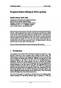
Fig. 7. Candidates generated by the rightmost expansion method when the label alphabet is {A,B}.

– Support Counting: Given the set of potentially frequent candidates, this phase consist of determining their actual support in D and keeping only those candidates that are actually frequent (a subset of the candidates generated in the previous phase). Other algorithms follow the FP-Growth [14] pattern growth approach and they do not explicitly generate candidates. For instance, the PathJoin algorithm [35] uses compacted structures called FPTrees to encode input data, while Chopper and XSpanner [34] use a sequential codification for trees and they extract frequent subtrees by discovering frequent subsequences. Since most algorithms follow the Apriori approach, we will first review several strategies that have been proposed for candidate subtree generation and support counting. Later, we delve into the implementation details of particular tree mining algorithms. 3.2. Candidate generation The first step in all Apriori-based pattern mining algorithms consists of generating a set of potentially frequent patterns. This set of candidate patterns is complete if it is a superset of the actual frequent pattern set. Several candidate generation strategies have been proposed for trees and all of the strategies we discuss in this paper are complete. They are also valid for all kinds of trees since they rely on the canonical tree representation schemes discussed in Section 2.2. We describe some candidate generation strategies in the following paragraphs: – Rightmost expansion The rightmost expansion strategy generates subtrees of size k+ 1 from frequent subtrees of size k by adding nodes only to the rightmost branch of the tree. Figure 7 illustrates candidate generation using rightmost expansion. It should be noted that, even though this candidate generation technique generates all potentially frequent patterns, it can also generate some duplicate patterns. For example, patterns t3 and t4 in Fig. 7 correspond to the same tree. Likewise, t1 and t2 also represent the same pattern.

A. Jim´enez et al. / Frequent itemset mining: A survey

611

Fig. 8. Two examples of trees with (left) and without (right) a prefix node.

The rightmost expansion candidate generation technique was used by some of the earlier tree mining algorithms, such as FreqT [1]. A specialization of this technique for candidate generation, which avoids the generation of duplicate candidates, is known as Tree-Model-Guided (TMG) candidate enumeration [13,26–28]. The TMG enumeration method uses embedded lists to represent the database trees. These lists contain, for each node of the tree, its descendants in a preorder enumeration. TMG enumeration uses references to the embedded lists of the trees in which a pattern appears, called occurrence coordinates, in order to represent each occurrence of the pattern in a tree. TGM uses the embedded lists and the occurrence coordinates to extend a candidate subtree by adding one node at the time starting from the last node of its rightmost path up to its root [27]. Another variant of the rightmost expansion technique using depth-sequence-based codification scheme was proposed in [4]. – Rightmost expansion with depth sequences This method was designed to identify patterns in unordered trees. It generates candidates that are always in canonical form to avoid the generation of duplicate candidates. As we explained in the previous section, when we use a depth sequence-based-codification a tree is represented with a sequence of pairs. When a new pair (d, l) is appended to the end of a canonical depth sequence, we are in fact connecting a new node to the rightmost path of the tree. It can be shown that the prefix of a canonical depth sequence is also a canonical depth sequence [4]. Therefore, if we only allow extensions to the canonical depth sequences representing frequent patterns that also lead to canonical depth sequences, we can avoid the generation of duplicate candidates. The depth sequence of a tree node is defined as the segment of the canonical sequence that matches with the bottom-up subtree rooted at the node. We say that a node is a prefix node when it is in the rightmost path of the tree and its depth sequence is a prefix of his left sibling’s depth sequence. The prefix node in the lowest level of the tree is called the lowest prefix node (not all trees have a lowest prefix node). When the tree has a lowest prefix node, the next prefix node is the descendant of the lowest prefix node’s left sibling that appears in the (i + 1)-th position of the left sibling’s depth sequence, being i the length of the depth sequence of the lowest prefix node. As shown in [8] based on the demonstration by [4], a pair (d, l) can be concatenated to the end of a canonical depth sequence S if and only if: ∗ d 6 d′ or (d=d′ and l > l′ ) where (d′ , l′ ) corresponds to the next prefix node when the tree has a lowest prefix node, and ∗ l > l′ if the rightmost path has a node at depth d with label l′ .

612

A. Jim´enez et al. / Frequent itemset mining: A survey

Fig. 9. Valid and invalid equivalence class-based extensions.

Figure 8 (a) shows a tree with two prefix nodes. The node number 9 is a prefix node because the bottom-up subtree rooted at this node has the codification (2,A), which is a prefix of its left sibling’s codification (node 7), i.e., (2,A) (3,B). The second prefix node in this tree is node 6, whose bottom-up subtree is (1,B) (2,A) (3,B) (2,A), which is a prefix of the bottom-up subtree rooted at its left sibling (node 1): (1,B) (2,A) (3,B) (2,A) (2,A). Node 6 is the lowest prefix node because it is at a lower level than node 9 in the tree, while node 5 is the next prefix node. Unlike the tree in Fig. 8 (a), the tree shown in Fig. 8 (b) does not have a lowest prefix node. The rightmost expansion candidate generation technique based on depth sequences has been used by Unot [4], uFreqt [21], Gaston [22], and TRIPS [29]. – Equivalence class-based extension The equivalence class-based extension technique is based on the depth-first canonical representation of trees and it was proposed by Zaki in [40]. Two trees of size k are in the same equivalence class if they share a (k − 1)-prefix in their depth-first canonical codification. Zaki’s candidate generation strategy generates a candidate (k + 1)-subtree by joining two frequent k-subtrees with (k − 1) nodes in common provided that they are in the same equivalence class. Let us consider the equivalence class whose prefix is ABA ↑↑ C. Figure 9 shows which extensions lead to elements belonging to this class and which ones do not. Adding a child node to node 0 (ABA ↑↑ C ↑ X) or node 3 (ABA ↑↑ C X) will lead to trees that belong to this equivalence class, while adding a child to node 1 (ABA ↑ X ↑↑ C) or node 2 (ABA X ↑↑↑ C) would lead to trees that do not belong to this class because they would not share the class prefix. This method avoids the generation of duplicates candidates. Zaki used this candidate generation technique in his TreeMiner [38] and SLEUTH [37] algorithms. Its derivatives, such as POTMiner [16], RETRO [7], or Phylominer [41], also employ this class-based extension method. – Right-and-left tree join The right-and-left tree join method was proposed in conjunction with the AMIOT algorithm [15]. In its candidate generation phase, this algorithm takes the rightmost and leftmost leaves of two trees of size k sharing the rest of their nodes in order to generate a candidate of size k + 1. Even though the naive implementation of this candidate generation strategy might easily lead to duplicate patterns, AMIOT interleaves its operations so that no duplicates are generated. Figure 10 shows the right-and-left tree join of a left tree L and a right tree R that only differ in one node: the leftmost leaf in L and the rightmost leaf in R. This join operation leads to a new tree that has the all nodes L and R share plus the two leaves that they do not have in common.

A. Jim´enez et al. / Frequent itemset mining: A survey

613

Fig. 10. Right and left tree join.

Fig. 11. Extension and join candidate generation [11]: Union of two sibling trees (top) and extension of the ABE ↑↑ C tree with a new node F (bottom).

– Extension and join The extension and join technique is based on the breadth-first codification of trees and it defines two operations to generate candidates: an extension mechanism to increase the tree depth and a join operation that expands the tree ‘width’ by joining two trees of size k that share k − 1 nodes to generate a new candidate of size k + 1. Figure 11 shows an example of the two operations required by the extension and join candidate generation procedure. It should be noted that the extension mechanism is needed because the join operation always produces trees that have the same height as their parents. This candidate generation method is used by HybridTreeMiner [11]. 3.3. Support counting Once we have generated the candidates it is necessary to check if they are actually frequent. Testing whether a given pattern is a subtree of a tree in the database is one of the most time-consuming operations in tree pattern mining algorithms. Therefore, it comes as no surprise that several techniques have been devised to make this test as efficient as possible. Many of the different proposals that can be found in the literature just use occurrence lists to represent the trees, following the approach already proposed by AprioriTID in 1994 [3]. These ancillary lists represent all the occurrences of each pattern X in the database (i.e. the tree database in vertical format) and they are designed so that you it is not necessary to perform tests on trees once these lists have been built. This occurrences are usually represented by the mapping between the pattern and the tree, i.e., the positions of the nodes in the database tree that match those of the pattern.

614

A. Jim´enez et al. / Frequent itemset mining: A survey

Fig. 12. Two trees (t1 and t2) and a pattern that is embedded in both trees.

Figure 12 shows two trees and a pattern that is a embedded subtree of both trees. The mappings of the pattern to the trees t1 and t2 are (0,2,5) and (0,1,3), respectively. Some of the different kinds of occurrence lists that have been proposed in the literature are the following: – Standard occurrence lists [11] preserve the identifiers of the trees as well as the matching between the pattern nodes and the database tree nodes using a breadth-first codification scheme. Each element of the occurrence list for pattern X has the form (tid, i1 . . . ik ), where tid is the tree identifier and i1 . . . ik represent the mapping between the nodes in the pattern X and those in the database tree. – Rightmost occurrence lists [1] only need to store the rightmost occurrence of X in each database tree, since rightmost expansion techniques do not have to take into account other occurrences of the pattern in the tree database (let us remember that these candidate generation strategies only had to append new nodes to the rightmost branch of a tree). Rightmost occurrence lists, also known as RMO-lists, are stored with each candidate and contain (tid, n) pairs, where n is the position of each tree node in the database tree tid that matches with the rightmost leaf of the candidate pattern. These lists are only useful for mining induced subtrees since they only preserve one node for each occurrence representing the whole subtree. Update operations can be performed on these lists as in AprioriTID [3] so that the RMO-list of a new k-pattern can be obtained from the RMO-lists of the k − 1 patterns it is generated from. – Scope-lists [38]: The previous occurrence lists can be used regardless of the candidate generation method used. However, scope-list are typically used with the equivalence class-based candidate generation technique because they are specially designed for it. These lists are composed of triplets (tid, m, s), where tid is the tree identifier, m is the mapping of the k − 1 prefix of the pattern X to the database tree, and s is the scope of the last node in X . The scope of a node n delimits the subtree rooted at n. Formally, the scope of a node is a pair [a, b] where a is the position of the node in the depth-first enumeration of the tree and b is the depth-first position of its rightmost descendant. – Vertical occurrence lists [13,28] group the occurrence coordinates of each subtree, as employed by the Tree Model Guide candidate generation method [27], which is a specialization of the rightmost extension technique we described in Section 3.2. Occurrence lists are usually sufficient for the efficient implementation of the support counting phase of Apriori-based tree pattern mining algorithms. However, other algorithms have resorted to more complex data structures. uFreqt [21] uses bipartite graphs to deal with the isomorphisms that might appear when working with unordered trees. Algorithms that follow the FP-Growth approach and those algorithms that have been devised for mining closed and maximal tree patterns also use special data structures, such as the FST-Forest structures employed by PathJoin [35]. This section has surveyed the main strategies used by the existing tree pattern mining algorithms. Tree pattern mining algorithms usually derive from Apriori [3] or FP-Growth [14]. Apriori-based algorithms

615

A. Jim´enez et al. / Frequent itemset mining: A survey Table 1 Frequent tree mining algorithms Algorithm FreqT [1] AMIOT [15] uFreqT [21] HybridTreeMiner [11] Unot [4] FreeTreeMiner [10] FreeTreeMiner’ [25] GASTON [22] X3Miner [26] MB3Miner [27] IMB3Miner [28] TreeMiner [38] TreeMinerD [38] RETRO [7] Chopper [34] XSpanner [34] Uni3 [13] Phylominer [41] SLEUTH [37] POTMiner [16] TRIPS [29] TIDES [29] CMTreeMiner [9] PathJoin [35] DRYADE [31] TreeFinder [30]

Ordered trees • •

Input trees Partially Unordered -ordered trees

• • • • • • • • • • • • • •

• • • •

Free trees

• • • •

Induced subtrees • • • • • • • •

•

•

• • • • • • • • • •

• • • • •

Identified patterns Embedded Incorporated subtrees /Subsumed

• • • • • • • • • • • • • •

Maximal /Closed

•

• •

• • • •

proceed in two phases: candidate generation and support counting. Several strategies have been proposed for the candidate generation phase: the rightmost extension strategy ensures that all the candidates are generated but it can also generate some duplicates, while the equivalence class-based extension, the right-and-left tree join, and the extension and join methods avoid the generation of duplicate patterns. Occurrence lists are often employed during the support counting phase to improve the performance of tree pattern mining algorithms. In particular, rightmost occurrence lists can be used for counting the occurrences of induced tree patterns, while scope-lists are usually employed in conjunction with the equivalence class-based candidate generation method to count the support of both induced and embedded tree patterns. 4. Tree mining algorithms In the previous section, we have described the main techniques behind most tree pattern mining algorithms. We now proceed to survey some of the particular frequent tree mining algorithms that have been proposed in the literature. Table 1 provides a bird’s-eye view of frequent tree mining algorithms. This table classifies pattern mining algorithms according to the kinds of input trees they can be applied to (ordered, partially-ordered, unordered, or free) and the kinds of subtrees they are able to identify within their input trees (induced, embedded, incorporated, or subsumed). This table also points out which of those algorithms have been specially devised for discovering closed and/or maximal tree patterns.

616

A. Jim´enez et al. / Frequent itemset mining: A survey

In the following paragraphs we will provide a brief overview of the algorithms collected in Table 1. For that, we will group these algorithms with respect to the kind of patterns they identify. 4.1. Identifying bottom-up subtrees There are not many tree mining algorithms specially designed to identify bottom-up subtrees because they can be represented as strings and sequence indexation techniques can be applied to mine them [24, 33]. Luccio et al. [19], for instance, create a sorted array with the canonical representation of each database tree and use binary search to determine if a pattern is a bottom-up subtree of the tree. 4.2. Identifying induced subtrees In this section, we focus our attention on the algorithms that identify induced subtrees and classify them according to the kinds of trees they can work with. 4.2.1. Induced subtrees in ordered trees FreqT [1] uses the rightmost expansion strategy to generate candidate trees. In the support counting phase, it resorts to rightmost occurrence lists (RMO-lists). AMIOT [15], which stands for Apriori-based Mining of Induced Ordered Trees, is based on the rightand-left tree join candidate generation strategy. As in FreqT, the support counting phase is performed with the help of RMO-lists. AMIOT uses ancillary lists (JL and JR lists) for each candidate to avoid the generation of duplicate candidates. This strategy has been shown to be more efficient than the rightmost expansion used by FreqT. 4.2.2. Induced subtrees in unordered trees The uFreqT [21] algorithm uses depth sequences to represent unordered trees in canonical form and it performs rightmost expansions to generate candidates. During the support counting phase for unordered trees, the main problem is to determine all the possible combinations of the children of a node v in the pattern that can match with the children of a node w in a database tree. These potential mappings can be efficiently represented by a bipartite graph G(v, w), for which a bipartite matching can be computed that maps each child of v to a different child of w. uFreqT uses an ancillary data structure that stores exactly those mappings that are included in some solvable bipartite graph G(v, w) for each node v in the rightmost path along with pointers to the database tree nodes in order to facilitate the support counting phase for unordered patterns. HybridTreeMiner [11] uses the breadth-first canonical codification of trees and the extension and join method for candidate generation. Occurrence lists are used for speeding up the support counting phase and the experiments performed show that HybridTreeMiner is faster than uFreqT. The Unot [4] algorithm uses depth sequences to canonically represent unordered trees. Rightmost expansion with depth sequences is used to generate frequent candidates. In order to speed up the support counting phase, Unot uses occurrence lists that are similar to HybridTreeMiner’s occurrence lists [11]. 4.2.3. Induced subtrees in free trees HybridTreeMiner can also be adapted to work with free trees by using a canonical representation of such trees and modifying the standard extension-and-join candidate generation method. HybridTreeMiner’s join procedure does not need to be modified for free trees. However, as we explained in section 2.2.4, free trees can be centered or bicentered. The extension mechanism must be

A. Jim´enez et al. / Frequent itemset mining: A survey

617

applied only to centered trees in order to generate all the needed candidate patterns, since bicentered trees do not have to be extended. FreeTreeMiner [10] is an earlier Apriori-based frequent pattern mining algorithm for free trees. Candidates of size k+1 are generated by combining pairs of frequent trees of size k sharing k−1 vertices, using the standard Apriori algorithm. Indexing techniques based on B+ trees and hash tables are used to speed up the support counting phase on trees. Experiments in [11] also show that HybridTreeMiner is more efficient than FreeTreeMiner. Another algorithm, which was also called FreeTreeMiner, was proposed in [25] and is shown as FreeTreeMiner’ in Table 1. This algorithm generates potentially frequent candidates by extending the leaves with maximum height in the tree (which are called extension points) and checks the support of each candidate by scanning the database (and saving the potential extensions in an extension table). While HybridTreeMiner is a descendant of Apriori, this algorithm is closer to gSpan [36], a graph mining algorithm. Finally, an algorithm to extracts induced pattern in free trees using paths of maximal length is proposed in the same paper that introduces GASTON [22], an efficient graph mining algorithm. 4.3. Identifying embedded subtrees Once we have described the algorithms that identify induced subtrees, we introduce those algorithms that help us to identify embedded subtrees. 4.3.1. Embedded subtrees in ordered trees Zaki’s TreeMiner [38] uses the depth-first codification of trees together with the class-based extension method to generate candidates. Zaki describes how you can prune the candidate generation phase in order to avoid the generation of duplicate candidates using his method, as we discussed in section 3.2. Scope-lists are used by TreeMiner to determine the support of each pattern. These scope-lists can be built by joining the scope-lists of the subtrees involved in the candidate generation, thus eliminating the need to access to the tree database once the initial scope-list have been built. TreeMinerD [38] is a variant of TreeMiner that is more efficient than TreeMiner in case we are interested in obtaining the patterns support instead of their weighted support (see Section 2). Chopper [34] is an FP-Growth-based algorithm to identify embedded subtrees in ordered trees that employs a depth-sequence-based codification. This algorithm has two main phases: first, it applies an algorithm to mine frequent sequences and then, using these sequences, it determines which sequences correspond to frequents subtrees in the original database. XSpanner [34] is a variant of Chopper that integrates Chopper’s two phases in order to improve its efficiency. Chopper and XSpanner are reported to be more efficient than TreeMiner. XSpanner and Chopper can save time and space cost by avoiding false candidate generation, while the performance of XSpanner is more stable than that of Chopper [34]. Finally, X3Miner [26], MB3-Miner [27] and IMB3-Miner [28] are algorithms that generate candidates by using the Tree Model Guided (TMG) enumeration, a specialization of the rightmost path extension method that avoids the generation of duplicate candidates. Vertical occurrence lists are used to aid in the support counting phase. MB3 variants ensure that only valid candidates are generated, while the join approach used in TreeMiner can generate many false subtrees, which degrades its performance [28].

618

A. Jim´enez et al. / Frequent itemset mining: A survey

4.3.2. Embedded subtrees in unordered trees SLEUTH [37] is Zaki’s proposal for mining unordered trees. As in TreeMiner, Zaki resorts to the depth-first canonical codification for representing unordered trees and scope-lists for the support counting phase. In order to generate all the candidates, however, it is sometimes necessary to use non-canonical trees to build a canonical one. Hence, Zaki proposes two alternative techniques to generate candidates: – Using the class-based extension mechanism, but checking if each subtree is canonical before extending it with the elements of its equivalence class. – Using the canonical extension which extends trees with the elements that belong to the same class and also with those belonging to the subtree classes of size 2 that share the node that is going to be extended, but only if the result is in canonical form. Canonical extension generates non-redundant candidates, but many of them may not be frequent. On the other hand, class-based extension generates redundant candidates, but considers a smaller number of potential frequent candidate extensions. The experiments in [37] demonstrate that the class-based extension method is more efficient that the canonical extension. Phylominer [41] is a special-purpose algorithm devised to identify embedded subtrees in Phylogenetic trees, which can be defined as rooted leaf-labeled unordered trees where all internal nodes have no labels, being the fan-out of each internal node (i.e. its number of children) at least 2. The Uni3 [13] algorithm is yet another variant of IMB3Miner [28] to identify patterns in unordered trees using the TMG candidate generation technique. 4.3.3. Embedded subtrees in both ordered and unordered trees TRIPS and TIDES [29] are two algorithms designed to identify embedded subtrees in ordered or unordered trees. They use embedded lists to generate candidates and an ancillary hash table, dubbed support structure, to aid in the support counting phase. The difference between these two algorithms is their canonical representation: TRIPS uses a post-order traversal representation (numbered Pr¨ufer sequences [12]) while TIDES employs depth sequences. POTMiner [16] is a variant of the TreeMiner/SLEUTH tandem that can be used to mine induced and embedded subtrees in ordered, unordered, and partially-ordered trees. As its predecessors, POTMiner uses Zaki’s class-based extension method to generate candidates and scope-lists during the support counting phase. 4.4. Identifying incorporated and subsumed subtrees RETRO [7] is yet another variant of TreeMiner. In this case, this algorithm can be used to identify incorporated and subsumed subtrees, as well as the more usual induced and embedded tree patterns. The TreeFinder algorithm [30] uses the Apriori-based candidate generation technique based on ancestor-descendent relationships in order to discover subsumed subtrees. We will return to this algorithm in the following section. 4.5. Closed and maximal subtrees This final section deals with those algorithms that identify closed and maximal subtrees. Again, we can further classify them depending on the kind of subtrees they identify (induced or embedded).

A. Jim´enez et al. / Frequent itemset mining: A survey

619

4.5.1. Closed and maximal induced subtrees In CMTreeMiner [9], an enumeration DAG (directed acyclic graph) is a lattice-like data structure that represents all frequent subtrees. Enumeration trees, which are sometimes used for frequent itemset mining, are just spanning trees of these enumeration DAGs. An enumeration DAG joins each frequent k-subtree t with the (k − 1)-subtrees that can be extended to obtain t, as well as with the (k + 1)-subtrees that can be obtained by extending t. This DAG can then be used to prune the set of frequent patterns and generate only those patterns that are maximal. Pruning techniques have been devised in CMTreeMiner for improving the efficiency of closed and maximal subtree mining in ordered and unordered trees. PathJoin [35] discovers maximal frequent induced subtrees from a database of unordered labeled trees. It employs a specialized data structure, a Frequent-Subtree Forest or FST-Forest, that is used to represent frequent trees in a compact form and improve the efficiency of the support counting phase. 4.5.2. Closed and maximal embedded subtrees As mentioned above, the TreeFinder algorithm [30] uses the plain Apriori-based candidate generation technique, albeit it applies this technique directly to ancestor-descendent relationships instead of the other candidate generation strategies we have discussed in this paper. This direct use of ancestor-descendent relationships lets TreeFinder discover subsumed subtrees (see Section 2). Once frequent relationships are clustered by their support count, it is very easy to determine whether a particular candidate is frequent. However, it should be noted that this method is not complete: TreeFinder is an approximate miner. In the general case, it is only guaranteed to find a subset of the actual frequent trees. DRYADE [31], on its hand, searches for closed patterns in tree databases (recall that closed patterns are not necessarily maximal). Discovering the closed frequent patterns of depth 1 is the basic mechanism behind DRYADE. Then, they are hooked together in order to build higher-depth closed frequent patterns in a level-wise fashion. DRYADE reformulates search operations in a propositional language. This way, DRYADE can benefit from any progress made in the field of closed itemset mining algorithms, since it just delegates on a standard closed itemset mining algorithm. DryadeParent is a variant of the original DRYADE algorithm that outperforms CMTreeMiner by several orders of magnitude on datasets where the frequent patterns have a high branching factor [32]. In this section, we have reviewed the better-known tree mining algorithms that have been proposed in the literature. We have classified them according to the kind of patterns they can identify and also according to the kind of trees they can deal with (see Table 1). AMIOT [15] has been shown to be more efficient than FREQT [1] for induced subtrees in ordered trees, while HybridTreeMiner [11] and Unot [4] obtain better results for unordered trees. HybridTreeMiner [11] can also used for mining free trees, as well as both FreeTreeMiners [10,25] and GASTON [22]. Finally, TreeMiner [38] and SLEUTH [37] are two well-known Apriori-based algorithms for mining embedded subtrees, whereas Chopper and XSpanner [34] are FP-Growth based algorithms that have been reported to be more efficient for ordered trees.

5. Conclusions In this paper, we have studied existing tree mining algorithms. First, we introduced some basic terminology and definitions. Later, we discussed the usual strategies frequent tree mining algorithms

620

A. Jim´enez et al. / Frequent itemset mining: A survey Table 2 Main features of the different frequent tree mining algorithms analyzed in this survey

Algorithm FreqT [1] AMIOT [15] uFreqT [21]

Tree representation − − Depth sequences

HybridTreeMiner [11] FreeTreeMiner [10] FreeTreeMiner’ [25] TreeMiner [38] TreeMinerD [38]

Breadth-first codification Depth-first codification Depth-first codification Depth-first codification Depth-first codification

Candidate generation approach Rightmost expansion Right and left union Rightmost expansion with depth sequences Union-extension method Apriori itemset generation Maximal-depth extension Equivalence classes Equivalence classes

RETRO [7] Chopper [34]

Relational representation Depth sequences

Equivalence classes N/A

X3Miner [26]

Depth-first codification

MB3Miner [27]

Depth-first codification

IMB3Miner [28]

Depth-first codification

XSpanner [34]

Depth sequences

Rightmost expansion – TMG enumeration Rightmost expansion – TMG enumeration Rightmost expansion – TMG enumeration N/A

SLEUTH [37] Unot [4]

Depth-first codification Depth sequences

Phylominer [41] Uni3 [13]

Depth-first codification Depth-first codification

GASTON [22]

Depth sequences

TRIPS [29] TIDES [29]

Post-order codification Depth sequences

POTMiner [16] CMTreeMiner [9] TreeFinder [30] PathJoin [35] DRYADE [31]

Depth-first codification Depth-first codification Relational representation FST-Forest structure Propositional language

Equivalence classes Rightmost expansion with depth sequences Equivalence classes Rightmost expansion – TMG enumeration Rightmost expansion with depth sequences Embedding lists Rightmost expansion with depth sequences Equivalence classes N/A Apriori itemset generation N/A −

Implementation details RMO occurrence lists RMO occurrence lists Bipartite graphs Occurrence lists Indexation techniques Scope lists Scope lists for non-weighted support Scope lists Frequent subsequences (PrefixSpan [23]) Vertical occurrence lists Vertical occurrence lists Vertical occurrence lists Frequent subsequences (PrefixSpan [23]) Scope lists Occurrence lists No labels in internal nodes Vertical occurrence lists

Support Structure (hash table) Support Structure (hash table) Scope lists DAG enumeration graph Clustering techniques External closed itemset miner

employ in order to create a consistent framework that lets us easily understand the details behind the implementation of particular frequent tree mining algorithms. We have classified existing algorithms according to the kind of trees each algorithm is designed to work with (ordered, unordered, partially-ordered, and free trees) as well as the kind of patterns they are able to identify (induced, embedded, incorporated, subsumed, closed, and maximal). Table 2 summarizes the main features of the tree mining algorithms described in this paper: their underlying tree representation mechanism, their candidate generation strategy (where applicable), and some relevant implementation details that are needed for their efficient implementation. Table 2 shows that most tree mining algorithms follow the well-known Apriori approach [3], while only a few employ the FP-Growth [14] pattern growth strategy. Within the Apriori-based algorithms we have surveyed, most of them resort to the right-most expansion method or employ Zaki’s class-based extension technique for candidate generation. Vertical, RMO, or plain occurrence lists are typically used with the former, while scope-lists are used with the latter in order to speed up the support counting phase.

A. Jim´enez et al. / Frequent itemset mining: A survey

621

Acknowledgements Work partially supported by research projects TIN2006-07262 (Spanish Ministry of Science and Innovation), TIN2009-08296 (Spanish Ministry of Science and Innovation) and P07-TIC-03175 (Junta de Andaluc´ıa). References [1] [2] [3] [4] [5] [6] [7] [8] [9] [10] [11] [12] [13] [14] [15] [16] [17] [18] [19] [20] [21] [22]

A. Kenji, K. Shinji, A. Tatsuya, A. Hiroki and A. Setsuo, Efficient substructure discovery from large semi-structured data. In Proceedings of the 2nd SIAM International Conference on Data Mining, 2002. C. Charu, Aggarwal, Na Ta, J.Y. Wang, J.H. Feng and M.J. Zaki, Xproj: a framework for projected structural clustering of XML documents. In Proceedings of the 13th ACM SIGKDD International Conference on Knowledge Discovery and Data Mining, August 12–15, 2007, pp. 46–55. R. Agrawal and R. Srikant, Fast algorithms for mining association rules in large databases. In Proceedings of 20th International Conference on Very Large Data Bases, September 12–15, 1994, pp. 487–499. T. Asai, H. Arimura, T. Uno and S. ichi Nakano, Discovering frequent substructures in large unordered trees. In Discovery Science, volume 2843 of Lecture Notes in Artificial Intelligence, Springer, 2003, pp. 47–61. C. Borgelt and M.R. Berthold, Mining molecular fragments: Finding relevant substructures of molecules. In Proceedings of the 2nd IEEE International Conference on Data Mining, 2002, pp. 51–59. B. Bringmann, Matching in frequent tree discovery. In Proceedings of the 4th IEEE International Conference on Data Mining, 1-4 November, Brighton, UK, 2004, pp. 335–338. B. Bringmann, To see the wood for the trees: Mining frequent tree patterns. In Constraint-Based Mining and Inductive Databases, European Workshop on Inductive Databases and Constraint Based Mining, Hinterzarten, Germany, March 11–13, 2004, Revised Selected Papers, volume 3848 of Lecture Notes in Computer Science, Springer, 2006, pp. 38–63. Y. Chi, R.R. Muntz, S. Nijssen and J.N. Kok, Frequent subtree mining – an overview, Fundamenta Informaticae 66(1–2) (2005), 161–198. Y. Chi, Y. Xia, Y. Yang and R.R. Muntz, Mining closed and maximal frequent subtrees from databases of labeled rooted trees, IEEE Transactions on Knowledge and Data Engineering 17(2) (2005), 190–202. Y. Chi, Y. Yang and R.R. Muntz, Indexing and mining free trees. In Proceedings of the 3rd IEEE International Conference on Data Mining, 2003, pp. 509–512. Y. Chi, Y. Yang and R.R. Muntz, HybridTreeMiner: An efficient algorithm for mining frequent rooted trees and free trees using canonical form. In The 16th International Conference on Scientific and Statistical Database Management, 2004, pp. 11–20. J. Dieter, In Graphs, Networks and Algorithms, volume 5 of Algorithms and Computation in Mathematics. Springer, 2007. F. Hadzic, H. Tan and T.S. Dillon, Uni3 – efficient algorithm for mining unordered induced subtrees using tmg candidate generation. In Computational Intelligence and Data Mining, 2007, pp. 568–575. J. Han, J. Pei and Y. Yin, Mining frequent patterns without candidate generation. In Proceedings of the 6th ACM SIGKDD Interna-tional Conference on Knowledge Discovery and Data Mining, 2000, pp. 1–12. S. Hido and H. Kawano, AMIOT: induced ordered tree mining in tree-structured databases. In Proceedings of the 5th IEEE International Conference on Data Mining, 2005, pp. 170–177. A. Jimenez, F. Berzal and J. Carlos Cubero, Mining induced and embedded subtrees in ordered, unordered, and partiallyordered trees. In the 17th International Symposium on Methodologies for Intelligent Systems, volume 4994 of Lecture Notes in Artificial Intelligence, Springer, 2008, pp. 111–120. J.M. Kleinberg, Challenges in mining social network data: processes, privacy, and paradoxes. In Proceedings of the 13th ACM SIGKDD International Conference on Knowledge Discovery and Data Mining, San Jose, California, USA, August 12–15, 2007, 2007, pp. 4–5. R. Kosala and H. Blockeel, Web mining research: A survey, SIGKDD Explorations 2(1) (2000), 1–15. F. Luccio, A. Mesa Enriquez, P. Olivares Rieumont and L. Pagli, Exact rooted subtree matching in sublinear time. In ANaCC/ACM/IEEE Inter- national Congress on Computer Science, CENIDET, 2002, pp. 27–35. R. Nayak and M. Javeed Zaki, eds, Proceedings of the First International Workshop of Knowledge Discovery from XML Docu- ments,Singapore, April 9, volume 3915 of Lecture Notes in Computer Science. Springer, 2006. S. Nijssen and J.N. Kok. Efficient discovery of frequent unordered trees. In First International Workshop on Mining Graphs, Trees and Sequences (MGTS2003), in conjunction with ECML/PKDD’03, 2003, pp. 55–64. S. Nijssen and J.N. Kok, A quickstart in frequent structure mining can make a difference. In Proceedings of the 10th ACM SIGKDD International Conference on Knowledge Discovery and Data Mining, 2004, pp. 647–652.

622 [23] [24] [25] [26] [27] [28] [29] [30] [31] [32] [33] [34] [35] [36] [37] [38] [39] [40] [41]

A. Jim´enez et al. / Frequent itemset mining: A survey Jian Pei, Jiawei Han, Bezhad Mortazavi-Asl, Helen Pinto, Qiming Chen, Umeshwar Dayal, and Mei-Chun Hsu. Prefixspan: Mining sequential patterns efficiently by prefix-projected pattern growth. In Proceedings of the 17th International Conference on Data Engineering, 2001, pp. 215–225. B. Phoophakdee and M.J. Zaki, Genome-scale disk-based suffix tree indexing. In Proceedings of the 27th ACM SIGMOD International Conference on Management of Data, 2007, pp. 833–844. U. R¨uckert and S. Kramer, Frequent free tree discovery in graph data. In Proceedings of the 2004 ACM symposium on Applied computing, 2004, pp. 564–570. H. Tan, T.S. Dillon, L. Feng, E. Chang and F. Hadzic, X3-Miner: Mining Patterns from an XML Database. In The 6th International Conference on Data Mining, Text Mining and their Business Applications, May 2005, Skiathos, Greece, 2005, pp. 287–296. H. Tan, T.S. Dillon, F. Hadzic, E. Chang and L. Feng, MB3-Miner: mining eMBedded subTREEs using Tree Model Guided candidate generation. In Proceedings of the First International Workshop on Mining Complex Data, 2005, pp. 103–110. H. Tan, T.S. Dillon, F. Hadzic, E. Chang and L. Feng, IMB3-Miner: Mining induced/embedded subtrees by constraining the level of embedding. In Proceedings of the 10th Pacific-Asia Conference on Knowledge Discovery and Data Mining, 2006, pp. 450–461. Shirish Tatikonda, Srinivasan Parthasarathy, and Tahsin Kurc. TRIPS and TIDES: new algorithms for tree mining. In Proceedings of the 15th ACM International Conference on Information and Knowledge Management, 2006, pp. 455–464. A. Termier, M.-C. Rousset and M. Sebag, TreeFinder: a first step towards XML data mining. In Proceedings of the 2nd IEEE International Conference on Data Mining, 2002, pp. 450–457. Alexandre Termier, Marie-Christine Rousset, and Michele Sebag. DRYADE: a new approach for discovering closed frequent trees in heterogeneous tree databases. In Proceedings of the 4th IEEE International Conference on Data Mining, 2004, pp. 543–546. A. Termier, M.-C. Rousset, M. Sebag, K. Ohara, T. Washio and H. Motoda, Efficient mining of high branching factor attribute trees. In Proceedings of the 5th IEEE International Conference on Data Mining, 2005, pp. 785–788. Y. Tian, S. Tata, R.A. Hankins and J.M. Patel, Practical methods for constructing suffix trees. In Proceedings of the 31st International Conference on Very Large Data Bases, volume 14, 2005, pp. 281–299. C. Wang, M. Hong, J. Pei, H. Zhou, W. Wang and B. Shi, Efficient patterngrowth methods for frequent tree pattern mining. In Proceedings of the 8th Pacific-Asia Conference on Knowledge Discovery and Data Mining, volume 3056 of Lecture Notes in Computer Science, Springer, 2004, pp. 441–451. Y. Xiao, J.-F. Yao, Z. Li and M.H. Dunham, Efficient data mining for maximal frequent subtrees. In Proceedings of the 3rd IEEE International Conference on Data Mining, 2003, pp. 379–386. X. Yan and J. Han, gSpan: Graph-based substructure pattern mining. In Proceedings of the 2nd IEEE International Conference on Data Mining, pp. 721–724, 2002. M.J. Zaki, Efficiently mining frequent embedded unordered trees, Fundamenta Informaticae 66(1–2) (2005), 33–52. M.J. Zaki, Efficiently mining frequent trees in a forest: Algorithms and applications, IEEE Transactions on Knowledge and Data Engineering 17(8) (2005), 1021–1035. M.J. Zaki and C.C. Aggarwal, XRules: an effective structural classifier for XML data. In Proceedings of the 9th ACM SIGKDD International Conference on Knowledge Discovery and Data Mining, (2003), pp. 316–325. M.J. Zaki, Efficiently mining frequent trees in a forest. In Proceedings of the 8th ACM SIGKDD International Conference on Knowledge Discovery and Data Mining, July 23–26, 2002, pp. 71–80. S. Zhang and J.T.L. Wang, Discovering frequent agreement subtrees from phylogenetic data, IEEE Transactions on Knowledge and Data Engineering 20(1) (2008), 68–82.