Fresh-Register Automata Nikos Tzevelekos Oxford University Computing Laboratory
[email protected]
Abstract
Our model is based on the successful paradigm of FiniteMemory Automata (FMA), introduced by Kaminski and Francez in the early 90’s [11]. Motivated by real-world problems (where codes, addresses, identifiers, etc. may have unbounded domains), those automata address a demand for a “natural” finite-state machine model over infinite alphabets. An FMA A is an automaton attached with a finite number of name-storing registers. Its structure looks identical to that of an ordinary finite-state automaton over a finite set of labels generated by indices in the range 1, . . . , n, where n is the number of registers. However, A truly operates on the infinite set of inputs A (the set of names), with indices i referring to the names stored in the i-th register of A. This simple idea lifts the automaton from finite to infinite alphabet. There are two ways in which an FMA can access its registers: either by comparing an input name to a stored one, or by storing an input name in one of its registers but only in case it is locally fresh, that is, it does not already appear in any of them. Thus, FMA’s are history-free: their computational steps rely solely on their current registers. Here we introduce Fresh-Register Automata (FRA), a finite-register automaton model which extends FMA’s by global freshness recognition: an automaton can now accept (and store) an input name just in case it is fresh in the whole run. For example, a transition
What is a basic automata-theoretic model of computation with names and fresh-name generation? We introduce Fresh-Register Automata (FRA), a new class of automata which operate on an infinite alphabet of names and use a finite number of registers to store fresh names, and to compare incoming names with previously stored ones. These finite machines extend Kaminski and Francez’s Finite-Memory Automata by being able to recognise globally fresh inputs, that is, names fresh in the whole current run. We examine the expressivity of FRA’s both from the aspect of accepted languages and of bisimulation equivalence. We establish primary properties and connections between automata of this kind, and answer key decidability questions. As a demonstrating example, we express the theory of the pi-calculus in FRA’s and characterise bisimulation equivalence by an appropriate, and decidable in the finitary case, notion in these automata. Categories and Subject Descriptors F.1.1 [Computation by Abstract Devices]: Models of Computation; D.3.1 [Programming Languages]: Formal Definitions and Theory—Semantics General Terms
Theory, Languages, Verification
1. Introduction
i⊛
q −→ q ′ means that if A is at state q and the set of names that have appeared in its registers so far is H, then A can accept any name a ∈ / H, store it in its i-th register and proceed to q ′ . This history-sensitive feature precisely captures fresh-name creation.1 Thus, e.g. the following language (not recognised by FMA’s [11]) is recognised by a singlestate FRA with one register.
One of the most common and useful abstractions in programming is the assumption that entities of specific kinds can be created at will and, moreover, in such a manner that newly created entities are always fresh — distinct from any other such created thus far. This is, for example, the case with mutable reference cells, exceptions user-declared datatypes, etc. in languages like Standard ML [15]. Following a long tradition in computer science [20], we call these entities names and specify them as follows.
L1 = { a1 · · · ak ∈ A∗ | ∀i 6= j. ai 6= aj } An intuitive way to view L1 is as the trace of a fresh-name generator: one which returns reference cells in SML, objects in Java, memory addresses in C, etc. Research in FMA’s and their formal languages has been extensive [2, 6, 11, 21, 25, 27]. It has been shown [11, 21] that FMA-recognisable languages are closed under union, intersection, concatenation and Kleene star; they are not closed under complement; emptiness of FMA’s is decidable; and universality is undecidable. Our first contribution is to answer this series of questions for FRA’s. We show that for emptiness and universality the situation remains the same as in FMA’s. On the other hand, FRArecognisable languages are still closed under union and intersection, but history-sensitiveness prohibits this for concatenation and Kleene star. Moreover, they are not closed under complement and, in fact, there is an FMA-recognisable language whose complement is not recognised by FRA’s.
Names can be created fresh dynamically and locally, compared for equality and communicated between agents or subroutines. Apart from the uses mentioned above, names form the basis of calculi of mobile processes (e.g. the π-calculus [14]); appear in network protocols and secure transactions; and are generally essential in programming for identifying variables, channels, threads, objects, codes, and many other sorts of name in disguise. To our knowledge, there has not been in the literature a proposal of a basic automata-theoretic model of names, providing abstract machines underlying all these paradigms. We propose just such a model here.
1 Note
that, although history-sensitive, the automaton does not have full access to the history H. In automata-theoretic jargon, the situation can be described as consulting an oracle who can decide the freshness of names.
Revised version 18/11/2010.
1
Our main vehicle for studying equivalence between FRA’s is bisimulation equivalence (also called bisimilarity). The notion is very relevant from the point of view of programming, and process calculi in particular, and in the case of FRA’s it implies language equivalence. More importantly, we show that by examining FRA’s at the symbolic level, i.e. as ordinary finite-state automata on the set of index-generated labels, it is possible to capture bisimilarity by an appropriate symbolic notion; we thus prove that FRAbisimilarity is decidable. A symbolic bisimulation relates states of two automata in specific environments, the latter specifying how are the names which appear in their registers related. As a demonstrating example, we express the π-calculus in the context of fresh-register automata. We introduce the xπ-calculus system: a presentation of the π-calculus with early transition semantics [14, 26], in which processes are states of an infinite FRA. Transitions are given by FRA-transitions and the system is finitely branching. More specifically, bound outputs are modelled by globally fresh transitions, while each input is decomposed into finitely many cases: either the incoming name is locally fresh or it already appears in the registers. This clean treatment of fresh and bound names is the main advantage of the xπ-calculus and allows for the finite representation, as ordinary FRA’s, of finitary processes.2 Moreover, we characterise strong bisimilarity by an appropriate symbolic notion in xπ. This gives an alternative proof of decidability of bisimilarity for finitary processes.
HD-transitions match ‘on-the-fly’ names between the source, target, and label of π-calculus transitions, allowing thus for the use of representatives of processes and transitions, rather than all possible ones under e.g. permutation of fresh names. The stream of research on HD-automata has focussed both on foundational issues [17, 22] and on pragmatic applications [7]. The work presented here shares objectives with HD-automata, and to some extent can be viewed as a complementary attempt to the same question, albeit based on basic machines of “first principles”.
Motivation and related work
Constants have an auxiliary role and are non-storable.3 We let a, b, etc. range over names. We write A∗ for the set of finite strings of names, and A⊛ for its restriction to those containing pairwise distinct names. Strings a1 · · · an will be typically represented by vectors ~a, in which case img(~a) = {a1 , . . . , an }. For each n ∈ ω, we write [n] for the set {1, . . . , n}, and let
Outline In the next section we give the basic definitions on FRA’s. Section 3 provides some useful bisimilar constructions. In Section 4 we recall FMA’s and establish their connection to FRA’s. We examine WFRA’s, a weaker notion of FRA’s focussing on global freshness, in Section 5. In Section 6 we prove some technical results regarding closure properties for FRA’s, and in Section 7 we show that emptiness and bisimilarity are decidable using symbolic methods. Section 8 examines the π-calculus in the setting of FRA’s.
2. Definitions We distinguish between two sets of input symbols: • an infinite set of names, A, and • a finite set of constants, C.
Programming languages The idea of studying names in higherorder languages and in isolation of other effects was first pursued by Pitts and Stark [24]. They introduced the ν-calculus, an extension of the simply-typed λ-calculus with references of unit type. Investigations on the ν-calculus were meticulously carried on by Stark in his PhD thesis [28], which exposed a rather unexpected complexity hidden behind names. It became evident that better models for languages with names were needed. To address this, new directions in denotational [1, 12, 13, 18] and operational [3, 10] models were explored, significantly advancing our understanding of computation with names but, at the same time, leaving basic questions unanswered. In particular, those works examined computation at the higher level, that of programs and program equivalence, leaving open the question of a basic, lower-level model. Interestingly, in their initial paper on FMA’s [11], Kaminski and Francez motivate their construction (also) by briefly presenting an idealised procedural language with names. There, names cannot be freshly created, but they can be read from the environment as inputs and stored in a finite memory. Moreover, stored names can flow inside the memory from one register to another and can also be compared for equality and thus trigger goto’s. The authors explain that FMA’s operate like acceptors for that simple imperative language with names. By analogy, FRA’s describe the extension of the language with fresh-name generation.
Ln = C ∪ { i, i• , i⊛ | i ∈ [n] } . be the set of labels generated by [n]. Moreover, we define Regn = { σ : [n] → A∪{♯} | ∀i 6= j. σ(i) = σ(j) =⇒ σ(i) = ♯ } to be the set of register assignments of size n. We write img(σ) for the name-range of σ, i.e. img(σ) = { a ∈ A | ∃i. σ(i) = a }, and let dom(σ) = { i ∈ [n] | σ(i) ∈ A }. Whenever a ∈ / img(σ), σ[i 7→ a] = { (i, a) } ∪ { (j, σ(j)) | j ∈ [n] \ {i} } is an update of σ, for any i ∈ [n]. Definition 1. A fresh-register automaton (FRA) of n registers is a quintuple A = hQ, q0 , σ0 , δ, F i where: • • • • •
Process calculi For mobile systems like the π-calculus [14], where processes can create locally, receive or send names, the use of ordinary labelled transition systems for its semantics is in many ways unsatisfactory: for example, infinite branching arises even in the case of very simple processes that receive a (locally fresh) name, or output a locally created (globally fresh) one. Such shortcomings naturally led to solutions involving representations of processes by formalisms which incorporate name-reasoning of some sort [4, 5, 16]. The most notable paradigm in this direction is that of History-Dependent Automata (HD-Automata) [16, 22], which are structures defined in a universe of named sets and named functions. HD-automata can succinctly represent the π-calculus, as 2A
Q is a finite set of states, q0 is the initial state, σ0 ∈ Regn is the initial register assignment, δ ⊆ Q × Ln × Q is the transition relation, F ⊆ Q is the set of final states.
A is called a register automaton (RA) if there are no q, q ′ , i such that (q, i⊛ , q ′ ) ∈ δ. Transitions containing labels of the form i are called known transitions; those of the form i• are locally fresh ones; and globally fresh transitions involve i⊛ . Thus, an RA is an FRA with no globally fresh transitions.4 Here is an informal reading of δ. Suppose A is at state q1 with current register assignment σ. If input ℓ ∈ C ∪ A arrives then:5 3 In
other presentations [11, 21] there is no such distinction, but symbols that appear in the initial register assignment can play the role of constants. 4 This yields the same notion of register automaton as that of [21]. 5 Note that the same symbol, ℓ, is later used to range over elements of L . n
process is finitary if its it does not grow unboundedly in parallelism.
2
• If ℓ ∈ C and (q1 , ℓ, q2 ) ∈ δ then A accepts ℓ and moves to q2 .
with initial assignment {(1, ♯)}. The automaton works as follows. It receives a name a and then keeps receiving a until some b 6= a arrives; then it keeps receiving b until a globally fresh c arrives; it then repeats from start. Thus, members of L(A) are of the form
• If ℓ ∈ A and (q1 , i, q2 ) ∈ δ and σ(i) = ℓ then A accepts ℓ and
moves to q2 . • If ℓ ∈ A and (q1 , i• , q2 ) ∈ δ and ℓ is not stored in σ then A
aj00 bk0 0 c0 aj11 bk1 1 c1 aj22 bk2 2 c2 . . . ajnn bknn cn
accepts ℓ, it sets σ(i) = ℓ and moves to q2 .
where, for all i, we have ji , ki > 0, ai 6= bi and ci differs from all symbols preceding it. Formally, setting
• If ℓ ∈ A and (q1 , i⊛ , q2 ) ∈ δ and ℓ ∈ / img(σ0 ) and ℓ has not
appeared in the current run then A accepts ℓ, it sets σ(i) = ℓ and moves to q2 .
L′ (H) = { an1 bn2 c | ni > 0 ∧ a 6= b ∧ c ∈ / H ∪ {a, b} } S we have that L(A) = i∈ω Li , where we set L0 = L′ (∅) and Li+1 = { ~a ~b | ~a ∈ Li ∧ ~b ∈ L′ (img(~a)) } .
The above is formally defined by means of configurations representing the intended current state of the automaton, which apart from states contains information on the current register assignment and the set of names having appeared thus far (the history). The latter component is necessary for globally fresh transitions. ˆ = Q × Regn × Pfn (A) Q
Some basic results The languages of FMA’s [11] are regular once constrained to a finite number of symbols. Moreover, the language accepted by an FMA is impervious to name-permutations that do not affect its initial register. These properties carry over to FRA’s, and are proved as in [11].
and Pfn (A) being the set of finite subsets of A. From δ define a transition relation on configurations
Proposition 5. Let A = hQ, q0 , σ0 , δ, F i be an FRA of n registers and S ⊆ A be finite. Then, L(A) ∩ S ∗ is a regular language.
ˆ with Definition 2. A configuration of A is a triple (q, σ, H) ∈ Q,
ˆ × (C ∪ A) × Q ˆ −→δ ⊆ Q
∼ =
Proposition 6. For A as above, if ~a ∈ L(A) and π : A → A is such that π(a) = a for all a ∈ img(σ0 ) then π(~a) ∈ L(A).
ˆ and (q, ℓ, q ′ ) ∈ δ: as follows. For all (q, σ, H) ∈ Q
Bisimulation Bisimulation equivalence turns out to be a great tool for relating automata, even from different paradigms. It implies language equivalence and, in all our cases of interest, it is not too strict in this aspect. We choose it here as our main vehicle of study.
ℓ
• If ℓ ∈ C then (q, σ, H) −→δ (q ′ , σ, H). a • If ℓ = i and σ(i) = a then (q, σ, H) −→δ (q ′ , σ, H ∪ {a}). a • If ℓ = i• and a ∈ / img(σ) then (q, σ, H) −→δ (q ′ , σ ′ , H ′ )
with σ ′ = σ[i 7→ a] and H ′ = H ∪ {a}. a • If ℓ = i⊛ and a ∈ / H∪img(σ0 ) then (q, σ, H) −→δ (q ′ , σ ′ , H ′ ) ′ ′ with σ = σ[i 7→ a] and H = H ∪ {a}.
Definition 7. Let Ai = hQi , q0i , σ0i , δi , Fi i be FRA’s with ni ˆ1 × Q ˆ 2 is called a registers, for i = 1, 2. A relation R ⊆ Q simulation on A1 and A2 if, for all (ˆ q1 , qˆ2 ) ∈ R,
We write −→ −→δ for the reflexive transitive closure of −→δ .
• if π1 (ˆ q1 ) ∈ F1 then π1 (ˆ q2 ) ∈ F2 , ~ ℓ
ℓ
R is called a bisimulation if both R and R−1 are simulations. We say that A1 and A2 are bisimilar, written A1 ∼ A2 , if there is a bisimulation R such that ((q01 , σ01 , ∅), (q02 , σ02 , ∅)) ∈ R.
~ ℓ L(A) = { ~ ℓ ∈ (A ∪ C)∗ | (q0 , σ0 , ∅) −→ −→δ (q, σ, H) ∧ q ∈ F }
Lemma 8. If A1 ∼ A2 then L(A1 ) = L(A2 ).
and is called the language recognised by A. Two automata are equivalent if they recognise the same language.
The above is proved using standard methods. Bisimilarity is also called bisimulation equivalence. For instance, the automaton A0 of example 4 is bisimilar to
Remark 3. There is an equivalent definition of FRA’s in which histories include img(σ0 ) by default, and in which reachable configurations are the ones reached from (q0 , σ0 , img(σ0 )). Here instead we have decided to separate the history of the run from its initial names, which appears to give a cleaner presentation but it is by no means a substantial point of difference. Note also that reachable configurations contain names that have appeared before one way or another: if (q, σ, H) is reachable then img(σ) ⊆ img(σ0 ) ∪ H.
B = h{q0 , q1 }, q0 , {(1, ♯)}, {(q0 , 1• , q1 ), (q1 , 1⊛ , q1 )}, {q0 , q1 }i , with a bisimulation witnessing this being the following, {((q0 , σ0 , ∅), (q0 , σ0 , ∅))}∪{((q0 , σ1 , H1 ), (q1 , σ2 , H2 )) | H1 = H2 )} where σ0 = {(1, ♯)}.
3. Bisimilar constructions
Example 4. The reader can check that the language L1 (= A⊛ ) of the Introduction is recognised by the following FRA.
In this section we demonstrate some bisimilar constructions which will be useful in the sequel. Starting from a fresh-register automaton A = hQ, q0 , σ0 , δ, Fi of n registers, we effectively construct the following bisimilar automata.
A0 = h{q0 }, q0 , {(1, ♯)}, {(q0 , 1⊛ , q0 )}, {q0 }i Note that the FRA B = h{q0 }, q0 , {(1, ♯)}, {(q0 , 1• , q0 )}, {q0 }i recognises the language:
• The closed FRA A, called the closure of A. • For any ~ a ∈ A⊛ with img(σ0 ) ∩ img(~a) = ∅, the FRA A ⊎ ~a.
L2 = { a1 · · · ak ∈ A∗ | k ∈ ω ∧ ∀i. ai 6= ai+1 }
This is called the extension of A by ~a, and its initial assignment is σ0 + ~a = σ0 ∪ { (i + n, ai ) | 1 ≤ i ≤ |~a| }.
and is therefore not equivalent to A. A more elaborate example is the following. Let A be the FRA:
Our presentation will focus on constructing the bisimilar automata and explaining the candidate bisimulation relation R, omitting the actual proof that R is a bisimulation, as these proofs are not difficult (but tedious) and follow directly from the constructions.
1/1• q0
1•
q1 1
1•
q2
1⊛
ℓ
• if qˆ1 −→δ1 qˆ1′ then qˆ2 −→δ2 qˆ2′ for some (ˆ q1′ , qˆ2′ ) ∈ R.
We say that configuration qˆ is reachable if (q0 , σ0 , ∅) −→ −→δ qˆ for some ~ ℓ ∈ (A ∪ C)∗ . We call A a closed FRA if, for all reachable configurations (q, σ, H) and all (q, i, q ′ ) ∈ δ, we have that σ(i) 6= ♯. Finally, the set of strings accepted by A is:
q3
1 3
4. Finite-memory automata
Closures For A as above with n registers we define its closure to be the n-register FRA A = hQ′ , q0′ , σ0′ , δ ′ , F ′ i given as follows. We set Q′ = Q × P([n]), q0′ = (q0 , dom(σ0 )), σ0′ = σ0 and F ′ = { (q, S) | q ∈ F }. Recall we want to construct an automaton which is closed, that is, whenever a configuration with state q and assignment σ is reached and (q, i, q ′ ) is a transition, then σ(i) ∈ A and therefore the transition is allowed. The extra component added in Q monitors the registers that have been assigned a name (note that once a register has been assigned a name it cannot return to the ♯ state). Consequently, δ ′ will be designed in such a way so that this monitoring carries through and, moreover, the known transitions included in δ ′ are always allowed:
We now present FMA’s and examine their properties in relation to FRA’s and RA’s. In fact, RA’s are equivalent to FMA’s and in the literature they have been used as synonyms (e.g. compare [11] with [21]). The precise correspondence is stated in proposition 11, which is a folklore result. Let us recall the original definition from [11]. A finite-memory automaton (FMA) of n registers is a sextuple A = hQ, q0 , σ0 , ρ, δ, F i where: • Q is a finite set of states, with q0 ∈ Q initial, and F ⊆ Q final. • σ0 ∈ Regn is the initial register assignment.
δ ′ = { ((q, S), ℓ, (q ′ , S)) | (q, ℓ, q ′ ) ∈ δ ∧ ℓ ∈ C) }
• ρ : Q ⇀ [n] is the reassignment (partial) function.
∪ { ((q, S), i, (q ′ , S)) | (q, i, q ′ ) ∈ δ ∧ i ∈ S) }
• δ ⊆ Q × [n] × Q is the transition relation.
∪ { ((q, S), i• /i⊛ , (q ′ , S ′ )) | (q, i• /i⊛ , q ′ ) ∈ δ ∧ S ′ = S ∪ {i} }
The intuitive reading of δ is the following. Suppose A is at state q1 with register assignment σ and let (q1 , i, q2 ) ∈ δ. If input a ∈ A arrives then:
Now, we can check that the following relation is a bisimulation R = { ((q, σ, H), ((q, S), σ, H)) | dom(σ) = S }
• If σ(i) = a then A accepts a and moves to state q2 .
and therefore that A ∼ A. Moreover, the reachable configurations of A are of the form ((q, S), σ, H) with dom(σ) = S, and therefore the automaton is closed.
• If a ∈ / img(σ) and ρ(q1 ) = i then A accepts a, it sets σ(i) = a
and moves to state q2 . ˆ where Formally, a configuration is now a pair (q, σ) ∈ Q,
Remark 9. If A = hQ, q0 , σ0 , δ, Fi is a closed FRA then each ℓ2 ℓ1 ℓm qm in A (where arrow notation · · · −→ q1 −→ path q0 −→ represents δ) yields is a configuration path ℓ′1
ℓ′2
ˆ = Q × Regn , Q ˆ A×Q ˆ is defined as follows. and the transition relation −→δ ⊆ Q× ˆ and (q, i, q ′ ) ∈ δ: For all (q, σ) ∈ Q
ℓ′m
(q0 , σ0 , ∅) −→δ (q1 , σ1 , H1 ) −→δ · · · −→δ (qm , σm , Hm )
a
• If σ(i) = a then (q, σ) −→δ (q ′ , σ).
according to the definition of −→δ . For example, if ℓj+1 = i then ℓ′j+1 = σj (i), σj+1 = σj and Hj+1 = Hj ∪ {σj (i)}. In this case, closedness of A guarantees that σj (i) 6= ♯.
a
• If ρ(q) = i then, for all a ∈ / img(σ), (q, σ) −→δ (q ′ , σ[i 7→ a]).
The notions of reachable configurations and accepted strings and languages are defined just as in the case of FRA’s.
Name extension For A as above with n registers and ~a ∈ A⊛ a sequence of length m such that img(σ0 ) ∩ img(~a) = ∅, we define the extension A⊎~a as the FRA with n+m registers and description hQ′ , q0′ , σ0′ , δ ′ , F ′ i given as follows. We set
Example 10. Recall the language L2 of example 4: L2 = { a1 · · · ak ∈ A∗ | ∀i. ai 6= ai+1 }
′
Q = Q × ([n] → [n + m]) × P({n + 1, . . . , n + m})
which is RA-recognisable. L2 is recognised by the FMA:
and q0′ = (q0 , ι, {n+1, . . . , n+m}), with ι the inclusion function, F ′ = { (q, f, S) ∈ Q′ | q ∈ F } and σ0′ = σ0 + ~a. Finally:
B = hQ, q0 , σ0 , {(q0 , 1), (q1 , 2)}, {(q0 , 1, q1 ), (q1 , 2, q0 )}, Qi where Q = {q0 , q1 } and σ0 = {(1, ♯), (2, ♯)}. Comparing this to B of example 4, the reader can observe how the differences between RA’s and FMA’s in reassignment have been addressed here by use of the extra register.
δ ′ = { ((q, f, S), f (ℓ), (q ′ , f, S)) | ℓ ∈ C ∧ (q, ℓ, q ′ ) ∈ δ } ∪ { ((q, f, S), j, (q ′ , f ′ , S ′ )) | (q, i• , q ′ ) ∈ δ ∧ j ∈ / img(f ) } ∪ { ((q, f, S), j, (q ′ , f ′ , S ′ )) | (q, i⊛ , q ′ ) ∈ δ ∧ j ∈ S }
The main properties of FMA’s and FMA-recognisable languages have been established as follows.
where f (i• ) = f (i)• , f (i⊛ ) = f (i)⊛ , f (ℓ) = ℓ for ℓ ∈ C, f ′ = f [i 7→ j] and S ′ = S \ {j}. The transition relation in A ⊎ ~a proceeds as in A with the exception of locally/globally fresh transitions, where some extra care is needed. Since the registers of the new automaton contain more names than those of the initial one, fresh transitions in A ⊎ ~a can now capture fewer names. For example, if a is one of the added names then an i• transition from the initial configuration could capture it before, but this is no more the case as a appears in σ0′ ; instead, we need an explicit j transition for this purpose. This is what the second clause of the definition of δ ′ addresses. For this to work we need to introduce the component f to keep track of the correspondences between old and new registers that arise in the way just described. For globally fresh transitions a similar situation arises, only that this time we need only remember which of the names in the initial ~a have not appeared in the history thus far, which is what the component S achieves. Thus, the following is a bisimulation
(a). Emptiness is decidable for FMA’s [11] (i.e. is L(A) = ∅ ?), and in particular it is NP-complete [25]. (b). The languages accepted by FMA’s are closed under union, intersection, concatenation and Kleene star; they are not closed under complement [11]. (c). Universality is undecidable [21] (i.e. is L(A) = A∗ ?). Hence, the equivalence and containment problems are undecidable too (i.e. is L(A) = / ⊆ L(B) ?).
We shall see that the emptiness problem is also decidable for FRA’s (proposition 24). Clearly, FRA’s being extensions of FMA’s implies that universality of the former is undecidable, and hence the same holds for equivalence and containment. In section 6 we will examine closure properties of FRA’s and show that closure under concatenation and Kleene star are lost, closure under complement still fails, but closure under union and intersection prevail. ′ ′ ′ R = { ((q, σ, H), ((q, f, S), σ , H)) | σ = σ ◦f ∧img(~a) ⊆ H⊎σ (S) } We now relate FMA’s to the kind of automata we have introand therefore A ∼ A ⊎ ~a. duced previously: in essence, FMA’s are the same as RA’s. The
4
with 2 registers, both of them initially empty. Call the above A. We claim that L(A) = A∗ \L3 , that is, s ∈ L(A) ⇐⇒ s ∈ / L3 for all s ∈ A∗ . The forward implication is clear: if s ∈ L(A) then either the same name a appears three times in s (via the path q0 q1 q2 q4 ), or names a1 and a2 appear each twice in s without interleaving (via the path q0 q1 q2 q3 q4 ). In both cases, s ∈ / L′ . For the opposite direction, let s ∈ / L3 and feed it to A. Since s∈ / A⊛ , we can write s = s1 a1 s2 a1 s′ with s1 a1 s2 ∈ A⊛ . In A, s1 a1 s2 a1 leads control to q2 . Now, s ∈ / L3 implies that a1 s′ ∈ / A⊛ ′ ′ ′ ′′ ′ so there is some a2 in a1 s such that a1 s = a1 s1 a2 s , a1 s1 ∈ A⊛ and a2 appears in a1 s′1 . If a2 = a1 then s′1 a2 leads A directly to q4 . Otherwise, it leads to q4 via q3 . The reader may want to verify that changing the labels of the loops at q0 and q1 above to 1⊛ , and the label from q0 to q1 to 2⊛ , leads to a WFRA A′ that still satisfies L(A′ ) = A∗ \ L3 .
notions of simulation and bisimulation straightforwardly extend to FMA’s. In fact, definition 7 applies to all machines operating on the infinite alphabet C ∪ A which have configuration graphs containing initial and final configurations. It therefore makes sense to extend these notions to RA-FMA pairs (and FRA-WFRA pairs later on). Proposition 11. For any FMA A of n registers there is an effectively constructible RA B of n registers such that A ∼ B. Conversely, for any RA B of n registers there is an effectively constructible FMA A of n + 1 registers such that A ∼ B. Proof. Going from FMA’s to FRA’s is simple: we use the same set of states; we match each transition (q1 , i, q2 ) with (q1 , i, q2 ); and, additionally, for each transition (q1 , i, q2 ) where ρ(q1 ) = i we add (q1 , i• , q2 ). The other direction is more elaborate but apparently the construction is already known [21], so we omit it.
We show that any WFRA has a bisimilar FRA of the same number of registers. The idea is to simulate the non-linear memory (i.e. a set of registers that may contain names in common) of the WFRA by a linear memory plus a reordering function on the FRA part. For example, here is such a simulation: ( { (1, a), (2, b), (3, c) } { (1, a), (2, b), (3, b) } 7−→ plus (1 7→ 1, 2 7→ 2, 3 7→ 2)
Corollary 12. The universality, equivalence and containment problems are undecidable for RA’s and FRA’s.
5. Weak fresh-register automata In this section we examine a weaker version of FRA’s by concentrating on the aspect of global freshness while relaxing that of local freshness. Even though this restriction leads us to machines that do not extend FMA’s, we show that universality remains undecidable (proposition 17). The machines we introduce operate on sets of labels where i? stands for “accept any name” transitions. Moreover, their registers are now taken from the sets Regwn = [n] → A ∪ {♯}.
The reordering functions will be attached to the states of the FRA. Moreover, we shall simulate any-transitions (i.e. of the form i?) of the WFRA by means of locally-fresh-transitions (i• ) and knowntransitions (j, for all j). In the end, defining the new transition relation gets a bit involved as one has to bear reorderings in mind, which need to be accounted for before making a transition and updated afterwards.
Definition 13. A weak fresh-register automaton (WFRA) of n registers is a quintuple A = hQ, q0 , σ0 , δ, F i where:
Lemma 15. For any WFRA A of n registers there is an effectively constructible FRA B of n registers such that A ∼ B.
Lwn = C ∪ { i, i?, i⊛ | i ∈ [n] } ,
• Q is a finite set of states, with q0 ∈ Q initial, and F ⊆ Q final. • σ0 ∈ Regw n is the initial register assignment. • δ ⊆ Q × Lw n × Q is the transition relation.
Proof. Let A = hQ, q0 , σ0 , δ, F i; construct B = hQ′ , q0′ , σ0′ , δ ′ , F ′ i as follows. We set Q′ = Q × ([n] → [n]) and write elements of Q′ as (q, f ). Simulation of non-linear memory σ by linear memory σ ′ and reordering f is defined in the obvious manner: σ = σ ′ ◦ f . Moreover, for each i ∈ [n], the multiplicity of σ(i), i.e. the number of times it appears in σ, is given by the size of f −1 (f (i)); we denote this by µ(i). We let (σ0′ , f0 ) be a simulation of σ0 such that σ0′ contains no more names than σ0 , and set q0′ = (q0 , f0 ) and F ′ = {(q, f ) | q ∈ F }. We now define δ ′ :
The transition relation has the same intuitive meaning as in the case of FRA’s, with the exception that in transitions of the form (q1 , i?, q2 ) ∈ δ the automaton accepts any name a, stores it at its i-th cell and moves to state q2 . Formally, a configuration is now ˆ where given as a triple (q, σ, H) ∈ Q, ˆ = Q × ([n] → (A ∪ ♯)) × Pfn (A) , Q
δ ′ = { ((q, f ), ℓ, (q ′ , f )) | (q, ℓ, q ′ ) ∈ δ ∧ ℓ ∈ C }
ˆ × (C ∪ A) × Q ˆ on configuraand the transition relation −→δ ⊆ Q ˆ and (q, ℓ, q ′ ) ∈ δ: tions is defined as follows. For all (q, σ, H) ∈ Q
∪ { ((q, f ), f (i), (q ′ , f )) | (q, i, q ′ ) ∈ δ } ∪ { ((q, f ), f (i)⊛ , (q ′ , f )) | (q, i⊛ , q ′ ) ∈ δ ∧ µ(i) = 1 }
ℓ
• if ℓ ∈ C then (q, σ, H) −→δ (q ′ , σ, H);
∪ { ((q, f ), j ⊛ , (q ′ , f ′ )) | (q, i⊛, q ′ ) ∈ δ ∧ µ(i) > 1 ∧ j ∈ / img(f )}
a
• if ℓ = i and σ(i) = a then (q, σ, H) −→δ (q ′ , σ, H ′ );
∪ { ((q, f ), f (i)• , (q ′ , f )) | (q, i?, q ′ ) ∈ δ ∧ µ(i) = 1 }
a
• if ℓ = i? then (q, σ, H) −→δ (q ′ , σ ′ , H ′ );
∪ { ((q, f ), j • , (q ′ , f ′ )) | (q, i?, q ′ ) ∈ δ ∧ µ(i) > 1 ∧ j ∈ / img(f )}
a
• if ℓ = i⊛ and a ∈ / H∪img(σ0 ) then (q, σ, H) −→δ (q ′ , σ ′ , H ′ ); ′
∪ { ((q, f ), j, (q ′ , f ′ )) | (q, i?, q ′ ) ∈ δ }
′
with σ = σ[i 7→ a] and H = H ∪ {a}. Reachable configurations and accepted strings/languages are defined exactly as in FRA’s.
where f ′ = f [i 7→ j]. The first line is straightforward. The second line says that receiving the name of the i-th register in A is simulated by receiving the f (i)-th name in B. The same rationale is repeated in the third line, only that now we have to do a memory update and therefore we need to be careful with reorderings. In particular, storing the new name, say a, in the f (i)-th register should not be allowed when µ(i) > 1: if this is the case and we set σ ′ (f (i)) = a then a still appears in σ but no longer appears in σ ′ , breaking thus the simulation. Nonetheless, if µ(i) > 1 then there must be some j which is free in σ ′ (i.e. j ∈ / img(f )) and we can safely store the new name in there, updating the reordering function
Example 14. Consider the following language, L3 = { a1 · · · ak b1 · · · bl ∈ A∗ | ∀i 6= j. ai 6= aj ∧ bi 6= bj } which is in fact the concatenation of A⊛ with itself, and the WFRA: q0 1?
2?
q1 1?
2
q2 1?
2? 2
1? q3 2
1?
q4
5
accordingly. The last three lines of δ ′ implement the idea that receiving any name can be matched by receiving either a locally fresh name or one of the stored ones. Thus,
• if ℓ ∈ A and (q1 , (S, T, A), q2 ) ∈ δ, (σ[S 7→ ℓ])−1 (ℓ) = T
R = { ((q, σ, H), ((q, f ), σ ′ , H)) | σ = σ ′ ◦ f }
Thus, labels of the form (S, T ) work in the same way as in M -automata [11], and the main novelty here is the inclusion of (S, T, A): in order for the transition to be allowed, the input name a must be fresh in the history and in the part of σ0 specified by A. This addition allows us to model globally fresh transitions and also to combine automata unifying their initial assignments. ˆ = Q × Regwn × Pfn (A) be the set of conFormally, let Q ˆ × (C ∪ A) × Q ˆ as follows. figurations and define −→δ ⊆ Q ˆ For all (q, σ, H) ∈ Q:
and ℓ has not appeared in the history nor does it appear in σ0 (A) then A accepts ℓ, it sets σ(S) = {ℓ} and moves to state q2 .
is a bisimulation and therefore A ∼ B. We next show that the absence of locally fresh transitions in WFRA’s renders them incapable of recognising FMA-recognisable languages. Combining this with the previous result we obtain that WFRA’s are indeed strictly weaker than FRA’s. Lemma 16. The language L2 = {a1 · · · ak | ∀i. ai 6=ai+1 } of examples 4 and 10 is not WFRA-recognisable.
ℓ
• If (q, ℓ, q ′ ) ∈ δ with ℓ ∈ C then (q, σ, H) −→δ (q ′ , σ, H).
Proof. Suppose L2 = L(A), for a WFRA A with n registers. Then, for any s ∈ A⊛ of length m > 1, we have ss ∈ L(A). Let the following be the transition path in A accepting it, ...
...
α
α
• If (q, (S, T ), q ′ ) ∈ δ, σ ′ = σ[S 7→ a] and σ ′−1 (a) = T then a
(q, σ, H) −→δ (q ′ , σ ′ , H ∪ {a}). • If (q, (S, T, A), q ′ ) ∈ δ, σ ′ = σ[S 7→ a], σ ′−1 (a) = T and
α
m ′ 1 2 q0 −→ · · · −→ q0′ −→ qm q1′ −→ · · · −→
a
a∈ / H ∪ σ0 (A) then (q, σ, H) −→δ (q ′ , σ ′ , H ∪ {a}).
′ with the subpath from q0′ to qm accepting the second copy of s. Then, none of the α’s can be of the form i⊛ as their names have appeared before. Moreover, if αi = j? then αi can also accept the preceding symbol, contradicting the fact that L(A) = L2 . Hence, all α’s are in [n]. Choosing m > n we arrive to a contradiction.
Reachability and acceptance are defined as before. Note that plausible transition labels (S, T, A⊥ ) satisfy S ⊆ T . Moreover, if S 6= T and A⊥ 6= ⊥ then the transition can only be instantiated by a name a ∈ σ0 ([n] \ A) that has not yet appeared in the history but is still in some register. Lemma 19. For any FRA A of n registers there is an effectively constructible MFRA B of n + 1 registers such that A ∼ B
Emptiness is decidable for WFRA’s, by inheritance. More interestingly, the universality problem remains undecidable, and hence the same happens for equivalence and containment.
The other direction is a bit more elaborate and we achieve it in two steps. Let us say that an MFRA A is pure if, for all transitions (q, (S, T, A), q ′ ) of A, S = T and A = [n].
Proposition 17. Universality is undecidable for WFRA’s.
Lemma 20. For any MFRA A of n registers there is an effectively constructible pure MFRA B of 2n registers such that A ∼ B.
Proof. The proof is by reduction from the Post Correspondence Problem, and follows the track of the analogous proof in [21]. In particular, we show that the locally fresh transitions of the RA’s constructed in that proof can be replaced by WFRA-transitions. Unlike [21], here it is necessary to use the set C.
Lemma 21. For any pure MFRA A of n registers there is an effectively constructible FRA B of n registers such that A ∼ B. We can now establish the following closure properties. Closure under union and intersection is answered positively, while closure under concatenation, Kleene star or complement fails.
6. Closure properties In order to establish closure properties of FRA’s, and following the approach on FMA’s in [11], it is useful to introduce a version of FRA’s with multiple assignment, that is, automata that can store an input name at several of their registers at one step. In particular, assignments will now be taken from the sets Regwn . The set of labels we shall use is the following.
Proposition 22. For FRA’s A and B, the languages L(A) ∪ L(B) and L(A) ∩ L(B) are FRA-recognisable. Proof. Assume MFRA’s A′ = hQ1 , q01 , σ01 , δ1 , F1 i ∼ A and B′ = hQ2 , q02 , σ02 , δ2 , F2 i ∼ B of n, m registers respectively. For the union, construct an MFRA C = hQ, q0 , σ0 , δ, F i of n + m registers, where
L′n = C ∪ (P([n]) × P([n]) × ({⊥} ∪ P([n]))) Labels of the form (S, T, ⊥) are written simply (S, T ), and when we write (S, T, A) we assume A 6= ⊥. If we want to allow for ⊥, we write (S, T, A⊥ ).
Q = {q0 }⊎Q1 ⊎Q2 , σ0 = σ01 +σ02 , F = F1 ∪F2 ∪φ(F1 ∪F2 )
Definition 18. An MFRA of n registers is a quintuple A = hQ, q0 , σ0 , δ, F i where:
δ = { (q ′′ , ℓ, q ′ ) | ℓ ∈ C ∧ (q, ℓ, q ′ ) ∈ δ1 ∪ δ2 }
with φ : Q1 ⊎ Q2 → Q mapping q01 and q02 to q0 , and being elsewhere the identity. Finally: ∪ { (q ′′ , (S ∪ [m]+n, T ∪ [m]+n, A⊥ ), q ′ ) | (q, (S, T, A⊥ ), q ′ ) ∈ δ1 }
• Q is a finite set of states, q0 ∈ Q is initial and F ⊆ Q are final. • σ0 ∈ Regw n is the initial register assignment. • δ ⊆ Q × L′n × Q is the transition relation.
∪ { (q ′′ , ([n] ∪ S +n, [n] ∪ T +n, A⊥+n ), q ′ ) | (q, (S, T, A⊥ ), q ′ ) ∈ δ2 }
• if ℓ ∈ C and (q1 , ℓ, q2 ) ∈ δ then A accepts ℓ and moves to q2 .
where q ′′ ∈ {q, φ(q)} and S +n = { i + n | i ∈ S }, for each S ⊆ ω, and ⊥+n = ⊥. It follows that L(C) = L(A) ∪ L(B). For the intersection, construct an MFRA C = hQ, q0 , σ0 , δ, F i of n + m registers where Q = Q1 × Q2 , q0 = (q01 , q02 ), σ0 = σ01 + σ02 , F = F1 × F2 and, assuming ⊥ ∪ A⊥ = A⊥ :
• if ℓ ∈ A and (q1 , (S, T ), q2 ) ∈ δ and (σ[S 7→ ℓ])−1 (ℓ) = T ,
δ = { (q, ℓ, q ′ ) | ℓ ∈ C ∧ ∀i ∈ [2]. (πi (q), ℓ, πi (q ′ )) ∈ δi }
The intuitive reading of δ is the following. If A is at state q1 with register assignment σ and input ℓ ∈ C ∪ A arrives then:
i.e. ℓ appears exactly in the registers in T after it is assigned to all registers in S, then A accepts ℓ, it sets σ(S) = {ℓ} and moves to state q2 .
+n ∪ { (q, (S1 ∪ S2+n , T1 ∪ T2+n , A⊥1 ∪ A⊥2 ), q ′ ) |
∀i ∈ [2]. (πi (q), (Si , Ti , A⊥i ), πi (q ′ )) ∈ δi }
6
Indeed, if A accepts a string s ∈ C ∪ A∗ then, the accepting path in A yields a string s′ ∈ L∗n , and s′ ∈ L(A′ ). Conversely, if A′ accepts a string s′ then the accepting path in A′ is also a path in A ending in an accepting state. From remark 9, we have that the latter yields a string s ∈ L(A).
It follows that L(C) = L(A) ∩ L(B). Proposition 23. There are FRA’s A and B such that the language L(A) ∗ L(B) is not FRA-recognisable. Moreover, there is an FRA A such that the language L(A)∗ is not FRA-recognisable. Finally, there is an RA B such that the language A∗ \ L(B) is not FRArecognisable.
In order to define a symbolic notion of bisimulation equivalence which captures its semantical analogue, we introduce auxiliary structures which record the way in which two register assignments are related. In particular, they record the domains of the assignments and those indices on which the two assignments coincide. A symbolic bisimulation between two automata relates states of the automata in specific record environments. At each bisimulation step the records are updated according to the specific symbolic transitions taking place. This symbolic description is shown to accurately capture what happens at the semantical level. We adapt Stark’s notion of span [28]. We call
′
Proof. For the first part we show that the language L = L1 ∗ L1 is not FRA-recognisable, where L1 = A⊛ . Suppose L′ were recognised by an FRA C of n registers, so ss ∈ L(C) with s being a string of m distinct names. Let the following be the transition path in C accepting it, ...
...
α
α
α
m ′ 1 2 qm q1′ −→ · · · −→ q0 −→ · · · −→ q0′ −→
′ with the subpath from q0′ to qm , call it p, accepting the second copy of s. As all the symbols of s have already appeared before, none of the α’s is of the form i⊛ . Moreover, as all the symbols in s are distinct, there cannot be i ∈ [n] and j < j ′ such that αj ∈ {i, i• } and αj ′ = i, as αj ′ would then repeat a name already present in the subpath p. Moreover, there cannot be i, i′ ∈ [n] and • j < j ′ < j ′′ such that αj ∈ {i, i• }, αj ′ = i• and αj ′′ = i′ . For suppose this were the case, and suppose that all α’s between j and j ′ are not in {i, i• }, and that all α’s between j ′ and j ′′ are • not in {i′ | i′ ∈ [n]}. Then, s = s1 a1 s2 a2 s3 a3 s4 with a1 , a2 , a3 • corresponding to αj , αj ′ , αj ′′ respectively. But i′ is also allowed ′ to accept a1 , hence there is s4 such that ss1 a1 s2 a2 s3 a1 s′4 ∈ L(C), contradicting L(C) = L′ . But now taking m > n + 1 we obtain a contradiction. The second part is shown in a similar manner, taking as A the automaton accepting the language
(S1 , ρ, S2 ) ∈ P([n1 ]) × P([n1 ] × [n2 ]) × P([n2 ]) a typed span on (n1 , n2 ) if: • (i, j), (i′ , j ′ ) ∈ ρ implies that i = i′ ⇐⇒ j = j ′ , • img(ρ) ⊆ S2 , where img(ρ) = { i ∈ [n] | ∃j. (j, i) ∈ ρ }, • dom(ρ) ⊆ S1 , where dom(ρ) = { j ∈ [n] | ∃i. (j, i) ∈ ρ }.
We write [n1 ] ⇋ [n2 ] for the set of typed spans on (n1 , n2 ). A perhaps more intuitive way to view a typed span (S1 , ρ, S2 ) is as a triple of relations: ≃
S1 ֒→ dom(ρ) −→ img(ρ) ←֓ S2 By abuse of notation, we write ρ for the whole of (S1 , ρ, S2 ), in which case we also use the notation S1 (ρ) = S1 and S2 (ρ) = S2 . If ρ : [n1 ] ⇋ [n2 ] and (i, j) ∈ [n1 ] × [n2 ] then ρ[i ↔ j] : [n1 ] ⇋ [n2 ] is the typed span:
L2,a0 = { a0 a1 . . . ak ∈ A∗ | ∀i 6= j. ai 6= aj } for some chosen a0 . A similar argument to the above applies, that is, we assume L∗2,a0 = L(C) for some FRA C and select a0 sa0 s ∈ L∗2,a0 of size big enough to yield a contradiction. Finally, it suffices to show L′= A∗ \L(B) for an RA B. By example 14 we have that L′ = A∗ \ L(A) for a WFRA A with no fresh transitions. From that, we obtain B by applying lemma 15.
(S1 (ρ)∪{i}, ρ \ {(i′ , j ′ ) | i = i′ ∨j = j ′ } ∪ {(i, j)}, S2 (ρ)∪{j}) A typed span (S1 , ρ, S2 ) relates register assignments σ1 and σ2 just in case ρ is a bijection between the parts of [n1 ] and [n2 ] that have common images under σ1 and σ2 , while Si keeps track of (the indices of) all names in σi . Formally, ρ = σ1 ↔ σ2 if:
7. Symbolic methods
dom(σ1 ) = S1 (ρ)∧dom(σ2 ) = S2 (ρ)∧ρ = {(i, j) | σ1 (i) = σ2 (j)}
The automata we have introduced can be viewed in two different manners: either as ordinary finite-state automata operating on constant symbols and the symbols 1, 1• , 1⊛ , . . . , n⊛ (for machines with n registers), or as machines which recognise languages from an alphabet comprising a finite set of constants and an infinite set of names. We use the term semantic level for the latter interpretation, and symbolic level for the former one. The semantic is of course the intended interpretation but, on the other hand, viewing our automata as operating on the finite alphabet Ln is much more convenient. In this section we examine methods from the symbolic level which characterise semantic notions. More specifically, we start by giving a simple proof of decidability of FRA-emptiness by reducing the problem to FSA-emptiness. We then proceed to our main point of focus, which is the definition of an appropriate notion of symbolic bisimilarity that is equivalent to the notion of bisimilarity we have been using thus far. As a corollary we prove that bisimilarity is decidable for FRA’s.
In this case, kρk = |S1 (ρ)| + |S2 (ρ)| − |dom(ρ)| gives the total number of names in σ1 and σ2 . Suppose, for example, that we have related state q1 of automaton A1 to state q2 of A2 with respect to ρ. If (q1 , i, q1′ ) is a transition in A1 and i ∈ dom(ρ) then the name in register i of A1 (in the semantical scenario captured by the symbolic description) resides in register ρ(i) of A2 . Consequently, A2 can only simulate the transition by some (q2 , ρ(i), q2′ ). On the other hand, if (q1 , i• , q1′ ) is a transition in A1 then there are several factors to consider: • Any private name of A2 can be captured by i• . Hence, A2 needs
a simulating transition (q2 , j, q2′ ) for every j ∈ S2 (ρ) \ img(ρ).
• Moreover, A2 needs a transition for all names locally fresh
to both A1 and A2 . This can be some (q2 , j • , q2′ ) but, under circumstances, it may also be some (q2 , j ⊛ , q2′ ).
In order for (q2 , j ⊛ , q2′ ) to capture all names locally fresh to A1 and A2 , it must be the case that all names in history are present in the registers of A1 and A2 (so that global freshness coincide with mutual local freshness). If A1 has n1 registers and A2 has n2 , and assuming that the initial register assignments for A1 and A2 contain the same names, the latter can only happen in case less than n1 + n2 names appear in the history.
Proposition 24. The emptiness problem is decidable for FRA’s. Proof. Given an FRA A of n registers, construct its closure A, and take A′ to be the ordinary FSA with the same set of states, initial state, transition relation and final states as A, and operating on the set of labels Ln . We claim that L(A) = ∅ ⇐⇒ L(A′ ) = ∅.
7
names for channel names, and let p range over process constants. The set Π of π-calculus processes is given as follows,
We can therefore resolve the latter case by adding a component which counts the names in the history, up to n1 + n2 . In the following we write n for n1 +n2 , and set h++ = ⌈h+1⌉n (= h+1 if h < n, and n otherwise).
P, Q ::= 0 | a ¯b.P | a(b).P | [a = b]P | νa.P | P +Q | P | Q | p(~a) where a, b ∈ A and ~a ∈ A∗ . Name binding is defined as usual (b is bound in a(b).P and νb.P ), and processes are equated up to α-equivalence. We write fn(P ) for the set of names appearing free in P . Process constants are accompanied by definitions of the form p(~a) = P , where ~a ∈ A⊛ and fn(P ) = img(~a). Moreover, each occurrence of p must be guarded, i.e. it must come in one of the forms a ¯b.p(~a) or a(b).p(~a). The semantics of the calculus is early and is given via a labelled transition relation with labels:
Definition 25. Let Ai = hQi , q0i , σ0i , δi , Fi i be FRA’s of ni registers, for i = 1, 2, such that img(ρ01 ) = img(ρ02 ) = H0 . A symbolic simulation on A1 and A2 is a relation R ⊆ Q1 × ([n] ∪ {0}) × ([n1 ] ⇋ [n2 ]) × Q2 such that, whenever (q1 , h, ρ, q2 ) ∈ R, if q1 ∈ F1 then q2 ∈ F2 and if (q1 , ℓ, q1′ ) ∈ δ1 then: 1. If ℓ ∈ C then (q2 , ℓ, q2′ ) ∈ δ2 for some (q1′ , h, ρ, q2′ ) ∈ R. 2. If ℓ = i and i ∈ dom(ρ) then (q2 , ρ(i), q2′ ) ∈ δ2 for some (q1′ , h, ρ, q2′ ) ∈ R. 3. If ℓ = i and i ∈ S1 (ρ) \ dom(ρ) then (q2 , j • , q2′ ) ∈ δ2 for some (q1′ , h, ρ[i ↔ j], q2′ ) ∈ R. 4. If ℓ = i• then, for any j ∈ S2 (ρ) \ img(ρ), (q2 , j, q2′ ) ∈ δ2 for some (q1′ , h, ρ[i ↔ j], q2′ ) ∈ R. 5. If ℓ = i• and h = n or kρk < h then (q2 , j • , q2′ ) ∈ δ2 for some (q1′ , h, ρ[i ↔ j], q2′ ) ∈ R. 6. If ℓ ∈ {i• , i⊛ } then (q2 , j • , q2′ ) ∈ δ2 , or (q2 , j ⊛ , q2′ ) ∈ δ2 , for some (q1′ , h++ , ρ[i ↔ j], q2′ ) ∈ R. Setting (S1 , ρ, S2 ) R
−1
−1
= (S2 , ρ
−1
α ::= a ¯b | a ¯(b) | ab | τ Labels have free and bound occurrences of names, but they are not equated up to α-equivalence. fn(¯ ab) = fn(ab) = {a, b} bn(¯ ab) = bn(ab) = ∅
fn(¯ a(b)) = {a} bn(¯ a(b)) = {b}
fn(τ ) = ∅ bn(τ ) = ∅
We write n(α) for fn(α) ∪ bn(α). The transition relation is given by the following rules (plus symmetric counterparts). α
O UT
, S1 ), the inverse of R is:
a ¯b.P −→ P
= { (q2 , h, ρ, q1 ) | (q1 , h, ρ−1 , q2 ) ∈ R } .
I NP
ac
a(b).P −→ P {c/b} a ¯b P −→ P ′ O PEN a6=b
−1
We say that R is a symbolic bisimulation if both R and R are symbolic simulations. We say that A1 and A2 are symbolic s bisimilar, written A1 ∼ A2 , if there is a symbolic bisimulation R on A1 and A2 such that (q01 , h0 , ρ0 , q02 ) ∈ R with h0 = |H0 | and ρ0 = σ01 ↔ σ02 .
S UM
In the following propositions let us assume the hypotheses of ˆ for H ∪ H0 , and n for n1 + n2 . Definition 25. Let us also write H
PAR
a ¯ (b)
Proposition 26. If R is a symbolic simulation on A1 and A2 then
νb.P −→ P ′ α P −→ P ′ α P +Q −→ P ′ α P −→ P ′ α P | Q −→ P ′ | Q a ¯ (b)
R′ = { ((q1 , σ1 , H), (q2 , σ2 , H)) | (q1 , h, ρ, q2 ) ∈ R ˆ n ∧ img(σi ) ⊆ H ˆ} ∧ ρ = σ1 ↔ σ2 ∧ h = ⌈|H|⌉
C LOSE
P −→ P ′ α [a = a]P −→ P ′ α P {~a/~b} −→ P ′
M ATCH
a ¯b
P −→ P ′ τ
R EC R ES
p(~ b)=P
α
p(~a) −→ P ′ α P −→ P ′ a∈n(α) / α νa.P −→ νa.P ′ a ¯b ab P −→ P ′ Q −→ Q′
C OMM
τ
P | Q −→ P ′ | Q′
bn(α)∩fn(Q)=∅ ab
Q −→ Q′
P | Q −→ νb.(P ′ | Q′ )
b∈fn(Q) /
Note how the side-conditions impose global freshness on names created using the ν constructor. We say that process Q is a descendant of P if there is a series of transitions from P to Q. Bisimulation is the standard notion of equivalence in the πcalculus; here we shall consider strong bisimulation. A relation R ⊆ Π × Π is called a simulation if, for all (P1 , P2 ) ∈ R and α α all α with bn(α) ∩ fn(P1 , P2 ) = ∅, if P1 −→ P1′ then P2 −→ P2′ for some (P1′ , P2′ ) ∈ R. R is called a bisimulation if both R and R−1 are simulations. We say that P and Q are π-bisimilar, written π P ∼ Q, if there is a bisimulation R containing (P, Q). We now define a version of the π-calculus with extended syntax that is directly representable by FRA’s. Since transitions are multisymbol, and our automata can recognise one symbol at a time, they will be decomposed to atomic ones. We add sets of input and output processes which cater for the intermediate stages in these decompositions. For example,
is a simulation. Moreover, if R is a symbolic bisimulation then R′ is a bisimulation. Proposition 27. If A1 and A2 are closed FRA’s and R is a simulation on A1 and A2 then R′ = { (q1 , h, ρ, q2 ) | ((q1 , σ1 , H), (q2 , σ2 , H)) ∈ R ˆ n ∧ (qi , σi , H) reachable } ∧ ρ = σ1 ↔ σ2 ∧ h = ⌈|H|⌉ is a symbolic simulation. Moreover, if R is a bisimulation then R′ is a symbolic bisimulation. Corollary 28. Bisimilarity is decidable for FRA’s. Proof. Let Ai = hQi , q0i , σ0i , δi , Fi i be FRA’s of ni registers, for i = 1, 2. Choose ~a1 , ~a2 ∈ A⊛ such that img(~ai ) = img(σ0i ) \ img(σ0¯i ), and form A′1 = A1 ⊎ ~a2 and A′2 = A2 ⊎ ~a1 . Now close these and obtain closed FRA’s A′i . We have Ai ∼ A′i . Mores over, by the previous propositions, A′1 ∼ A′2 ⇐⇒ A′1 ∼ A′2 , and s hence A1 ∼ A2 ⇐⇒ A′1 ∼ A′2 . As the symbolic bisimulations between A′1 and A′2 live in a space bounded relatively to |Q1 |, |Q2 |, n1 , n2 , we can search it exhaustively for such relations. Hence, FRA-bisimilarity is decidable.
a ¯b
a ¯b.P −→ P
a
b
decomposes to a ¯b.P −→ b.P −→ P
where b.P is an output process. Output [resp. input] processes are in the middle of sending [receiving] a name on a chosen channel. Definition 29. The xπ-calculus syntax is given by the sets Π, Πout and Πinp , with elements:
8. Automata for the π -calculus
P, Q ::= 0 | a ¯b.P | a(b).P | [a = b]P | νa.P | P +Q | P | Q | p(~a)
We briefly recall the definition of the π-calculus with early semantics and strong bisimulation [14, 26]. We use the fixed set A of
Pout ::= b.P | νa.Pout | P | Pout | Pout | P Pinp ::= (b).P | νa.Pinp | P | Pinp | Pinp | P
8
ˆ for Π ∪ Πout ∪ Πinp , where a, b ∈ A and ~a ∈ A∗ . We write Π ˆ . . . range over its elements, which we equate up to and let Pˆ , Q, α-equivalence. Name binding is defined as expected: b is bound in νb.Pˆ , a(b).P and (b).P .
ℓ Note that σ ⊢ Pˆ −→ σ ′ ⊢ Pˆ ′ implies |σ| = |σ ′ |. Some further remarks on reduction:
It is handy to introduce here some very basic notions from the theory of nominal sets [8, 23]. We call nominal structure any structure which may contain names (i.e. elements of A), and we denote by Perm(A) the set of finite permutations on A (i.e. bijections π : A → A such that π(a) 6= a for finitely many a ∈ A). For example, id = {(a, a) | a ∈ A} ∈ Perm(A). We shall define for each set X of nominal structures of interest a function
• Inputs are decomposed as known inputs (I NP 2 A) and locally
·
• Transitions restricted to Π use only τ and double labels, i.e.
from { ¯ij, ¯ij ⊛ , ij, ij • | i, j ∈ ω }.
fresh ones (I NP 2 B), and are therefore finitely branching. The i•
side-conditions impose that, whenever σ ⊢ Pinp −→ σ ′ ⊢ P , then σ ′ = σ[i 7→ a], a ∈ / img(σ) and i is the least index such that σ(i) ∈ / fn(P ).6 Similar finiteness and minimisation apply to bound outputs (O PEN). • Note that the C LOSE rule involves bound outputs, hence glob-
: Perm(A) × X → X
ally fresh transitions on the output side. On the input side, it is then necessary to have a matching locally fresh transition: global freshness implies local freshness.
such that π · (π ′ · x) = (π ◦ π ′ ) · x and id · x = x, for all x ∈ X and π, π ′ ∈ Perm(A). X will be called a nominal set if all its elements involve finitely many names, that is, for all x ∈ X there is a finite set S ⊆ A such that π · x = x whenever ∀a ∈ S.π(a) = a. For example, A is a nominal set with action π · a = π(a), and so is Pfn (A) with action π · S = {π(a) | a ∈ S}. Also, any set of non-nominal structures is a nominal set with trivial action π · x = x. More interestingly, if X is a nominal set then so is X ∗ with action π · x1 . . . xn = (πS· x1 ) . . . (π · xn ). Also, if X is a nominal set then so is the set n∈ω ([n] → X) with action π · f = {(i, π · x) | (i, x) ∈ f }. ˆ are all nominal sets. For example, Thus, Π, Πout , Πinp , Π ′
′
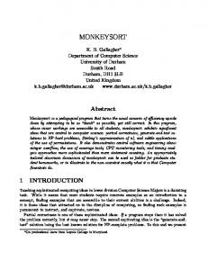
Example 31. For each a ∈ A, let σa = {(1, a)} and Pa = νb. p(ab)
′
p(ab) = a ¯b. νc. p(bc) .
In the π-calculus, Pa induces an infinitely-branching, infinite-path transition graph: 55 . 55 . 55 . lll .. lll .. ′ lll .. ′ ′ ¯ a ¯ (b ) lll b(c ) lll c ¯(d ) lll l l l llla¯(b) // lll c¯(d) // lll ¯b(c) // ··· Pc Pb Pa
In the extended calculus, Pa induces the following transition graph,
′ ¯′
π · a(b). b¯ c. 0 = a (b ). b c . 0 ′
with definition
1⊛
1
1
σa ⊢ Pa −→ σa ⊢ νb. b. νc. p(bc) −→ σb ⊢ Pb −→ · · ·
′
where a =π(a), b =π(b), c =π(c) (note that permutations equally affect bound and free name occurrences). Similarly to X ∗ , we have that X × Y is a nominal set whenever X and Y are. Note that if X is a nominal set and X ′ ⊆ X is such that π · x ∈ X ′ , for all x ∈ X ′ and π ∈ Perm(A), then X ′ is also a nominal set with the inherited action. Hence, the following set is a nominal set. [ ˆ ∧ fn(Pˆ ) ⊆ img(σ) } (1) ˆ = { (σ, Pˆ ) | σ ∈ Regn ∧ Pˆ ∈ Π K
which is economic by branching once at each step. In fact, setting Pout = νb. b. νc. p(bc), and since σa ⊢ Pa = σb ⊢ Pb and σa ⊢ Pout = σb ⊢ Pout for all a, b ∈ A, the graph above contains just two nodes: 1 (( σ ⊢ P σa ⊢ Pa hh a out 1⊛
and using double labels we get simply σa ⊢ PPa cc
n∈ω
11⊛
.
ˆ to elements (σ, Pˆ ) with Pˆ ∈ Π. We write K for the restriction of K Finally, from a nominal set X we can derive its set of orbits:
The way in which the two transition relations are related is given by the following lemma, which verifies the intuitions of Table 1.
O(X) = {O(x) | x ∈ X} where O(x) = {π·x | π ∈ Perm(A)}.
Lemma 32. Let σ, σ ′ be registers, and α, α ˆ be labels of π and xπ respectively. For all P, P ′ ∈ Π with fn(P ) ⊆ img(σ):
Note that each O(x) is a nominal subset of X. The technology of the previous paragraph is used for defining the transition system of the extended calculus. In contrast to the ordinary π-calculus, the transition relation we define is finitely branching, and this is achieved by considering processes-in-context and specifying channels by their context indices instead of their ˆ be the set of processes-innames. More specifically, we let O(K) ˆ context. Each such O(σ, P ) is written σ ⊢ Pˆ . Since σ ⊢ Pˆ = π·σ ⊢ π·Pˆ , for any permutation π, what matters in σ ⊢ Pˆ is not the specific names occurring in σ or P , but only their index in σ. For example,
α ˆ
α
There is a straightforward passage from the xπ-calculus to ˆ states from O(K) are final, FRA’s: states are taken from O(K), and the transition relation is the one given in Table 1 (omitting double transitions).7 However, the usual (symbolic) notion of bisimulation between FRA’s is not appropriate because it is defined for single-step transitions and, moreover, does not take into account the distinction between inputs and outputs. We therefore define the following notion. Definition 33. An n-simulation is a relation R ⊆ O(K) × ([n] ⇋ [n]) × O(K)
Definition 30. The semantics of the xπ-calculus is given via a ˆ and labels: labelled transition system with set of states O(K) α ::= i | i | i | τ | ¯ij | ¯ij
⊛
| ij | ij
′
where either α ˆ = α = τ and σ = σ ′ ; or α ˆ = ¯ij/ij, α = a ¯b/ab, σ(i) = a, σ(j) = b and σ ′ = σ; or α ˆ = ¯ij ⊛ /ij • , α = a ¯(b)/ab, σ(i) = a, σ ′ = σ[j 7→ b] and j = min{j | σ(j) ∈ / fn(P ′ )}.
and in essence both of these are specified by an expression e.g. like ({(1, ◦), (2, ◦)}, 1(b). b¯ 2. 0). Borrowing notation from FRA’s, we build up on the indices idea and use transition labels of the form i• /i⊛ for fresh inputs/outputs.
⊛
′
α ˆ
• if P −→ P then σ ⊢ P −→ σ ⊢ P ′ ;
{(1, a), (2, c)} ⊢ a(b). b¯ c. 0 = {(1, a′ ), (2, c′ )} ⊢ a′ (b). bc¯′ . 0
•
α
• if σ ⊢ P −→ σ ′ ⊢ P ′ then P −→ P ′ ,
6 Although
not essential, minimisation saves us from unnecessary branching. that this translation typically yields infinite FRA’s — but we shall examine classes of processes where the resulting FRA’s are finite in the end of this section.
•
7 Note
where i, j ∈ ω. The transition relation is given by the rules in Table1.
9
α
α
I NP 1
σ ⊢ P −→ σ ⊢ Pˆ′ α σ ⊢ [a = a]P −→ σ ⊢ Pˆ′
M ATCH
σ(i)=a
i
σ ⊢ a(b).P −→ σ ⊢ (b).P I NP 2 A
I NP 2 B
σ(i)=a
i
σ ⊢ (b).P −→ σ[i 7→ b] ⊢ P O UT 2
σ(i)=a
i
σ ⊢ b.P −→ σ ⊢ P
α (σ + a) ⊢ Pˆ −→ (σ ′ + a) ⊢ Pˆ ′ α σ ⊢ νa.Pˆ −→ σ ′ ⊢ νa.Pˆ ′
PAR 1
α σ ⊢ Pˆ −→ σ ⊢ Pˆ ′ α σ ⊢ Pˆ | Q −→ σ ⊢ Pˆ ′ | Q
¯ ij
C OMM
D BL O UT
p(~ b)=P
σ[i 7→ a] ⊢ Pout −→ σ[i 7→ a] ⊢ P
O PEN
i⊛
i=min{i | σ(i)∈fn(P / )}
σ ⊢ νa.Pout −→ σ[i 7→ a] ⊢ P •
⊛
i /i σ ⊢ Pˆ −→ σ[i 7→ b] ⊢ P ′
PAR 2
α= i/τ
j • /j ⊛
′ j=min{j | σ(j)∈fn(P / ,Q)}
σ ⊢ Pˆ | Q −→ σ[j 7→ b] ⊢ P ′ | Q
σ ⊢ Q −→ σ ⊢ Q′ τ
σ ⊢ P | Q −→ σ ⊢ P ′ | Q′
¯ i1⊛
C LOSE
j/j ⊛
i
α σ ⊢ P {~a/~b} −→ σ ⊢ Pˆ′ α σ ⊢ p(~a) −→ σ ⊢ Pˆ′
i
α6=(|σ|+1)
ij
σ ⊢ P −→ σ ⊢ P ′
R EC
σ(i)=b
i
σ⊢a ¯b.P −→ σ ⊢ b.P R ES
σ ⊢ P −→ σ ⊢ Pˆ ′ α σ ⊢ P +Q −→ σ ⊢ Pˆ ′
i=min{i | σ(i)∈fn(P / )}
i•
σ ⊢ (b).P −→ σ ⊢ P {a/b} O UT 1
S UM
(♯ + σ) ⊢ P −→ (b + σ) ⊢ P ′ τ
σ ⊢ P | Q −→ σ ⊢ νb.(P ′ | Q′ ) j/j •
i
σ ⊢ P −→ σ ⊢ Pout −→ σ ′ ⊢ P ′
D BL I NP
¯ ij/¯ ij ⊛
i1•
(♯ + σ) ⊢ Q −→ (b + σ) ⊢ Q′
σ ⊢ P −→ σ ⊢ Pinp −→ σ ′ ⊢ P ′ ij/ij •
σ ⊢ P −−−−→ σ ′ ⊢ P ′
σ ⊢ P −−−−→ σ ′ ⊢ P ′
Table 1. The transition relation for the xπ-calculus (symmetric counterparts of S UM , PAR , C OMM , C LOSE omitted8 ). such that if (σ1 ⊢ P1 , ρ, σ2 ⊢ P2 ) ∈ R then σ1 , σ2 ∈ Regn and
The set of reducts of a given process-in-context is in general infinite, even if the process is n-contained. The following result provides sufficient conditions for excluding such infinite behaviours. We say that a process has finite control if no parallel compositions appear in its recursive definitions. A process is ν-strict if all its subprocesses of the form νa.P satisfy a ∈ fn(P ).
α′
α
σ1 ⊢ P1 −→ σ1′ ⊢ P1′ implies that σ2 ⊢ P2 −→ σ2′ ⊢ P2′ for some (σ1′ ⊢ P1′ , ρ′ , σ2′ ⊢ P2′ ) ∈ R such that one of the following is the case, with i ∈ dom(ρ): • • • •
α = α′ = τ and ρ′ = ρ; α = ij, j ∈ dom(ρ), α′ = ρ(i)ρ(j) and ρ′ = ρ; α = ij, j ∈ / dom(ρ), α′ = ρ(i)k• and ρ′ = ρ[j ↔ k]; α = ij • , α′ = ρ(i)k• , ρ′ = ρ[j ↔ k] and,
Proposition 35. If P0 ∈ Π has finite control and all its descendants are ν-strict, then there are some M ∈ ω, σ0 ∈ RegM and a finite S ⊆ O(K) such that P0 is M -contained, (σ0 ⊢ P0 ) ∈ S and α for all (σ ⊢ P ) ∈ S if σ ⊢ P −→ σ ′ ⊢ P ′ then (σ ′ ⊢ P ′ ) ∈ S.
ρ(i)k′
for all k′ ∈ S2 (ρ) \ img(ρ), σ2 ⊢ P2 −→ σ2 ⊢ P2′ for some (σ1′ ⊢ P1′ , ρ[j ↔ k′ ], σ2 ⊢ P2′ ) ∈ R; • α = ¯ij, j ∈ dom(ρ), α′ = ρ(i)ρ(j) and ρ′ = ρ; • α = ¯ij ⊛ , α′ = ρ(i)k ⊛ and ρ′ = ρ[j ↔ k].
Proof. Suppose (WLOG) that P0 invokes definitions pi (~ai ) = Pi , i ∈ [N ] for some N , and take M = |P0 | × max{ |Pi | | i ∈ [N ] } for the size function which counts a process’ occurrences of 0’s, p’s and names, free or bound (but not binding): e.g. |¯ ab.P | = 2 + |P |, |a(b).P | = 1 + |P |, |νa.P | = |P |, |p(~a)| = 1 + |~a| and |0| = 1. If Q is a descendant of P then |Q| ≤ M as a process may only increase its size by recursion and, as P0 has finite control, recursions cannot obtain size greater than max{ |Pi | | i ∈ [N ] }. But then, because all descendants of P0 are ν-strict, their number of ν-abstractions is bounded by M , and hence they all have length (number of symbols or constructors) bounded relatively to M . They are still unboundedly many, due to different choices of free variables. But since each descendant can be matched with a context from RegM , the number of the resulting processes-in-context is bounded relatively to M . We collect all these in S.
R is called an n-bisimulation if both R and R−1 are n-simulations. n P1 and P2 are n-bisimilar, written P1 ∼ P2 , if there is an nbisimulation R containing (σ01 ⊢ P1 , σ01 ↔ σ02 , σ02 ⊢ P2 ), for some σ01 , σ02 with img(σ01 ) = fn(P1 ), img(σ02 ) = fn(P2 ). We say that a process is n-contained if all its descendants have less than n free names. π
n
Proposition 34. For all n-contained P, Q, P ∼ Q iff P ∼ Q. Proof. The proof proceeds by showing that if R is a simulation for the π-calculus then R′ = { (σ1 ⊢ P1 , ρ, σ2 ⊢ P2 ) | (P1 , P2 ) ∈ R ∧ ρ = σ1 ↔ σ2 }
Corollary 36. Bisimilarity is decidable in Π when restricted to processes with finite control.
with P1 , P2 n-contained and σ1 , σ2 ∈ Regn is an n-simulation and, conversely, if R is an n-simulation then R′ = { (P1 , P2 ) | ∃σ1 , σ2 . (σ1 ⊢ P1 , σ1 ↔ σ2 , σ2 ⊢ P2 ) ∈ R } with P1 , P2 n-contained is a simulation for π. 8 note: σ+v
= σ∪{(|σ|+1, v)}, v+σ = {(1, v)}∪{(i+1, v′ ) | (i, v′ ) ∈ σ}.
10
Proof. For any such processes P1 , P2 ∈ Π, by the previous proposition and after equating processes up to non-strict ν-abstractions, we obtain M -transition graphs with sizes bounded relatively to P1 M and P2 . Clearly, P1 ∼ P2 iff there is an M -bisimulation between
A. Proofs from section 6
those graphs. As those bisimulations live in a space bounded relatively to the sizes of P1 and P2 , we can search it exhaustively for such relations.
Proof of Lemma 19. Let A = hQ, q0 , σ0 , δ, F i. The construction of B = hQ′ , q0′ , σ0′ , δ ′ , F ′ i follows closely [11]. In particular, each transition of A involving a name induces an assignment of that name in the extra register of B. If the transition were a fresh assignment then this would result in the name occurring in B just once after assignment, otherwise it would occur twice. As the actual extra register of B changes during this process we add an extra component in states to remember it. ∼ = We set Q′ = Q × ([n + 1] − → [n + 1]) and write elements of ′ ′ Q as (q, π). Moreover, q0 = (q0 , id), σ0′ = σ0 [n+1 7→ ♯] and F ′ = {(q, π) | q ∈ F }. Finally:
Equating processes up to structural congruence [14], the above results can be further strengthened to processes with finite degree of parallelism, in a similar manner to [4].
9. Further directions We have introduced an abstract computational paradigm and established its key properties, laying the ground for further research. The next logical step is to examine concrete applications of FRA’s to the description of computation with names, either in the direction of mobile calculi or that of programming languages, relating this approach to existing higher-level approaches. A first such advance has been recently accomplished in [19] by constructing a model of a low-order restriction of Reduced ML (a fragment of ML with ground-type integer references) representable in a variant of FRA’s where labels contain store information. This was achieved by representing the fully abstract game semantics of the language [18]. On the foundational side, the study of the π-calculus in FRA’s revealed that there is a notion of polarity inherent in computation with names. In particular, the examined FRA’s do not mix locally with globally fresh transitions, and this is clearly depicted in the ˆ = Πinp ⊎ Πout ⊎ Π. A similar observation applies to partition Π FRA’s describing Reduced ML [19]. There, the states are partitioned in P-states (for Proponent/Program) and O-states (for Opponent/Environment); only P-states are allowed to perform globally fresh transitions, and only O-states can do locally fresh ones. Intuitively, the only notion of freshness that can be observed on the program’s side is local freshness, whereas the environment should be assumed to have the memory needed in order to observe global freshness. These observations suggest that a notion of polarised FRA, where states are partitioned as above, is relevant and should be further pursued. In the polarised setting, symbolic bisimulations are simplified as there is no longer need for an h component (cf. Definitions 25 and 33). A potential criticism towards FRA’s concerns the fact that they fail to satisfy closure under concatenation and Kleene star (cf. Section 6). We find these non-closure results rather expected as FRA’s are history-sensitive machines. On the other hand, FRA’s seem to be closed under the nominal versions of concatenation and Kleene star, as recently introduced by Gabbay and Ciancia [9]. The precise connections between FRA’s and regular languages with namerestriction [9] are the subject of ongoing research. Finally, some important questions have still not been answered. For example, we have not considered deterministic versions of FRA’s, nor examined whether FRA’s can be determinised. Assuming that in a deterministic FRA to each input string corresponds a unique path, we can see that e.g. the FRA accepting the language
δ ′ = { ((q1 , π), ℓ, (q2 , π)) | ℓ ∈ C ∧ (q1 , ℓ, q2 ) ∈ δ } ∪ { (q1′ , ({π(n+1)}, {π(i), π(n+1)}), (q2 , π)) | (q1 , i, q2 ) ∈ δ } ∪ { (q1′ , ({π(n+1)}, {π(n+1)}), (q2 , π ′ )) | (q1 , i• , q2 ) ∈ δ } ∪ { (q1′ , ({π(n+1)}, {π(n+1)}, [n]), (q2 , π ′ )) | (q1 , i⊛ , q2 ) ∈ δ } where q1′ = (q1 , π) and π ′ = (π(i) ↔ π(n+1)) ◦ π (we write (k ↔ j) for the permutation that swaps k and j). We can show that the following relation is a bisimulation and therefore that A ∼ B. R = { ((q, σ, H), ((q, π), σ ′ , H)) | ∀i ∈ [n]. σ(i) = σ ′ (π(i)) } Proof of Lemma 20. Let A = hQ, q0 , σ0 , δ, F i and construct B = hQ′ , q0′ , σ0′ , δ ′ , F ′ i as follows. The idea is to keep in the extra memory registers of B a copy of the initial configuration σ0 which is never touched by assignments. Thus, whenever A wants to make a transition with label (S, T, A), B will simulate it by a transition (S, S, [n]) and transitions of the form (S, T ∪ Ta ) where Ta ⊆ {n+1, ..., 2n}, a ∈ σ0 ([n] \ A) and a is not in the history. In order to accomplish this we need to enrich states with information regarding whether the names in img(σ0 ) appear in the history. Therefore, we set Q′ = Q × P(img(σ0 )), q0′ = (q0 , ∅), σ0′ = σ0 + σ0 , F ′ = {(q, I) | q ∈ F } and: δ ′ = { ((q, I), ℓ, (q ′ , I)) | ℓ ∈ C ∧ (q, ℓ, q ′ ) ∈ δ } ∪ { ((q, I), (S, T ), (q ′ , I)) | (q, (S, T ), q ′ ) ∈ δ } ∪ { ((q, I), (S, T ∪ Ta ), (q ′ , I ∪ {a})) | (q, (S, T ), q ′ ) ∈ δ } ∪ { ((q, I), (S, S, [n]), (q ′ , I)) | (q, (S, S, A), q ′ ) ∈ δ } ∪ { ((q, I), (S, T ∪ Ta′ ), (q ′ , I ∪ {a′ })) | (q, (S, T, A), q ′ ) ∈ δ } where a ∈ img(σ0 ), Ta = { (n + i) ∈ [2n] | σ0 (i) = a }, a′ ∈ σ0 ([n] \ A) \ I, and Ta′ as Ta . We can check that R = { ((q, σ, H), ((q, I), σ ′ , H)) | I = H∩img(σ0 )∧σ ′ = σ+σ0 } is a bisimulation and therefore that A ∼ B. Proof of Lemma 21. Let A = hQ, q0 , σ0 , δ, F i and construct B = hQ′ , q0′ , σ0′ , δ ′ , F ′ i by setting Q′ = Q × ([n] → [n]) and selecting f0 , σ0′ such that img(σ0 ) = img(σ0′ ) and σ0 = σ0′ ◦ f0 . Moreover, set q0′ = (q0 , f0 ), F ′ = {(q, f ) | q ∈ F } and:
L = { a1 · · · ak a | a ∈ {a1 , . . . , ak } ∧ ∀i 6= j. ai 6= aj } has no deterministic equivalent. Other directions for further research concern minimisation of FRA’s (recently examined for FMA’s [2]) and the evident connections to HD-automata. Moreover, several possible extensions of FRA’s are of interest, e.g. variants with labels (data words), stores, or pushdown variants.
δ ′ = { ((q, f ), ℓ, (q ′ , f )) | ℓ ∈ C ∧ (q, ℓ, q ′ ) ∈ δ } ∪ { ((q, f ), i, (q ′ , f ′ )) | f (T \ S) = {i} ∧ (q, (S, T ), q ′ ) ∈ δ } ∪ { ((q, f ), i, (q ′ , f ′ )) | f −1 (i) ⊆ S ∧ (q, (S, S), q ′ ) ∈ δ } ∪ { ((q, f ), i• , (q ′ , f ′ )) | f −1 (i) ⊆ S ∧ (q, (S, S), q ′ ) ∈ δ } ∪ { ((q, f ), i⊛ , (q ′ , f ′ )) | f −1 (i) ⊆ S ∧ (q, (S, S, [n]), q ′ ) ∈ δ }
10. Acknowledgements
with f ′ = f [S 7→ i]. Now, the following is a bisimulation
Thanks to Andrzej Murawski, Samson Abramsky, Vassilis Koutavas and Ulrich Sch¨opp for discussions and suggestions. Thanks also to the anonymous reviewers for their comments. Section 7 in particular is now much simpler due to a reviewer’s suggestion.
R = { ((q, σ, H), ((q, f ), σ ′ , H)) | σ = σ ′ ◦ f } and hence A ∼ B.
11
B. Proofs from section 7
References
Proof of Proposition 26. It will suffice to check only non-constant transitions. So let ((q1 , σ1 , H), (q2 , σ2 , H)) ∈ R′ due to some a (q1 , h, ρ, q2 ) ∈ R and suppose that (q1 , σ1 , H) −→δ1 (q1′ , σ1′ , H ′ ) ′ with H = H ∪ {a}. We do case analysis on a. Below we write ρ′ for ρ[i ↔ j]. • a ∈ img(σ1 ) ∩ img(σ2 ), say a = σ1 (i) = σ2 (j). Then, it is necessary that (q1 , i, q1′ ) ∈ δ1 and σ1′ = σ1 . Also, ρ = σ1 ↔ σ2 implies (i, j) ∈ ρ, so (q2 , j, q2′ ) ∈ δ2 for some (q1′ , h, ρ, q2′ ) ∈ R. a ˆ′ = H ˆ so Thus, (q2 , σ2 , H) −→δ2 (q2′ , σ2 , H ′ ) and, noting that H ˆ ′ |⌉n , we can see that ((q1′ , σ1 , H ′ ), (q2′ , σ2 , H ′ )) ∈ R′ . h = ⌈|H • a ∈ img(σ1 )\img(σ2 ), say a = σ1 (i). Then, again (q1 , i, q1′ ) ∈ δ1 and σ1′ = σ1 , but i ∈ S1 (ρ) \ dom(ρ). Thus, (q2 , j • , q2′ ) ∈ δ2 a for some (q1′ , h, ρ′ , q2′ ) ∈ R. Thus, (q2 , σ2 , H) −→δ2 (q2′ , σ2′ , H ′ ), ′ ′ ′ ˆ ′ = H, ˆ we have σ2 = σ2 [j 7→ a]. Noting that ρ = σ1 ↔ σ2 and H ′ ′ ′ ′ ′ ′ that ((q1 , σ1 , H ), (q2 , σ2 , H )) ∈ R . ˆ \ img(σ1 ), • a ∈ img(σ2 ) \ img(σ1 ), say a = σ2 (j). Since a ∈ H we have some (q1 , i• , q1′ ) ∈ δ1 , and σ1′ = σ1 [i 7→ a]. Moreover, j ∈ S2 (ρ) \ img(ρ) and therefore (q2 , j, q2′ ∈ δ2 for some a (q1′ , h, ρ′ , q2′ ) ∈ R. Thus, (q2 , σ2 , H) −→δ2 (q2′ , σ2 , H ′ ) and we ′ ′ ′ ′ ′ can see that ((q1 , σ1 , H ), (q2 , σ2 , H )) ∈ R′ . ˆ \ (img(σ2 ) ∪ img(σ1 )), so (q1 , i• , q1′ ) ∈ δ1 , and σ1′ = • a∈H ˆ = h. σ1 [i 7→ a]. If h < n then kρk = |img(σ1 ) ∪ img(σ2 )| < |H| Thus, (q2 , j • , q2 ) ∈ δ2 for some (q1′ , h, ρ′ , q2′ ) ∈ R, and so a (q2 , σ2 , H) −→δ2 (q2′ , σ2′ , H ′ ), σ2′ = σ2 [j 7→ a]. We have ρ′ = ˆ ′ |⌉n , thus ((q1′ , σ1′ , H ′ ), (q2′ , σ2′ , H ′ )) ∈ R′ . σ1′ ↔ σ2′ and h = ⌈|H ˆ and say transition is due to (q1 , i• /i⊛ , q1′ ) ∈ δ1 , so σ1′ = • a∈ /H σ1 [i 7→ a]. Then, (q2 , j • /j ⊛ , q2′ ) ∈ δ2 for some (q1′ , h++ , ρ′ , q2′ ) ∈ a R, so (q2 , σ2 , H) −→δ2 (q2′ , σ2′ , H ′ ), σ2′ = σ2 [j 7→ a]. We have ˆ ′ |⌉n , so ((q1′ , σ1′ , H ′ ), (q2′ , σ2′ , H ′ )) ∈ R′ . that h++ = ⌈|H Thus, R′ is a simulation. If R is a symbolic bisimulation then, by symmetry, R′ is a bisimulation. Finally, if (q01 , |H0 |, σ01 ↔ σ02 , q02 ) ∈ R then ((q01 , σ01 , ∅), (q02 , σ02 , ∅)) ∈ R′ .
[1] S. Abramsky, D. R. Ghica, A. S. Murawski, C.-H. L. Ong, and I. D. B. Stark. Nominal games and full abstraction for the nu-calculus. In Proc. of LICS ’04, pages 150–159. IEEE Comp. Soc. Press, 2004. [2] M. Benedikt, C. Ley, and G. Puppis. Minimal memory automata. Alberto Mendelzon Workshop on Foundations of Databases, 2010. [3] N. Benton and V. Koutavas. A mechanized bisimulation for the nucalculus. Tech. Rep. MSR-TR-2008-129, Microsoft Research, 2008. [4] R. Bruni, F. Honsell, M. Lenisa, and M. Miculan. Modeling fresh names in the pi-calculus using abstractions. In Proc. of CMCS ’04, volume 106, pages 25–41. Elsevier, 2004. [5] S. Delaune, S. Kremer, and M. Ryan. Symbolic bisimulation for the Applied Pi Calculus. In Proc. of FSTTCS ’07, volume 4855 of LNCS, pages 133–145, 2007. [6] S. Demri and R. Lazic. LTL with the freeze quantifier and register automata. ACM Trans. Comput. Log., 10(3), 2009. [7] G. L. Ferrari, U. Montanari, and E. Tuosto. Model checking for nominal calculi. In Proc. of FOSSACS ’05, volume 3441 of LNCS, pages 1–24, 2005. [8] M. Gabbay and A. M. Pitts. A new approach to abstract syntax with variable binding. Formal Asp. Comput., 13(3-5):341–363, 2002. [9] M. J. Gabbay and V. Ciancia. Freshness and name-restriction in sets of traces with names. Submitted for publication, 2010. [10] A. Jeffrey and J. Rathke. Towards a theory of bisimulation for local names. In LICS, pages 56–66, 1999. [11] M. Kaminski and N. Francez. Finite-memory automata. Theor. Comput. Sci., 134(2):329–363, 1994. [12] J. Laird. A game semantics of local names and good variables. In Proc. of FOSSACS ’04, volume 2987 of LNCS, pages 289–303, 2004. [13] J. Laird. A fully abstract trace semantics for general references. In Proc. of ICALP ’07, volume 4596 of LNCS, pages 667–679, 2007. [14] R. Milner, J. Parrow, and D. Walker. A calculus of mobile processes, I and II. Inf. Comput., 100(1):1–77, 1992. [15] R. Milner, M. Tofte, and D. Macqueen. The Definition of Standard ML. MIT Press, 1997. [16] U. Montanari and M. Pistore. An introduction to History Dependent Automata. Electr. Notes Theor. Comput. Sci., 10, 1997. [17] U. Montanari and M. Pistore. Structured coalgebras and minimal HDautomata for the pi-calculus. Theor. Comput. Sci., 340(3):539–576, 2005. [18] A. S. Murawski and N. Tzevelekos. Full abstraction for Reduced ML. In Proc. of FOSSACS ’09, volume 5504 of LNCS, pages 32–47, 2009. [19] A. S. Murawski and N. Tzevelekos. Algorithmic nominal game semantics. Submitted for publication, 2010. [20] R. M. Needham. Names. In S. Mullender, editor, Distributed systems, pages 315–327. ACM Press/Addison-Wesley, 1993. 2nd edition. [21] F. Neven, T. Schwentick, and V. Vianu. Finite state machines for strings over infinite alphabets. ACM Trans. Comput. Logic, 5(3):403– 435, 2004. [22] M. Pistore. History Dependent Automata. PhD thesis, University of Pisa, 1999. [23] A. M. Pitts. Nominal logic, a first order theory of names and binding. Inf. Comput., 186(2):165–193, 2003. [24] A. M. Pitts and I. Stark. Observable properties of higher order functions that dynamically create local names, or: What’s new? In Proc. of MFCS ’93, number 711 in LNCS, pages 122–141, 1993. [25] H. Sakamoto and D. Ikeda. Intractability of decision problems for finite-memory automata. Theor. Comput. Sci., 231(2):297–308, 2000. [26] D. Sangiorgi and D. Walker. The pi-calculus: A Theory of Mobile Processes. Cambridge University Press, 2001. [27] L. Segoufin. Automata and logics for words and trees over an infinite alphabet. In Proc. of CSL ’06, vol. 4207 of LNCS, pages 41–57, 2006. [28] I. Stark. Names and Higher-Order Functions. PhD thesis, University of Cambridge, 1994.
Proof of Proposition 27. We check non-constant transitions. Let (q1 , h, ρ, q2 ) ∈ R′ , due to some ((q1 , σ1 , H), (q2 , σ2 , H)) ∈ R and suppose that (q1 , ℓ, q1′ ) ∈ δ1 . We do case analysis on ℓ. Below we write H ′ for H ∪ {a}, and ρ′ for ρ[i ↔ j]. a • If ℓ = i then, by closure, (q1 , σ1 , H) −→δ1 (q1′ , σ1 , H ′ ) with a a = σ1 (i), and hence (q2 , σ2 , H) −→δ2 (q2′ , σ2′ , H ′ ) for some ((q1′ , σ1 , H ′ ), (q2′ , σ2′ , H ′ )) ∈ R. If i ∈ dom(ρ), say (i, j) ∈ ρ, then a ∈ img(σ2 ) and it must be (q2 , j, q2′ ) ∈ δ2 , σ2′ = σ2 . We can see that (q1′ , h, ρ, q2′ ) ∈ R′ . If i ∈ S1 (ρ) \ dom(ρ) then a ∈ / img(σ2 ) and there is some (q2 , j • , q2′ ) ∈ δ2 , and ′ σ2 = σ2 [j 7→ a]. We have that (q1′ , h, ρ′ , q2′ ) ∈ R′ . a • If ℓ = i• then, for each a ∈ / img(σ1 ), (q1 , σ1 , H) −→δ1 a (q1′ , σ1′ , H ′ ), σ1′ = σ1 [i 7→ a], and therefore (q2 , σ2 , H) −→δ2 ′ ′ ′ ′ ′ ′ ′ ′ ′ (q2 , σ2 , H ) for some ((q1 , σ1 , H ), (q2 , σ2 , H )) ∈ R. For any j ∈ S2 (ρ) \ img(ρ), σ2 (j) ∈ / img(σ1 ), so we can take a = σ2 (j). Then, we must have (q2 , j, q2′ ) ∈ δ2 , σ2′ = σ2 , and we can check that (q1′ , h, ρ′ , q2′ ) ∈ R′ . ˆ \ (img(σ1 ) ∪ If h = n or kρk < h then we can choose a ∈ H img(σ2 )). Thus, we have some (q2 , j • , q2′ ) ∈ δ2 , σ2′ = σ2 [j 7→ a]. ˆ′ = H ˆ and ρ′ = σ1′ ↔σ2′ , we get (q1′ , h, ρ′ , q2′ ) ∈ R′ . Noting that H ˆ then there is some (q2 , j • /j ⊛ , q2′ ) ∈ Finally, if we choose a ∈ / H δ2 , and σ2′ = σ2 [j 7→ a]. We have that ρ′ = σ1′ ↔ σ2′ and ˆ′ = H ˆ ⊎{a}, thus h++ = ⌈|H ˆ ′ |⌉n . Hence, (q1′ , h++ , ρ′ , q2′ ) ∈ R′ . H • If ℓ = i⊛ then we work as in the last case above. Thus, R′ is a symbolic simulation. If R is a bisimulation then, by symmetry, R′ is a symbolic bisimulation. Finally, if ((q01 , σ01 , ∅), (q02 , σ02 , ∅)) ∈ R then (q01 , |H0 |, σ01 ↔ σ02 , q02 ) ∈ R′ .
12